HTML
--> --> -->These methods allow us to estimate the prediction time within which weather forecasts are credible. However, the general public and policymakers are often more concerned with the prediction lead time of specific weather events such as extreme heat waves or heavy rainfall that can cause socioeconomic damage. The predictability of extreme weather events is different from that of normal weather events. To distinguish the predictability of specific weather events from that of normal weather events, Li et al. (2019) proposed two new notions of predictability: the local forward and local backward predictabilities. The local forward predictability is associated with the prediction time of normal weather events, while the local backward predictability is concerned with the maximum prediction lead time of extreme weather events. In current operational forecasts, owing to some uncertainties present in the observations and models, forecasts in the first few days are sufficiently accurate to inform the public well. Questions arise as to whether the accurate forecast time can be extended, and how to determine the upper predictability limit from initial normal events, but these questions are unsolved. Though two weeks are widely recognized as the upper limit, this problem still needs more intensive examination. In order to address this problem, Li et al. (2019) introduced the notion of local forward predictability to study the upper predictability limit from initial normal states. Since extreme weather events occur at a low frequency, their predictabilities are unique and differ from those of normal weather events (Mu et al., 2002; Chou, 2011). It is more difficult to estimate the predictability of extreme weather events. In order to estimate the predictability of extreme weather events, Li et al. (2019) indicated that the growing forecast errors resulting in such events should be analyzed, and proposed the notion of local backward predictability to study these kinds of events. Hence, the forward and backward predictabilities are focused on different kinds of weather events. Li et al. (2020b) studied the relative roles of initial condition and model errors in local forward predictability in the Lorenz model and found that the initial condition errors are more dominant in the forward predictability than model errors, consistent with previous studies (e.g. Downton and Bell, 1988; Lorenz, 1989; Richardson, 1998). The complexity of the predictability of specific weather events has meant that there are very few relevant studies on the relative roles of the two types of errors in local backward predictability. The occurrence of specific states, especially extreme states, has a greater impact on human society, so it is necessary to study the relative effects of the two types of errors on the local backward predictability of specific states, which may provide theoretical guidance for improving forecast skill. Ding and Li (2007) introduced the NLLE method to quantify the maximum prediction time from a random initial state. However, this technique can’t quantify how much time a specific state can be predicted in advance. In order to address this problem, Li et al. (2019) developed the backward nonlinear local Lyapunov exponent (BNLLE) method on the basis of the NLLE technique. By calculating the time of forecast errors growing to saturation level from the corresponding initial state to the specific state, the local predictability of the specific state can be quantified. Therefore, the NLLE and BNLLE techniques have different research objects. The NLLE method has been widely used in the atmospheric predictability or related fields (e.g., Li and Ding, 2013; He et al., 2021). However, since the BNLLE method was introduced, it has just been applied to a single study comparing the predictabilities of warm and cold events (Li et al., 2020a). In the present work, we will perform a theoretical study to investigate the relative effects of initial condition and model errors on the local backward predictability of specific states based on the BNLLE method. The BNLLE method is used to quantify the local backward predictability limit (LBPL) of a specific state. Therefore, the relative effects of initial condition and model errors on local backward predictability can be quantitatively estimated by comparing the difference between the LBPLs. The remainder of this paper is organized as follows. Section 2 introduces the BNLLE method and Lorenz model. The results of quantitative comparisons of the relative effects of initial condition and model errors on local backward predictability are presented in section 3. Finally, a discussion and conclusions are given in section 4.
2.1. Model description
In this work, the Lorenz model (1963, hereafter referred to as Lorenz63 model) is used to investigate the relative impacts of two types of uncertainties on local backward predictability. The Lorenz63 model is a conceptual model of the real atmosphere and has been widely used in studies of atmospheric predictability (e.g. Palmer, 1993; Evans et al., 2004; He et al., 2006, 2008; Feng et al., 2014; Li et al., 2020a). The detailed description of model setup parallels that of Li et al. (2020b).2
2.2. BNLLE method
Ding and Li (2007) proposed the NLLE method to quantitatively estimate atmospheric predictability. Figure 1 shows the mean local relative error growth of initial errors as a function of time for different error magnitudes in the Lorenz63 model. The initial errors grow with a regularly oscillating pattern at the early stage. After that, the errors reach a saturation level and cease to grow. For different magnitudes of initial error, the time to reach saturation is different. Smaller initial errors take more time to reach saturation. Before the saturation stage, the errors grow in the linear regime. When the errors are in the period of saturation, the nonlinearity dominates the error growth (e.g. Lacarra and Talagrand, 1988; Farrell, 1990; Lorenz, 2005). Therefore, the local forward predictability limit of a single state in phase space can be measured as the time when the forecast error exceeds 95% of the saturation value (Li et al., 2019).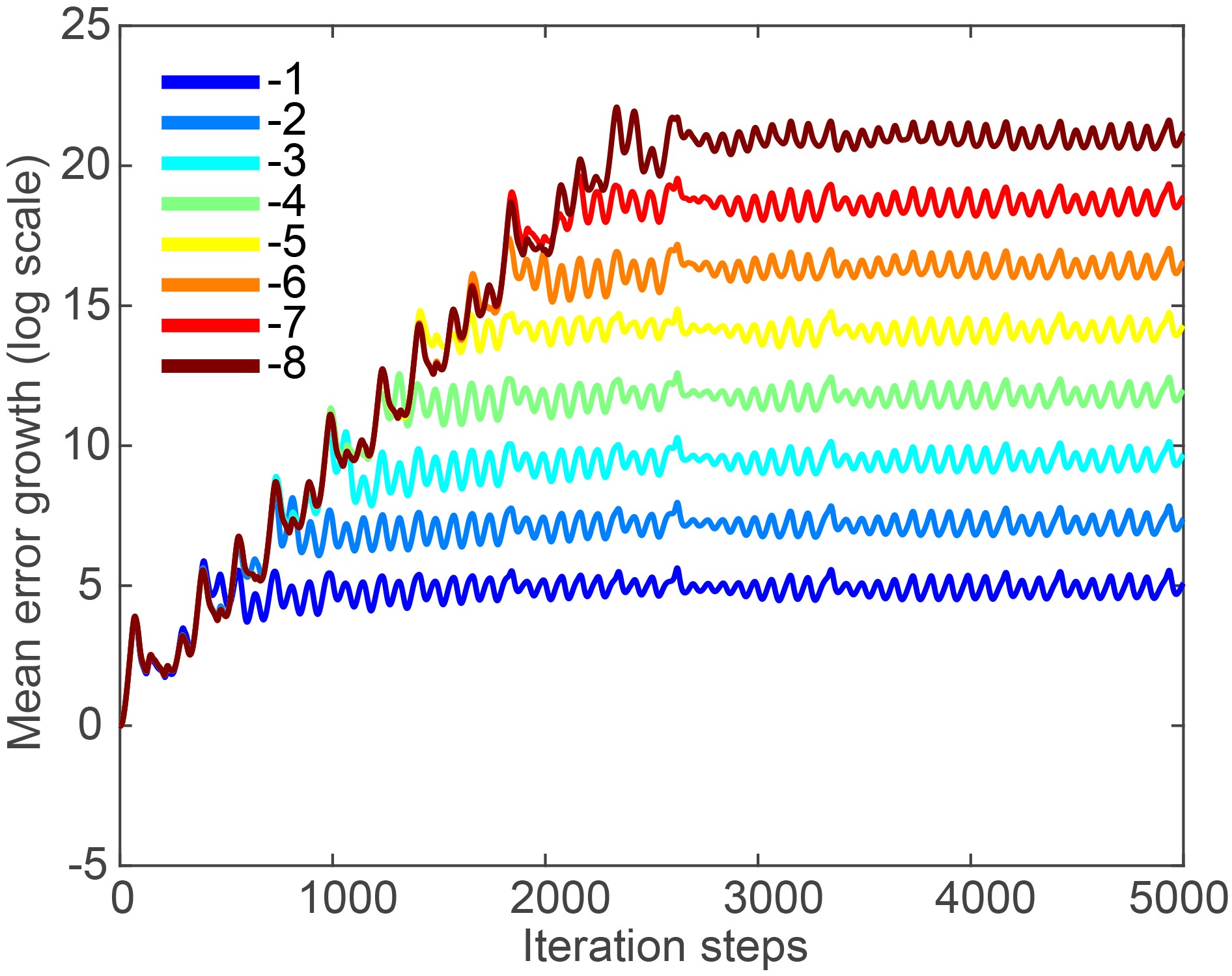 Figure1. Mean growth of initial errors with different magnitudes (log10 scale), for magnitudes of 10–1, 10–2, 10–3, 10–4, 10–5, 10–6, 10–7, and 10–8. The mean error growths are given in terms of natural logarithms (base e).
Using the NLLE algorithm, we can obtain the local forward predictability limit of any initial state. However, we cannot estimate the LBPL of a given state, especially for the extreme states that are of greater interest. On the basis of the NLLE algorithm, Li et al. (2019) introduced an algorithm, BNLLE, for estimating the LBPL of a given state. In an n-dimensional system, the growth of small errors


where


where


Figure 2 shows the simple procedure for determining the LBPL of the given state


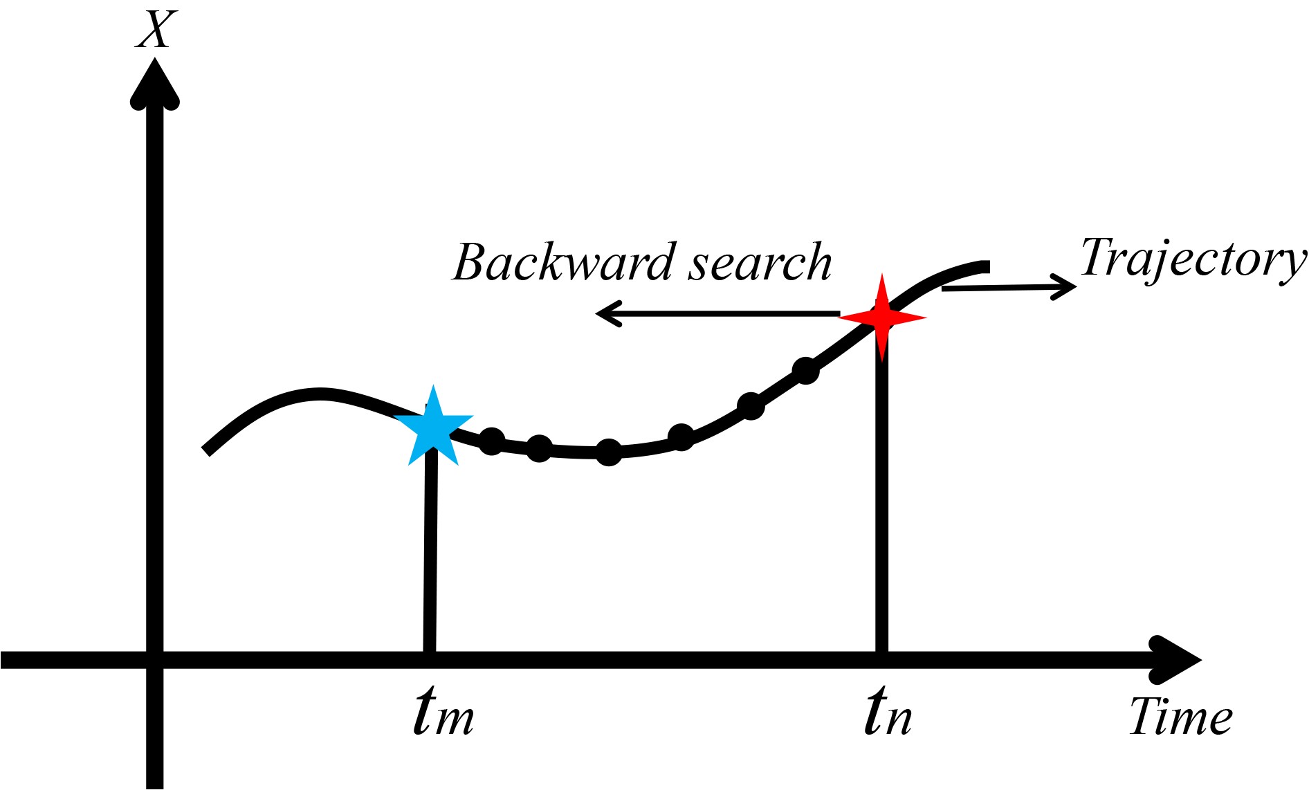 Figure2. Schematic of the algorithm used to estimate the LBPL of given state

3.1. Scenario one: Only initial condition errors
To investigate the effects of initial condition errors on the local backward predictability of given states, the model should be perfect. If (


Here


Figure 3 shows the spatial distribution of the LBPLs of these consecutive states. The figure shows two unstable stationary points, (


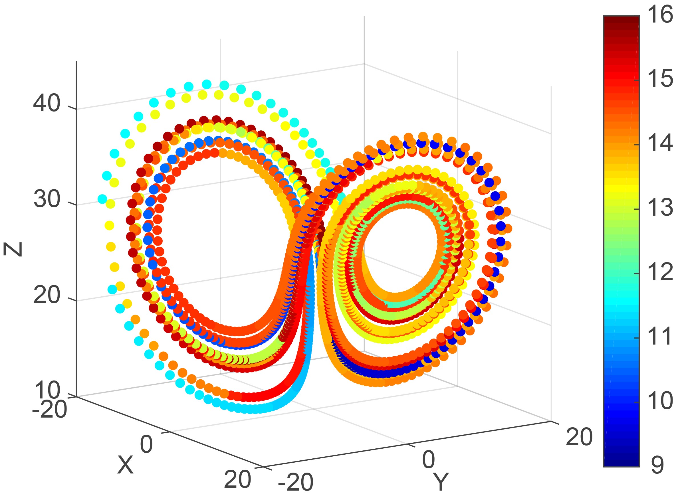 Figure3. Spatial distribution of LBPLs for 2,000 consecutive initial conditions from the given state (?0.46, 5.02, 30.90) on the Lorenz attractor
We also investigated the effects of the magnitude of initial condition errors on the LBPLs of given states. In order to make the conclusion more robust, the selected states should have different dynamical properties. We selected two states [(?0.61, 2.66, 28.49) and (–3.87, –5.69, 18.00)], the former of which is located in the dynamically unstable region, while the latter is located in the cold regime. Thus, they represent different dynamical flows and have different dynamical properties. The LBPLs of the two given states (Fig. 4) reveal that the LBPLs decrease as the size of the initial condition errors increases. For different given states, initial condition errors of the same size have different influences. When the magnitude of the initial condition errors is 10?7, the LBPLs of (?0.61, 2.66, 28.49) is 15 time units, while that of (?3.87, ?5.69, 18.00) is 19 time units. For other error magnitudes, the LBPLs are also different. This is because the local backward predictabilities depend on the given state on the dynamical trajectory. The two given states are on different locations of the dynamical flows, and the predictability varies with location; consequently, the LBPLs of the two given states are different, although the magnitudes of the initial condition errors superposed on them are the same.
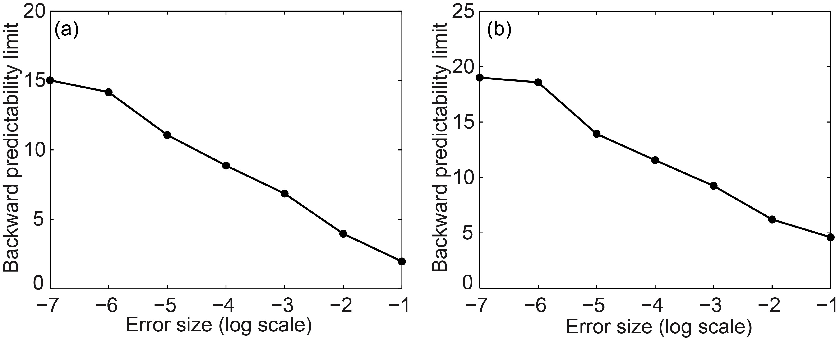 Figure4. Variation of LBPLs for initial condition errors for given states (a) (?0.61, 2.66, 28.49) and (b) (–3.87, –5.69, 18.00). Error size is shown on a log10 scale.
2
3.2. Scenario two: Only model errors
For the scenario of model errors without initial errors, the model is imperfect. Likewise, we perturbed three parameters with small perturbations in the Lorenz63 model.Here


Figure 5 shows the spatial distribution of LBPLs of the 2000 consecutive states; the LBPLs induced by model errors also show layered structures similar to those induced by initial condition errors. It is the specific structure of the Lorenz attractor determines the specific spatial distributions of the LBPLs. Therefore, the above results indicate that structure of the attractor has greater effects on predictability limits and their distributions. We also investigate the effects of model error magnitude on the LBPLs of given states. The situation is the same as for initial condition errors (shown in Fig. 6). Increasing the model error magnitude reduces the LBPLs of given states. The LBPLs of different given states are different, although the model error magnitudes are the same.
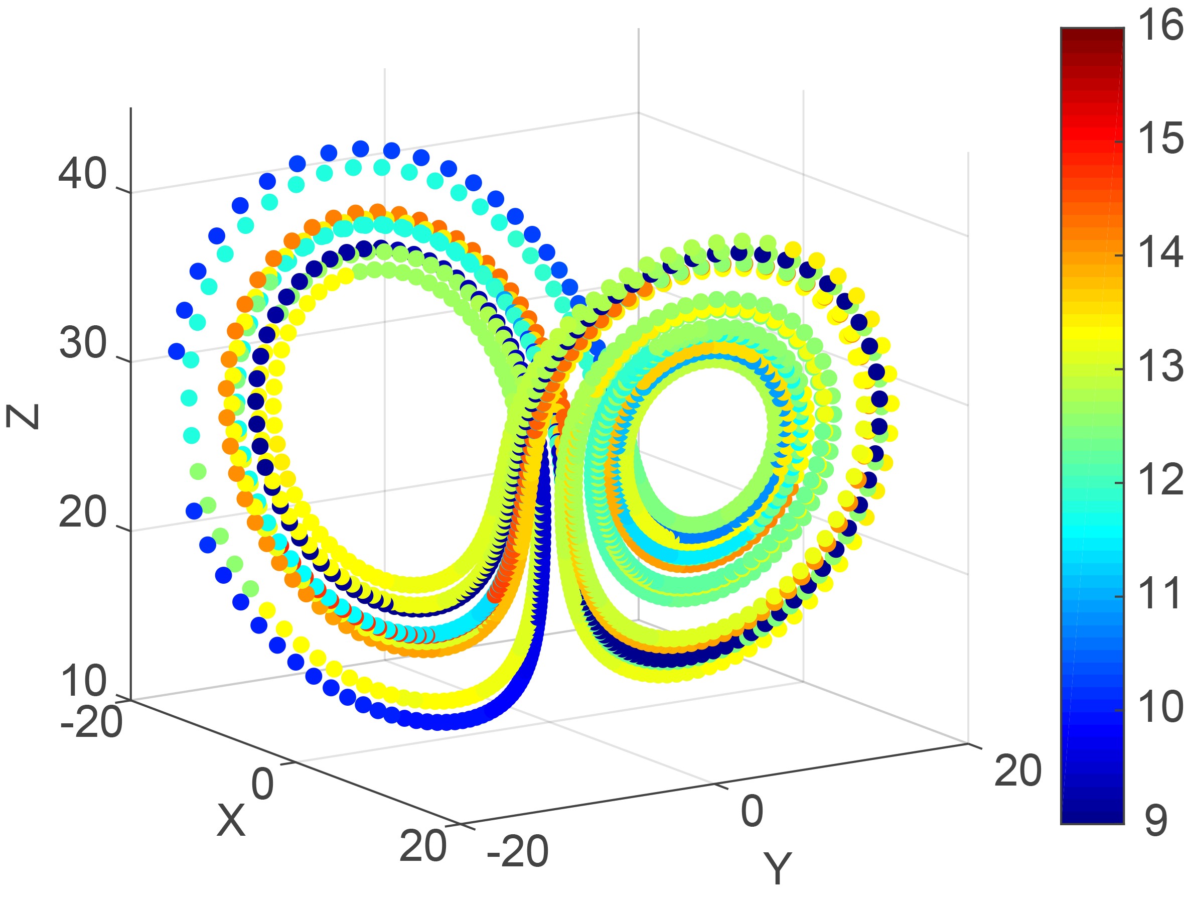 Figure5. Same as Fig. 3, but for the model error.
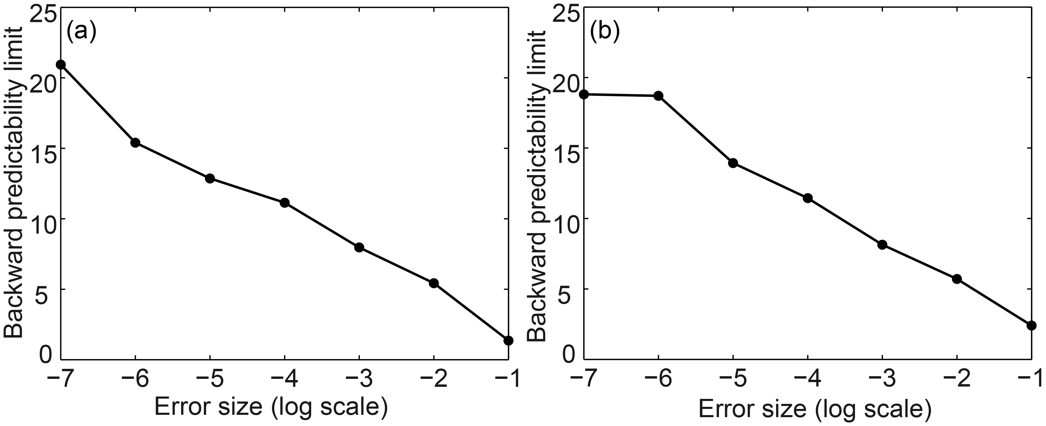 Figure6. Same as Fig. 4, but for the model error.
2
3.3. Relative effects of initial condition and model errors
The existence of initial condition and model errors affects the predictability, which leads to an upper limit. To quantify the relative effects of initial condition and model errors on the local backward predictability of given states, we compare the LBPLs they induce. In the case when the LBPLs of the given state induced by initial condition errors are higher than those of the same given state induced by model errors, this indicates that model errors have a larger impact, resulting in a lower local predictability limit, and vice versa. Figure 7 shows the variation of the LBPLs of two given states with the magnitude of the two types of errors. In Fig. 7a, for the given state (?0.54, 1.88, 26.43) and an error magnitude of 10–7, the LBPLs induced by model errors are slightly higher than those induced by initial condition errors. This demonstrates that initial condition errors have a greater influence on LBPLs, resulting in lower predictability. When the error magnitude is 10–2, the LBPLs induced by the two types of errors are roughly the same, so the initial condition and model errors have the same effects on local backward predictability. For other error magnitudes, the LBPLs induced by model errors are lower, indicating model errors have more influence. Therefore, when error magnitudes are different, the relative roles of initial condition and model errors in LBPLs vary. In Fig. 7b, when the error magnitude is 10–7, the LBPLs induced by the two types of errors are both 15, unlike the case for the given state (?0.54, 1.88, 26.43) in Fig. 7a. With other magnitudes, the situation is the same, with the relative importance of the two types of errors being different from those at the first given state. The two previous initial states were also analyzed (figures not shown). The conclusion is similar to that of the two new initial states. Therefore, even though the same error magnitude may be superimposed, if the given states are different, then the relative effects of the two types of errors are different. This indicates that the relative roles of initial condition and model errors depend on the position of the given states on the dynamical trajectory in phase space.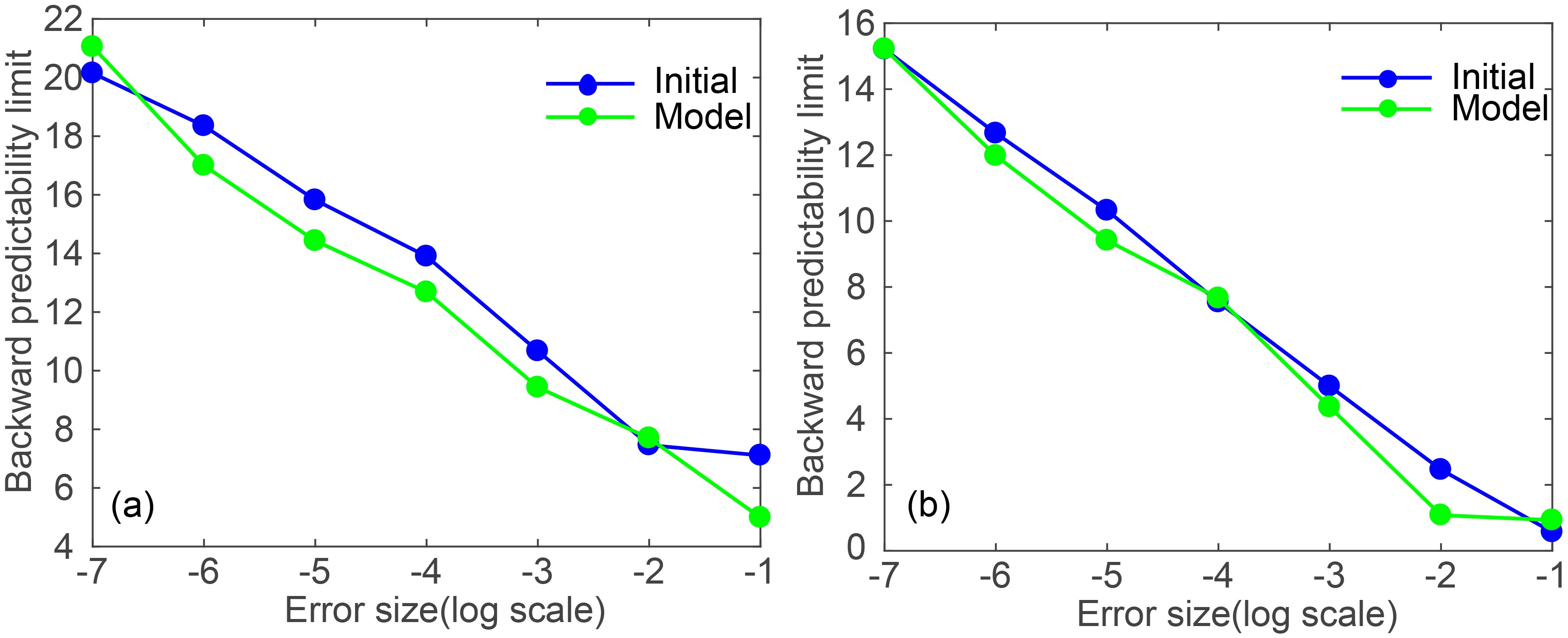 Figure7. Variation of LBPLs for the two types of errors for the states (a) (?0.54, 1.88, 26.43) and (b) (–0.32, 1.27, 24.64). Error size is given on a log10 scale.
To verify this conclusion, we selected more states to analyze. Considering that the previous 2000 consecutive states originated from the dynamically unstable regions, they are appropriate to use in the following analysis. Figure 8 shows the LBPLs induced by the two types of errors and their difference as a function of the number of states for up to 2000 states. Figure 8a shows that the LBPLs induced by initial condition and model errors have the same tendencies independent of error magnitude. As the number of specified states increases, the LBPLs first increase monotonically, then decrease monotonically, with the pattern repeating with increasing number of states. In Fig. 8b, when the magnitudes of initial condition and model errors are both 10–2 (red solid and dashed lines), the differences between model error and initial error of LBPLs are positive for the first 1339 given states, so model errors play a greater part in local backward predictability than initial condition errors, resulting in lower LBPLs. The differences are negative for the remaining 661 states, for which the initial condition errors have a greater influence on local backward predictability. Thus, the relative effect of initial condition and model errors varies with the specified state. Figure 8b also shows that the differences between the LBPLs of the same given states are different when the error magnitudes are different. This demonstrates that the error magnitude affects the relative effects of initial condition and model errors on local backward predictability.
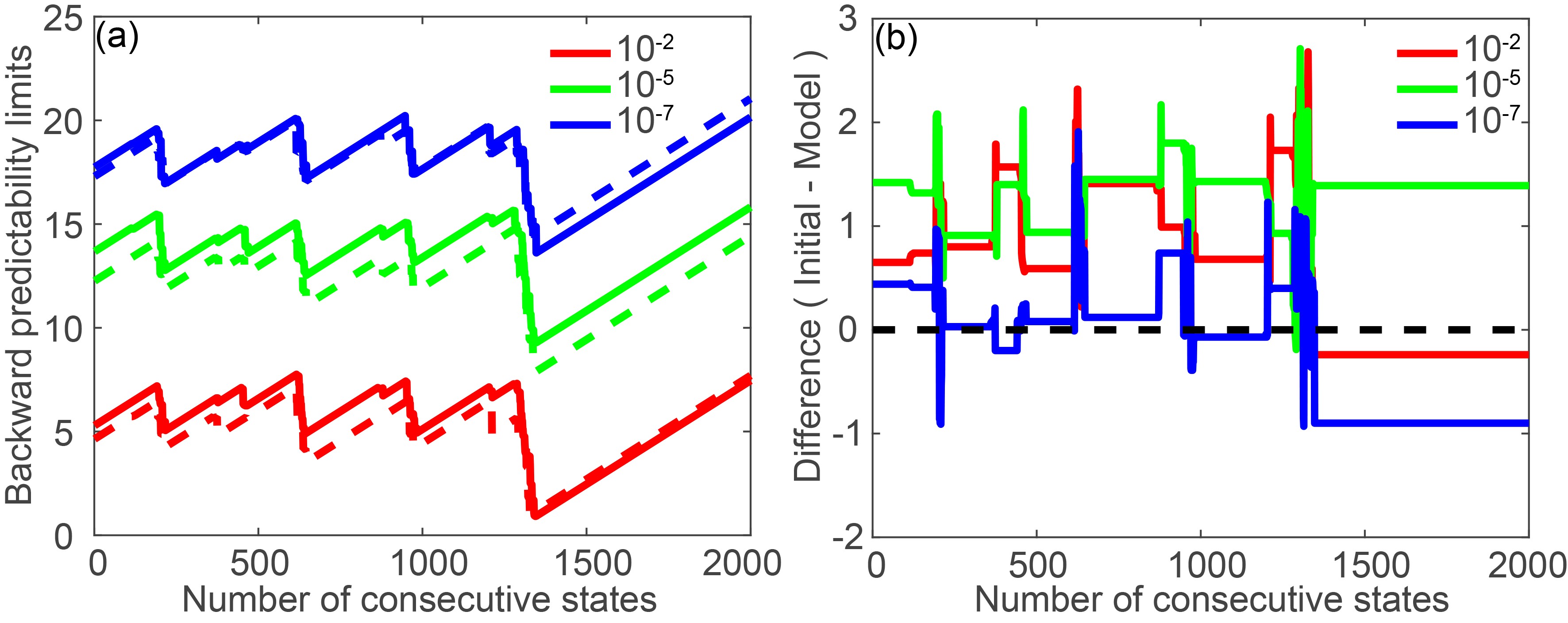 Figure8. (a) LBPLs of 2,000 consecutive states induced by initial and model errors with different magnitudes. (b) Difference (initial condition errors minus model errors) of LBPLs induced by initial and model errors of these consecutive states with different magnitudes. The solid and dashed lines in (a) represent LBPLs induced by initial condition and model errors, respectively. The red, green, and blue solid or dashed lines refer to error magnitudes of 10–2, 10–5, and 10–7, respectively (as shown by log10 values –2, –5, and –7). The black dashed line in (b) is the zero value.
Figure 9 shows the spatial distributions of LBPLs of previous 2000 consecutive states induced by the two types of errors and their differences. On an individual circular orbit, the LBPLs of given states are roughly the same, whereas the LBPLs of given states on the regime transitions are different. From the warm (cold) regime to the cold (warm) regime, the properties of states change, resulting in different predictabilities in the regime transition region. When the error magnitude is 10–2, the LBPLs of the 1336 states induced by initial condition errors are higher than those of the remaining states induced by model errors. For most of these 1336 states, the differences in the predictabilities are only slightly larger than zero, with just a small minority having larger values of up to nearly 3 time units. The large values in the local predictability difference of states are mainly distributed on the inner trajectories of the left regime. When the magnitude of errors is 10–5, the large values of difference are spread all over the attractor. When the magnitude of errors is 10–7, the large differences are found on the inner trajectories of both regimes. Therefore, the inner trajectories of left regime are frequent regions where the model errors have a larger impact on local backward predictability. But on other regions of the attractor, the initial condition errors play a more important role in local backward predictability. This also demonstrates that the relative effects of initial condition and model errors vary with the spatial locations of given states in phase space. From the spatial distributions, for the same given state with different error magnitudes, the difference between the LBPLs is not the same. This further demonstrates that the relative effects depend on the error magnitudes.
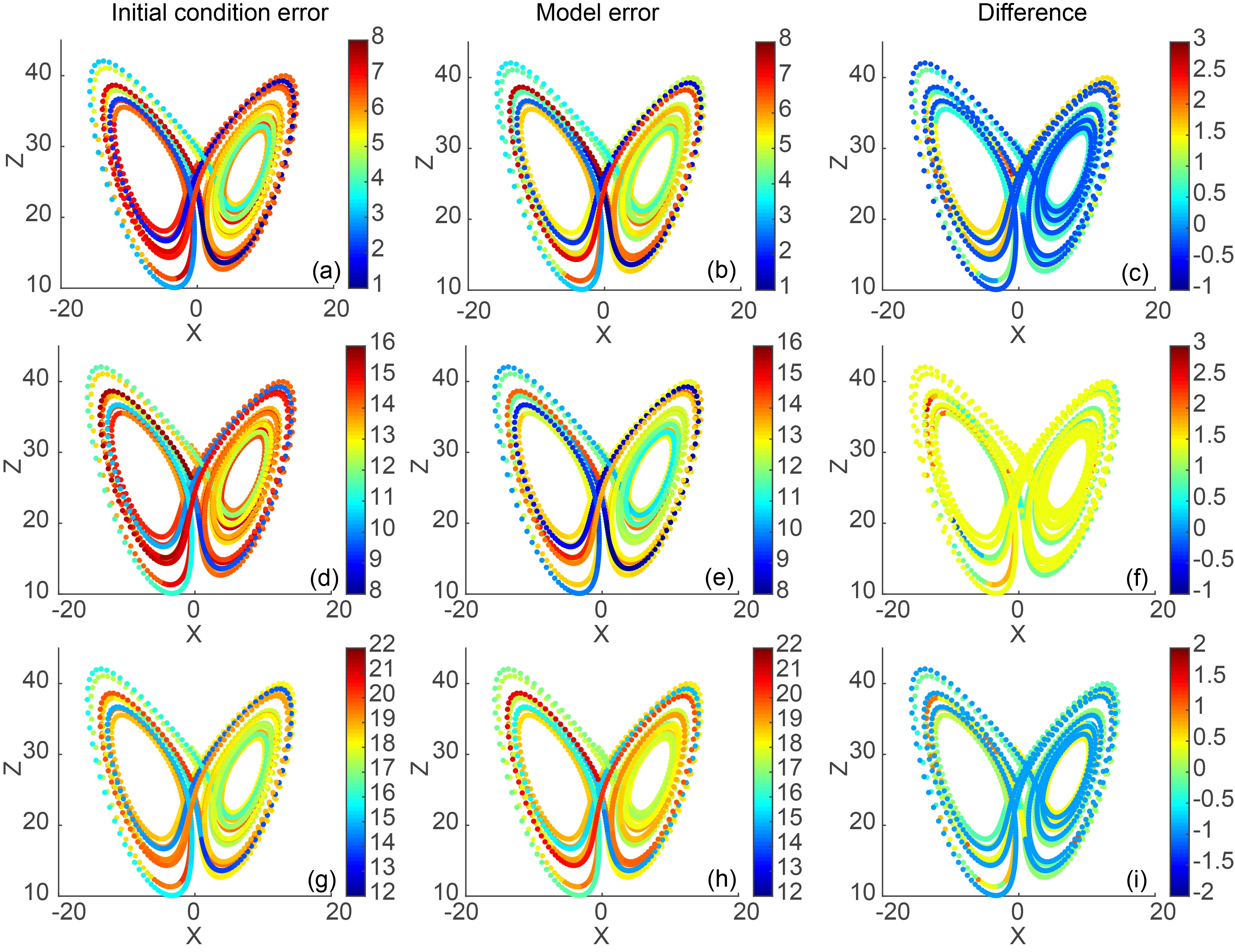 Figure9. Spatial distributions of LBPLs projected on the X–Z plane of the Lorenz attractor with initial condition and model error magnitudes of (a–c) 10?2, (d–f) 10?5, and (g–i) 10?7. The left panels only have initial condition errors in the system, the middle panels only have model errors, and the right panels show the differences between the LBPLs (initial condition errors minus model errors)induced by initial condition and model errors.
The general public and policymakers are more focused on how long in advance specific, high-impact weather events can be forecasted compared with normal weather events. Moreover, considering the rare occurrence of specific weather events, their predictabilities are unique and differ from those of normal weather events and current predictability methods fail to estimate their prediction lead time. To investigate the predictability of specific states, Li et al. (2019) proposed the BNLLE method to quantitatively estimate the LBPLs (maximum prediction lead time) of specific states.
In this work, based on the BNLLE method, we performed a theoretical study with the Lorenz model to investigate the relative effects of initial condition and model errors on the LBPLs of given states. For both types of errors, the LBPLs of given states present obvious layered structures. That is, the LBPLs of given states are roughly the same on an individual circular orbit, and are different on different circular orbits. A possible explanation of this result is that the physical properties of states on an individual circular orbit are the same, resulting in the same LBPLs. As local predictability varies with location in phase space, the LBPLs are different on different circular orbits. We also find that the local backward predictability depends on the error magnitude. For a given state, the LBPLs vary with the superimposed error magnitude. The LBPLs decrease as the magnitudes of the initial condition or model errors increase. The same magnitude of initial condition or model errors may result in different LBPLs of different given states.
Next, we compared the relative effects of initial condition and model errors on the local backward predictability of consecutive states. In the case that the difference between the LBPLs induced by initial condition and model errors is positive, our results indicate that model errors have a larger influence on local backward predictability, resulting in lower LBPLs, and vice versa. We chose 2000 consecutive states on the Lorenz attractor and calculated their LBPLs. On the whole, the differences are not always positive or always negative, indicating that the relative roles of initial condition and model errors in LBPLs vary from state to state on the dynamical trajectory. With a magnitude of 10–2, the larger differences are mainly located on the inner trajectory of the left regime. With a magnitude of 10–5, the larger differences are spread all over the attractor. With a magnitude of 10–7, the larger differences are distributed on the inner orbits of both regimes. Therefore, the inner trajectories of left regime are frequent regions where the model errors have a larger impact on local backward predictability. From the spatial distribution of LBPLs, it further demonstrates the importance of error magnitudes in the relative effects of initial condition and model errors on the local backward predictability.
From the results, the impacts of model errors are not always larger or smaller than those of initial condition errors. This is because different dynamical regions are located on the Lorenz attractor. Some regions are more sensitive to the model errors. In these regions, model errors perturbed on the states grow more rapidly, resulting in larger contributions to the loss of predictability. For different magnitudes of errors, model errors always have impacts on the inner trajectories of left regime, indicating its sensitivity to model errors. Equally, some dynamical regions are more sensitive to the initial condition errors, resulting in larger impacts on the predictability. Therefore, the results inform us that numerical weather and climate prediction models may improve prediction skills by determining the sensitive regions and reducing the corresponding errors. Lorenz (1963) pointed out that the chaotic systems were sensitive to the initial conditions. Slight differences between the two adjacent initial conditions will grow rapidly over time. Therefore, forecast errors in operational forecast are dependent on the initial conditions. However, the initial condition is not the only factor to influence the growth of forecast errors. The model errors, numerical schemes and some other sources will also influence the growth of forecast errors. In this work, we studied the impacts of model errors on the forecast error growth in the absence of initial condition errors. The findings indicate that for some cases, the model errors play a more important role in the forecast error growth. Under such circumstances, the effects of model errors on the saturation value or the limit cannot be ignored.
Although numerical models are widely used in the study of predictability, theoretical predictability methods are still necessary. The predictability limits estimated by theoretical predictability methods are complementary to those estimated by numerical models. Some research has succeeded in applying theoretical predictability methods to estimate the potential predictability limits of the real atmosphere based on observational data (e.g. Ding et al., 2010, 2015; Li and Ding, 2011). In the present work, we applied the BNLLE method using a simple theoretical model. It is our view that it is first necessary to further examine the performance of the new method BNLLE. Only if the BNLLE performs well in the simple mode, will we have confidence to apply it to more sophisticated models. In addition, this study sheds light on the relative contributions of two types of errors on local predictability of specific states, which is also beneficial to estimating the predictability of extreme events in more sophisticated models. Therefore, it is important to carry on this work. Nevertheless, the BNLLE method applied to estimating the local backward predictability of specific states in the Lorenz model is a preliminary attempt. In the future, we will apply the BNLLE method to estimate the LBPLs of extreme weather events in the real atmosphere, which may provide guidance to modelers.
Acknowledgments. This work was jointly supported by the National Natural Science Foundation of China (Grant Nos. 42005054, 41975070) and China Postdoctoral Science Foundation (Grant No. 2020M681154).
