Xuan LI¹,
Ruiqiang DING^2,3,,,
Jianping LI⁴

Corresponding author: Ruiqiang DING,drq@mail.iap.ac.cn;

1.Department of Atmospheric and Oceanic Sciences and Institute of Atmospheric Sciences, Fudan University, Shanghai 200438, China
2.Key Laboratory of Physical Oceanography, Institute for Advanced Ocean Studies, Ocean University of China and Qingdao National Laboratory for Marine Science and Technology, Qingdao 266100, China
3.State Key Laboratory of Earth Surface Processes and Resource Ecology, Beijing Normal University, Beijing 100875, China
4.Key Laboratory of Physical Oceanography/Institute for Advanced Ocean Studies, Ocean University of China and Qingdao National Laboratory for Marine Science and Technology, Qingdao 266100, China
Manuscript received: 2020-04-07
Manuscript revised: 2020-06-01
Manuscript accepted: 2020-06-12
Abstract:The backward nonlinear local Lyapunov exponent method (BNLLE) is applied to quantify the predictability of warm and cold events in the Lorenz model. Results show that the maximum prediction lead times of warm and cold events present obvious layered structures in phase space. The maximum prediction lead times of each warm (cold) event on individual circles concentric with the distribution of warm (cold) regime events are roughly the same, whereas the maximum prediction lead time of events on other circles are different. Statistical results show that warm events are more predictable than cold events.
Keywords: backward nonlinear local Lyapunov exponent,
maximum prediction lead time,
layered structure,
statistical result
摘要:本文基于向后非线性局部Lyapunov指数（backward nonlinear local Lyapunov exponent，BNLLE）方法，定量研究了Lorenz模型中冷暖事件的可预报性。研究结果显示，冷暖事件的最长提前预报时间在相空间中呈现明显的层状结构。在暖（冷）流型的每一圈层上，所有暖（冷）事件的最长提前预报时间基本一致，而在不同的圈层上，暖（冷）事件的最长提前预报时间则不同。基于统计结果表明，暖事件比冷事件更加容易预报。
关键词:冷暖事件可预报性,
向后非线性局部Lyapunov指数,
理论最长提前预报时间,

HTML

--> --> -->

Warm and cold events are closely related to the development of human society. These events influence people’s choices about the way they live their lives. Extreme warm and cold events can cause great damage to a society. The accuracy of forecasts of warm and cold events thus receives much attention. However, the chaotic nature of the atmosphere makes generating accurate long-term forecasts a challenging task. Since the pioneering work of Thompson (1957) and Lorenz (1963), much research has been conducted on the predictability of weather and climate (e.g., Mu et al., 2009; Weisheimer et al., 2011; Duan et al., 2013; Li and Ding, 2013; Duan and Hu, 2016; Lavaysse et al., 2019). However, whether warm and cold events are similarly predictable remains unknown. Islam et al. (1993) and Snyder and Zhang (2003) suggested that initial condition errors grow more rapidly in a warm environment, leading to lower predictability than in a cold environment. Other studies have indicated that warm events have a higher upper limit of predictability than cold events (e.g., Reynolds et al., 1994; Carbone et al., 2002).
Previous studies have considered the predictability of warm and cold events from both qualitative and quantitative perspectives (e.g. Leith, 1978; Chen et al., 1995; Dambacher et al., 2003; Tang et al., 2008; Li and Ding, 2011). Quantitative estimations of the predictabilities of warm and cold events are at the frontier of climate science. Some early studies employed an error doubling-time method to determine the limit of atmospheric predictability. In this method, the predictability limit is defined as the time required for small initial errors to double in size (Leith, 1965; Charney, 1966; Mintz, 1968; Smagorinsky, 1969; Lorenz, 1982). However, some researchers have pointed out that this method is affected by the numerical model being assessed (e.g., Lorenz, 1996), and the error doubling time decreases for numerical models with greater complexity and higher resolution. Dalcher and Kalnay (1987) proposed the saturation of the root-mean-square error as an indicator of predictability. However, this method also depends on the numerical model being employed. Model deficiencies have limited the widespread application of the above methods. In addition to these methods, the global Lyapunov exponent (Eckmann and Ruelle, 1985; Wolf et al., 1985; Fraedrich, 1986, 1987) and local Lyapunov exponent methods (Nese, 1989; Yoden and Nomura, 1993; Ziehmann et al., 2000) have been used to quantitatively estimate the limit of atmospheric predictability. However, these two methods assume linear error growth, whereas the atmosphere is a chaotic system for which error growth is affected by nonlinear processes. This makes existing methods less-than-ideal for predictability assessments (Mu et al., 2003). Ding and Li (2007) introduced the nonlinear local Lyapunov exponent (NLLE) method to estimate the predictability limits of the atmosphere. This method accounts for nonlinearity and provides more accurate estimates of predictability limits than methods based on the theory of linear error growth. However, this method cannot provide the maximum prediction lead time for specific states. Following the work of Ding et al. (2008), Li et al. (2019) proposed the backward nonlinear local Lyapunov exponent (BNLLE) method to estimate the maximum prediction lead time of specific states. The BNLLE method differs from traditional methods, which quantify the prediction time from a given initial state to a future state. It can estimate the prediction lead time of a specific state. Hence, the BNLLE method is particularly suited to investigations of the predictability of extreme events. The BNLLE method introduces a new means by which modelers who employ general circulation models can study the predictability of extreme events. Apart from the BNLLE method, previous studies (Mu et al., 2002; Duan and Mu, 2005; Duan and Luo, 2010) have estimated the maximum prediction lead time of events based on the conditional nonlinear optimal perturbation (CNOP) method.
This work applies the BNLLE method to an estimation of the maximum prediction lead times of warm and cold events. The relative difficulties in predicting warm and cold events are explored by comparing the predictability limits obtained using the BNLLE method. The remainder of this paper is organized as follows. Section 2 introduces the model and the BNLLE method. A quantitative estimation and comparison of the predictabilities of warm and cold events are presented in section 3. Finally, section 4 provides a summary of the results.

2

-->

2.1. Model setup

Lorenz (1963) introduced a simplified model (hereafter referred to as Lorenz63) that applies three ordinary differential equations [Eq. (1)] to study atmospheric predictability:
where $ \sigma $, r and $ b $ are constants set to 10, 28 and 8/3, respectively, and lead to the chaotic behavior of the Lorenz63 model. x, $ y $ and $ z $ in equation (1) are three variables of Lorenz63 model. The Lorenz63 model is a simple representation of the atmosphere and has been widely used in climate science (e.g., Mukougawa et al., 1991; Palmer, 1993; Evans et al., 2004; Feng et al., 2014). We use an integration time step of 0.05 time units and a fourth-order Runge?Kutta scheme to integrate the model over 45 000 steps. The first 5000 steps are used as spin-up, and the remaining 40 000 modeled states are used in the analysis.

2 -->

2.2. Backward nonlinear local Lyapunov exponent method

In an n-dimensional nonlinear dynamical system, the growth of infinitesimal initial errors $ {{\delta }}(t_0) $ can be described as
where $ {{\eta }}({{x}}({t}_{0}), {{\delta }}(t_0), \tau ) $ is a nonlinear operator that controls the growth of initial errors $ {{\delta }}(t_0) $, $ {{x}}({t}_{0}) $ represents the initial state, $ {{\delta }}(t_0+\tau ) $ denotes the errors at time $ t_0+ \tau $, and $ \tau $ is the integration time. The NLLE is defined as
The NLLE captures the nonlinear growth of initial errors, which represents an advantage over traditional methods used to study the predictability of the atmosphere, which consider only linear error growth. To quantify the predictability of state x(t₀) in a chaotic system, several error vectors (Fig. 1) are first superimposed onto x(t₀). Then, the error vectors are allowed to evolve in each direction over time $ \tau $. The NLLEs in each direction are then calculated using Eq. (3). The average nonlinear growth rate over a prescribed time $ \tau $ is thus given by
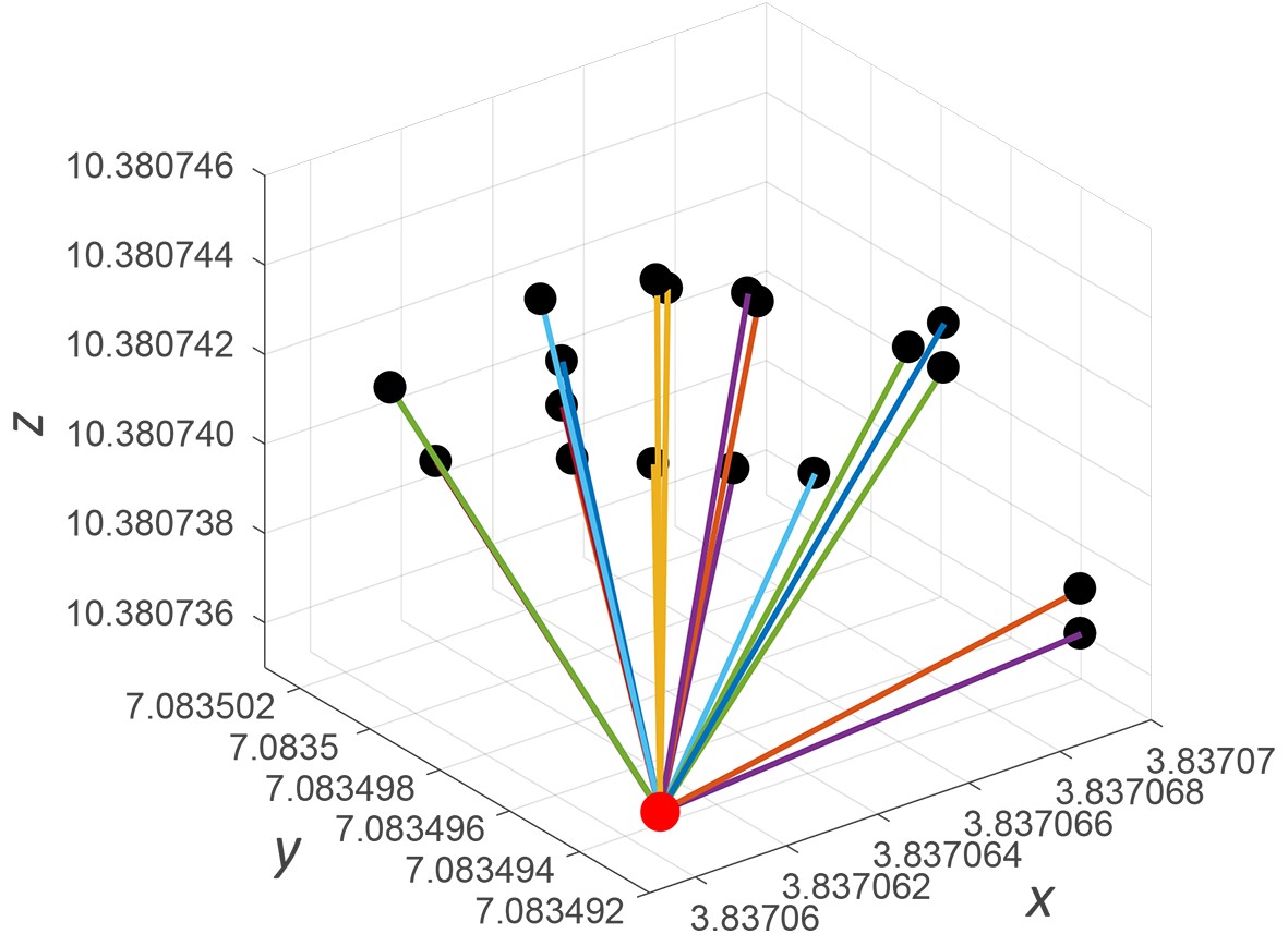Figure1. Example of 20 error vectors superimposed on the initial state ${ x}\left({t}_{0}\right)$. The red dot represents the initial state ${ x}\left({t}_{0}\right)$, and the lines connecting the red and black dots represent the error size. The magnitude of the error vectors is 10^?5.


where $ \left\langle { } \right\rangle_{{N}} $ represents the local ensemble mean of samples. The number of samples is N. The average growth of the initial errors is calculated as
In climate science, the local predictability limit of a single state x(t₀) can be represented by the time taken by initial errors to reach saturation. When the error saturates, all information of the initial state x(t₀), along with predictability, is lost. Thus, the local predictability limit can be determined once $ {\bar E}\left({{x}}\left(t_0\right),\tau \right) $ reaches saturation. The local predictability limit estimated by the NLLE method is the length of the longest possible prediction from initial state x(t₀). Thus, the NLLE method cannot provide the maximum prediction lead time for the final state x(t₀).
To estimate the maximum prediction lead time for specific final states, Li et al. (2019) proposed the BNLLE method, which is based on the NLLE method. Assume a set of time series data [ x($ {t}_{-m} $), … x($ {t}_{-1} $), x($ {t}_{0} $)]. To obtain the maximum prediction lead time for state x($ {t}_{0} $), the corresponding initial state x($ {t}_{-m} $) needs to be determined first. The corresponding initial state x($ {t}_{-m} $) must meet one condition: that errors superimposed on x($ {t}_{-m} $) evolve to saturate exactly at time $ {t}_{0} $. When the initial state x($ {t}_{-m} $) is determined, the maximum prediction lead time of state x($ {t}_{0} $) is calculated as
Unlike the NLLE method, the BNLLE method is used to calculate the maximum prediction lead time of given states by backward searches for corresponding initial states. Figure 2 shows the maximum prediction time and maximum prediction lead time for state x($ {t}_{0} $). To quantify the prediction time of state x($ {t}_{0} $), the initial errors are first superimposed on state x($ {t}_{0} $). Then, the growth of the initial errors is assessed. If the initial errors grow to reach saturation exactly at time $ {t}_{1} $, then the prediction time of state x($ {t}_{0} $) can be estimated as $ {t}_{1}-{t}_{0} $, which represents the longest effective forecast time from state x($ {t}_{0} $). To quantify the prediction lead time of state x($ {t}_{0} $), the initial errors are first superimposed on the previous state $ {{x}}\left({t}_{-1}\right) $. Then, the growth of the initial errors to time $ {t}_{0} $ is evaluated. If the initial errors reach saturation at time $ {t}_{0} $, then the maximum prediction lead time of state x($ {t}_{0} $) is estimated as $ {t}_{0}-{t}_{-1} $, which denotes the longest predictable time leading to state x($ {t}_{0} $). Therefore, the maximum prediction lead time and the maximum prediction time are two different measures of predictability of the same state. The NLLE method quantifies the maximum prediction time and the BNLLE method quantifies the maximum prediction lead time. The study of the predictability of specific states or events involves determination of the maximum prediction lead time for specific states. Thus, we apply the BNLLE method to quantify the predictabilities of warm and cold events.
Figure2. Schematic of the maximum prediction lead time (dashed line) and maximum prediction time (solid line) for state $ {{x}}\left({t}_{0}\right) $ where $ {t}_{0} $ is the time associated with given state $ {{x}}\left({t}_{0}\right) $, t₁ is the time required for the initial errors superimposed on $ {{x}}\left({t}_{0}\right) $ to reach saturation, and $ {t}_{-1} $ is the time associated with the corresponding initial state $ {{x}}\left({t}_{-1}\right) $.

2

-->

3.1. Definition of warm and cold events

Evans et al. (2004) classified the Lorenz attractor into warm and cold regimes, and studied when regime change occurs and the time spent in one regime. Warm and cold regimes represent warm and cold weather, respectively, in the real atmosphere. Figure 3 shows the warm and cold regimes of the Lorenz attractor projected on the x?y plane. For the warm regime, x and y are both greater than zero, whereas for the cold regime x and y are both less than zero. States corresponds to weather events. Of the 40 000 states, there are 17 292 states in the warm regime (i.e., warm events) and 18 534 states in the cold regime (i.e., cold events). The other 4174 states are in the regime transition region. In this work, we generate 10 000 initial error vectors randomly superimposed on each state x($ {t}_{-m} $), and the magnitudes of these initial error vectors are the same but in different directions.
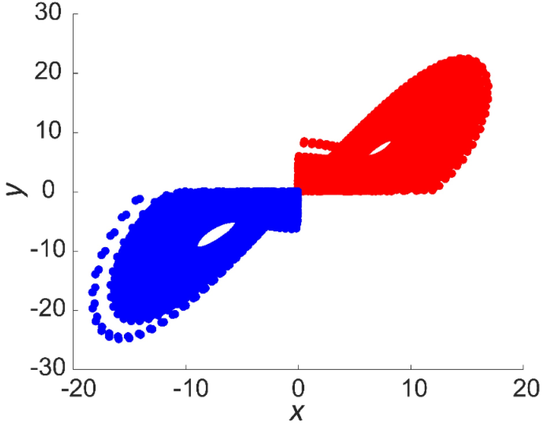Figure3. Warm (red) and cold (blue) regimes projected on the x?y plane of a Lorenz attractor.



2 -->

3.2. Maximum prediction lead times of warm and cold states

The initial error magnitude of the Lorenz63 model is set to 10^?5. We then calculate the maximum prediction lead times for all 40 000 events. Figure 4 shows the spatial distributions of maximum prediction lead times on the Lorenz attractor. Warm events are distributed over the right wing of the Lorenz attractor and cold events are distributed over the left wing. The maximum prediction lead times of warm and cold events present obvious layered structures. The maximum prediction lead times of warm (cold) events on individual circles concentric with the distribution of warm (cold) events are roughly the same. On different circles, the maximum prediction lead times are different. In addition, we find that the maximum prediction lead times of warm and cold events are similar overall, with small differences. In this work, the parameter r is 28 which is larger than 1. So the Lorenz attractor has three unstable stationary points (Mukougawa et al., 1991, Mu et al., 2002). One unstable stationary point is the origin (0, 0, 0). The other two unstable stationary points are located on ($ \sqrt{\beta (r-1)},\sqrt{\beta (r-1)},r-1 $) and ($ -\sqrt{\beta (r-1)},-\sqrt{\beta (r-1)},r-1 $), which are the centers of warm and cold regimes, respectively. The warm (cold) events on an individual orbit are circled around the unstable stationary point on the warm (cold) regime. In our opinion, the properties of all the events on an individual circle may be the same, indicating similar predictabilities of these events. So, the maximum prediction lead times of events on an individual circle are similar. Nese (1989) pointed out that the predictabilities of states vary with the phase space of the Lorenz attractor. Therefore, the predictabilities of events vary with different circles. Taking account of the two factors—the same properties of events on an individual circle and predictabilities varying with circles—the maximum prediction lead times of warm and cold events present obvious layered structures.
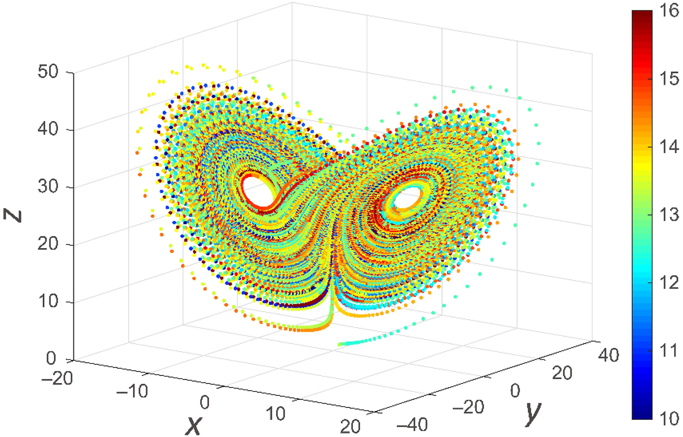Figure4. Spatial distributions of maximum prediction lead times for warm and cold regimes with initial error magnitudes of 10^?5.



2 -->

3.3. Comparison of maximum prediction lead times of warm and cold states

To further investigate which type of event is more predictable, we apply statistical information for the maximum prediction lead times of warm and cold events (Table 1). Figure 5 is a boxplot of maximum prediction lead times for warm and cold events. The largest of the maximum prediction lead times of the 17 292 warm events is slightly lower than that of the 18 534 cold events. The other four statistical variables [the first quartile (Q1), median value (Q2), the third quartile (Q3), and minimum value] of warm events are all higher than those of the cold events, indicating that warm events are more predictable than cold events.

	Minimum	Q1	Median	Q3	Maximum
Warm	10.99	12.94	13.61	14.24	16.19
Cold	10.02	12.42	13.29	14.02	16.42

Table1. Statistical information for the maximum prediction lead times of warm and cold events.


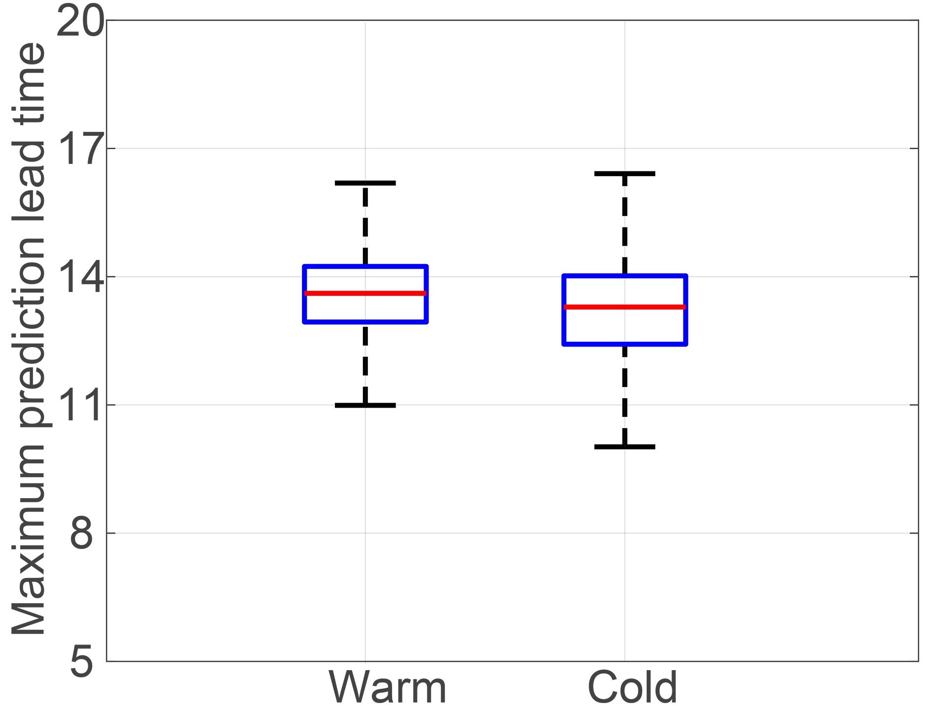Figure5. Boxplot of the maximum prediction lead time of warm and cold events with initial error magnitudes of 10^?5. Red solid lines indicate the median value (Q2). The bottoms and tops of the boxes denote the first quartile (Q1) and third quartile (Q3), respectively. The lower and upper solid horizontal lines represent the minimum value (Q1 ? 1.5IQR) and maximum value (Q3 + 1.5IQR) of the maximum prediction lead times of warm (cold) events, respectively, and IQR = Q3 ? Q1.


Figure 6 shows probability histograms of maximum prediction lead times of the two types of event under two scenarios with different initial error magnitudes. The maximum prediction lead times of warm and cold events both form Gaussian distributions. Extreme warm and cold events occur with low frequency, and thus extreme maximum prediction lead times are of low probability. For non-extreme events, the probabilities of maximum prediction lead times for warm events are generally higher than those of cold events.
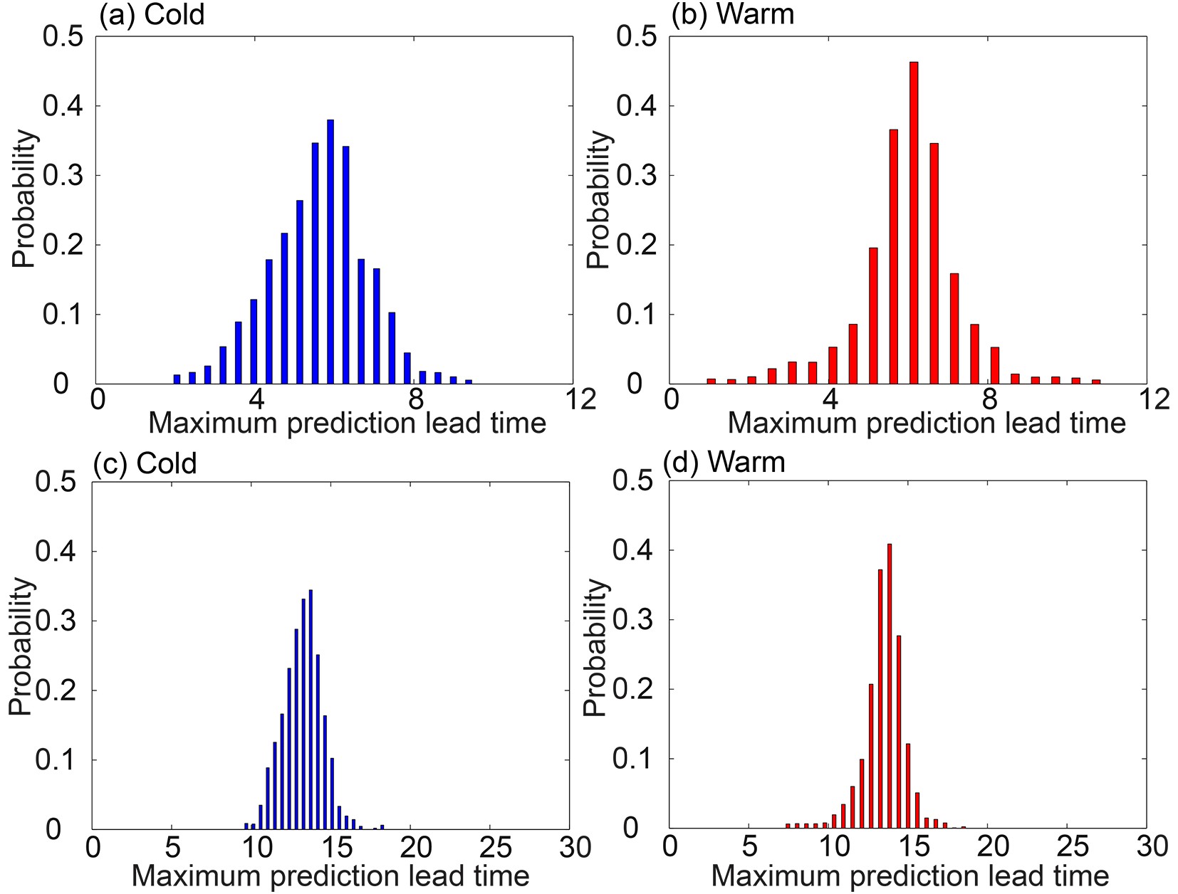Figure6. Probability histograms for maximum prediction lead times of (a, c) cold and (b, d) warm events with initial error magnitudes of (a, b) 10^?2 and (c, d) 10^?5.


Figure 7 shows probability distribution function (PDF) curves of maximum prediction lead times for warm and cold events. For both magnitudes of initial error, the probability distributions of maximum prediction lead times for warm events are shifted to longer times compared with those for cold events. The maximum prediction lead times of warm events are thus greater than those of cold events with the same probability. This demonstrates that warm events are more predictable than cold events.
Figure7. PDF curves of maximum prediction lead times for warm and cold events with initial error magnitudes of (a) 10^?2 and (b) 10^?5. Blue and red lines represent cold and warm states, respectively.

We apply the BNLLE method to quantify the maximum prediction lead times of warm and cold events in a Lorenz attractor. The BNLLE method accounts for nonlinear effects on error growth, which represents an advantage over traditional methods that assume linear error growth. Results demonstrate that the maximum prediction lead times of the two types of event present obvious layered structures in the phase space of the Lorenz system. The maximum prediction lead times of warm (cold) events on individual circles concentric with the distribution of warm (cold) events are roughly the same. However, the maximum prediction lead times on different circles are different. The properties of events on an individual orbit may be similar, resulting in similar predictability limits of these events. Because predictability varies with the phase space of the Lorenz attractor (Nese, 1989), the predictability limits of events on different circles are different. Therefore, considering the two factors, the maximum prediction lead times of warm and cold events present obvious layered structures. We also investigate which type of event is more predictable. Statistical results indicate that the Q1, median (Q2), Q3, and minimum of the maximum prediction lead times of warm events are higher than those of cold events. The distribution of maximum prediction lead times for both types of event are Gaussian with a low occurrence of extreme events. According to the probability distributions of maximum prediction lead times for warm and cold events, regardless of the magnitude of the initial error, the maximum prediction lead times of warm events are generally higher than those of cold events. Therefore, warm events are more predictable than cold events.
The atmosphere is a complex chaotic system. Warm and cold weather and climate events in the real atmosphere are more complex than those in the Lorenz63 model. In future work, we will apply the BNLLE method to the real atmosphere and further explore the relative difficulty of forecasts of warm and cold weather and climate events.
Acknowledgements. This work was jointly supported by the National Natural Science Foundation of China (Grant No. 41790474) and the National Program on Global Change and Air?Sea Interaction (GASI-IPOVAI-03 GASI-IPOVAI-06).