HTML
--> --> -->Recently, several studies focused on the capability of CMIP models in reproducing climate over China. The same conclusion was reached with a better performance for CMIP5 models, compared to their precedent generation CMIP3 models (Committee of the Third China’s National Assessment Report on Climate Change, 2015). However, there are some discrepancies for both temperature and precipitation. For instance, cold biases are generally present in western China (Guo et al., 2013; Sun et al., 2015), and overestimated precipitation in the eastern part of the Tibetan Plateau (Xu et al., 2010; Su et al., 2013). Extreme precipitation is also generally overestimated, especially in western China and in mountainous regions, while precipitation in southern China is always underestimated (Jiang et al., 2009; Jiang et al., 2012, 2015; Ou et al., 2013; Chen et al., 2014; Chen and Sun, 2014; Chen and Frauenfeld, 2014; Kusunoki and Arakawa, 2015).
Nowadays, CMIP is entering into its sixth phase (CMIP6), the models of which have higher spatial resolutions and improved parameterization schemes for major physical and biogeochemical processes of the climate system (Taylor et al., 2012; Eyring et al., 2016). Most modeling groups are releasing their new simulations with the published documentation of their model evolution from CMIP5 to CMIP6 (Kawai et al., 2019; Park et al., 2019; Wu et al., 2019; Gusain et al., 2020). However, few works have been devoted to assessing the ensemble behaviors of CMIP6 models, especially in simulating climate extremes over China. This aspect is what we want to address in the current study, with two questions framing our main motivation: (1) How does the MME (multi-model ensemble) of the CMIP6 models perform in simulating current climate extremes over China? (2) What is the level of improvement from CMIP5 to CMIP6 in this regard?
To answer these questions, simulations from 12 CMIP6 climate models were quantitatively assessed with skill-score metrics. We took all CMIP6 simulations available on ESGF as of August 2019 (when we started this work), and their performances were compared with those of the 30 existing CMIP5 models. We are aware that the 12 CMIP6 models used here are not necessarily the successors of the 30 CMIP5 models, but our goal was to assess the ensemble behaviors of the two phases of CMIP. This objective is quite distinct from that of each individual model to document changes of model constitution and performance. In this work, we want to provide a reliable scientific basis for end-users of CMIP6 simulations who are interested in the projection of future climate changes in China.
2.1. Data
As a reference from observation, we used the daily gridded dataset, CN05.1, with a resolution of 0.5° in both latitude and longitude, including four basic variables: temperature (TM), daily-maximum temperature (TX), daily-minimum temperature (TN), and precipitation. It was provided by the National Climate Center of the China Meteorological Administration based on 2416 observation stations, unevenly covering the whole of China (Wu and Gao, 2013). This dataset has been widely used in research on climate change over China (Dong et al., 2015; Xu et al., 2018).The simulated daily maximum temperature and daily minimum temperature and precipitation from 12 CMIP6 models and 30 CMIP5 models were retrieved through the data portals of the ESGF. Only the first historical realization was analyzed for each model. We used the same period, from 1961 to 2005, for both models and observations. The models used, along with their basic information, are listed in Table 1 for CMIP5 and Table 2 for CMIP6.
| Model number | Model name | Modeling center and country | Atmospheric resolution (lat × lon) |
| 1 | ACCESS1.0 | Commonwealth Scientific and Industrial Research Organization and Bureau of Meteorology(Australia) | 1.24°×1.875° |
| 2 | BCC-CSM1.1 | Beijing Climate Center, China Meteorological Administration (China) | 2.8°×2.8° |
| 3 | BCC-CSM1.1-m | Beijing Climate Center, China Meteorological Administration (China) | 1.125°×1.125° |
| 4 | BNU-ESM | College of Global Change and Earth System Science, Beijing Normal University (China) | 2.8°×2.8° |
| 5 | CanCM4 | Canadian Centre for Climate Modelling and Analysis (Canada) | 2.8°×2.8° |
| 6 | CanESM2 | Canadian Centre for Climate Modelling and Analysis (Canada) | 2.8°×2.8° |
| 7 | CCSM4 | National Center for Atmospheric Research (USA) | 0.94°×1.25° |
| 8 | CMCC-CM | Centro Euro-Mediterraneo per I Cambiamenti Climatici(Italy) | 0.75°×0.75° |
| 9 | CMCC-CMS | Centro Euro-Mediterraneo per I Cambiamenti Climatici(Italy) | 1.875°×1.875° |
| 10 | CSIRO-Mk3-6-0 | Commonwealth Scientific and Industrial Research Organization in collaboration with Queensland Climate Change Centre of Excellence (Australia) | 1.875°×1.875° |
| 11 | CNRM-CM5 | Centre National de Recherches Météorologiques–Centre Européen de Recherche et de Formation Avancée en Calcul Scientifique (France) | 1.4°×1.4° |
| 12 | FGOALS-g2 | LASG, Institute of Atmospheric Physics, Chinese Academy of Sciences and Center for Earth System Science, Tsinghua University(China) | 3°×2.8° |
| 13 | FGOALS-s2 | LASG, Institute of Atmospheric Physics, Chinese Academy of Sciences(China) | 1.67°×2.8° |
| 14 | GFDL-CM3 | NOAA Geophysical Fluid Dynamics Laboratory (USA) | 2.0°×2.5° |
| 15 | GFDL-ESM2G | NOAA Geophysical Fluid Dynamics Laboratory (USA) | 2.0°×2.5° |
| 16 | GFDL-ESM2M | NOAA Geophysical Fluid Dynamics Laboratory (USA) | 2.0°×2.5° |
| 17 | HadCM3 | Met Office Hadley Centre(United Kingdom) | 2.5°×3.75° |
| 18 | HadGEM2-CC | Met Office Hadley Centre(United Kingdom) | 1.24°×1.875° |
| 19 | HadGEM2-ES | Met Office Hadley Centre(United Kingdom) | 1.24°×1.875° |
| 20 | IPSL-CM5A-LR | L’Institut Pierre-Simon Laplace(France) | 1.875°×3.75° |
| 21 | IPSL-CM5A-MR | L’Institut Pierre-Simon Laplace(France) | 1.26°×2.5° |
| 22 | MIROC4h | National Institute for Environmental Studies,The University of Tokyo (Japan) | 0.56°×0.56° |
| 23 | MIROC5 | National Institute for Environmental Studies,The University of Tokyo (Japan) | 1.4°×1.4° |
| 24 | MIROC-ESM | National Institute for Environmental Studies,The University of Tokyo (Japan) | 2.8125°×2.8125° |
| 25 | MIROC-ESM-CHEM | National Institute for Environmental Studies,The University of Tokyo (Japan) | 2.8125°×2.8125° |
| 26 | MPI-ESM-LR | Max Planck Institute for Meteorology (Germany) | 1.875°×1.875° |
| 27 | MPI-ESM-MR | Max Planck Institute for Meteorology (Germany) | 1.875°×1.875° |
| 28 | MPI-ESM-P | Max Planck Institute for Meteorology (Germany) | 1.875°×1.875° |
| 29 | MRI-CGCM3 | Meteorological Research Institute (Japan) | 1.125°×1.125° |
| 30 | NorESM1-M | Norwegian Climate Centre (Norway) | 1.8725°×2.5° |
Table1. Model names, modeling centers and countries, as well as the atmospheric resolutions, of 30 CMIP5 global climate models.
| Model number | Model name | Modeling center and country | Atmospheric resolution (lat × lon) |
| 1 | BCC-CSM2-MR | Beijing Climate Center, China Meteorological Administration (China) | 1.125°×1.125° |
| 2 | BCC-ESM1 | Beijing Climate Center, China Meteorological Administration (China) | 2.8°×2.8° |
| 3 | CNRM-CM6-1 | Centre National de Recherches Météorologiques–Centre Européen de Recherche et de Formation Avancée en Calcul Scientifique (France) | 1.4°×1.4° |
| 4 | CNRM-ESM2-1 | Centre National de Recherches Météorologiques–Centre Européen de Recherche et de Formation Avancée en Calcul Scientifique (France) | 1.4°×1.4° |
| 5 | EC-Earth3-Veg | EC-EARTH consortium | 0.7°×0.7° |
| 6 | GFDL-CM4 | NOAA Geophysical Fluid Dynamics Laboratory (USA) | 1°×1.25° |
| 7 | GFDL-ESM4 | NOAA Geophysical Fluid Dynamics Laboratory (USA) | 1°×1.25° |
| 8 | IPSL-CM6A-LR | L’Institut Pierre-Simon Laplace(France) | 1.26°×2.5° |
| 9 | MRI-ESM2-0 | Meteorological Research Institute (Japan) | 1.125°×1.125° |
| 10 | NESM3 | Nanjing University of Information Science and Technology(China) | 1.875°×1.875° |
| 11 | SAM0-UNICON | Seoul National University(Republic of Korea) | 0.94°×1.25° |
| 12 | UKESM1-0-LL | Met Office Hadley Centre(UK) | 1.25°×1.875° |
Table2. Model names, modeling centers and countries, as well as the atmospheric resolutions, of 12 CMIP6 global climate models.
Different climate indices from different models and observations were firstly calculated on their native grids. Then, to facilitate the intercomparison, a bilinear interpolation scheme was used to interpolate all indices to a common 1° × 1° grid.
Monthly vertical velocity together with meridional wind and specific humidity were also used in our study to search for the possible reasons behind the better performance of CMIP6-MME to reproduce precipitation in South China. The corresponding variables from the NCEP–NCAR reanalysis, with a resolution of 2.5°, were used as a reference for the same period, 1961–2005. All models were interpolated to a 2.5° × 2.5° grid to facilitate the intercomparison.
2
2.2. Climate indices
In this work, we consider 10 climate indices, including the annual average temperature and nine extreme indices defined by the Expert Team on Climate Change Detection and Indices (| Name | Abbreviation | Definition | Units |
| Avg TM | Tav | Annual average value of daily temperature (TM) | °C |
| Max TX | TXx | Annual maximum value of daily maximum temperature (TX) | °C |
| Min TN | TNn | Annual minimum value of daily minimum temperature (TN) | °C |
| Cold nights | TN10p | Percentage of days when TN < 10th percentile | % |
| Warm days | TX90p | Percentage of days when TX > 90th percentile | % |
| Total precipitation | Prcptot | Annual total precipitation in wet days (RR ≥ 1 mm) | mm |
| Heavy precipitation | R95p | Annual total precipitation from days > 95th percentile | mm |
| Precipitation intensity | Sdii | Total wet days precipitation divided by the number of wet days | mm d?1 |
| Consecutive dry days | CDD | Maximum number of consecutive days with RR <1 mm | d |
| Extremely heavy rain days | R20mm | Annual count of days with RR ≥ 20 mm | d |
Table3. Names, abbreviations, definitions, and units of climate indices used in the study.
2
2.3. Evaluation method
32.3.1. Taylor diagram
To evaluate the overall skill in reproducing the spatial pattern of the present-day climate indices, the Taylor diagram and Taylor skill score (TS) (Taylor, 2001; Wang et al., 2018) were used. The Taylor diagram provides a concise statistical summary of the degree of correlation (PCC; pattern correlation coefficient), centered root-mean-square error (RMSE), and the ratio of spatial standard deviation (RSD). The similarity between observations and simulations can be quantified by their correlation and the amplitude of the variability. A perfect simulation would be one with a centered RMSE equal to 0 and both the PCC and RSD close to 1. The TS is a combined measure and calculated as:where R is the spatial correlation coefficient between the simulation and observation; R0 is the maximum correlation coefficient attainable (here we use 0.999); and σsm and σso are the standard deviations (SDs) of the simulated and observed spatial patterns, respectively. The score equals 1 for a perfect match between the model and observation, and 0 for an inverse model performance.
3
2.3.2. Interannual variability skill score
The method to quantitatively express the interannual variability skill score (IVS) is the same as employed in Chen et al. (2011):where σtm and σto denote the interannual SDs of the model simulations and observations, respectively. Smaller IVS values indicate better performance of the simulation.
3.1. Temperature indices
33.1.1. Climatology
In order to evaluate the capability of models in reproducing temperature indices over China, Fig. 1 shows the box-and-whisker plots and the spatial distribution of biases between simulations (CMIP6-MME and CMIP5-MME) and observation from 1961 to 2005. All the box-and-whisker plots use the commonly used convention with upper and lower limits of the box indicating the 75th and 25th percentile values, the horizontal line in the box indicating the median, the dot in the box indicating the mean, and the whiskers showing the 90th and 10th percentile values. It can be seen that CMIP6-MME has a general cold bias throughout the country. The areal-mean bias of CMIP6-MME for annual mean temperature (Tav), maximum daily maximum temperature (TXx), and minimum daily minimum temperature (TNn) in the whole of China is ?1.64°C, ?0.45°C and ?4.51°C, respectively. Large cold biases are located over the Tibetan Plateau, where the local bias is more than 4°C for Tav and 8°C for TNn. Compared with CMIP5-MME, CMIP6-MME does not present obvious differences for Tav or TNn. Except for TXx, the general warm bias (0.93°C) in CMIP5-MME becomes a general cold bias (?0.45°C) in CMIP6-MME (Figs. 1e and f). Regions where biases in CMIP6-MME are lower than in CMIP5-MME and their difference is statistically significant at the 5% level are dotted in the middle panels. The dotted areas in Fig. 1e represent the simulated bias for TXx from CMIP6-MME is significantly reduced in North China and parts of Xinjiang. The dotted areas are mainly located in Xinjiang for Tav and TNn, which indicates the bias over Xinjiang is also reduced in CMIP6-MME (Figs. 1b and h). Figure1. Box-and-whisker plots (left column) and the spatial pattern of biases (simulation minus observation) in CMIP6-MME (middle column, red) and CMIP5-MME (right column, blue) of temperature indices for the historical period, 1961–2005 (units: °C, °C, °C, %, %). The areal-mean bias (Bias) over China and the intermodel SD of the difference averaged over the country (middle and right column) are given on the top of each panel. From top to bottom are (a–c) Tav, (d–f) TXx, (g–i) TNn, (j–l) TN10p and (m–o) TX90p, respectively. The dotted areas in the middle panels represent regions where biases in CMIP6-MME are lower than in CMIP5-MME and the difference is statistically significant at the 5% level.
Generally speaking, it is difficult to evaluate model performances with percentile indices because the mean threshold exceedance rate in the base period is approximately the same for all models and observations (Sillmann et al., 2014; Chen and Sun, 2015). The calculations of these percentile indices for the models and observations are implemented over the standard base period of 1961–90, and the climatic mean analyses are calculated over the period of 1961–2005. There is a systematic overestimation from CMIP6-MME for cold nights (TN10p), but a systematic underestimation for warm days (TX90p). CMIP5-MME shows similar spatial characteristics for TN10p. However, the simulated bias is basically distributed as a north–south dipole for TX90p, with negative bias in the north and positive bias in the south.
Apart from biases measuring the deviation of models from observation, the intermodel spread is also considered as an important assessment for CMIP models, since it indicates the degree of consensus across the climate modeling community, and ultimately serves as a surrogate to measure uncertainty in climate models, especially for the projection of future climate. With this idea in mind, we next evaluate the SD among models for CMIP5 and CMIP6 respectively. We follow what was done in Jiang et al. (2016) and display the areal-mean SD over the whole of China in the upper part of each relevant panel in Fig. 1. The intermodel SD for all CMIP6 models (CMIP6-twelve) is generally smaller than that of all CMIP5 models (CMIP5-thirty) for most temperature indices (except TNn). We believe that such a difference is not significant, since CMIP5 (30 members) is more diverse than CMIP6 (12 members). Results (not shown) from a subset of six CMIP6 models (CMIP6-six) and their CMIP5 predecessors (CMIP5-six) do not permit us to conclude significant differences either, which confirms that the intermodel spread is quite comparable between CMIP5 and CMIP6.
Taylor diagrams and TSs are also used to further evaluate the overall skills of models in reproducing the spatial pattern of temperature indices. Figure 2 shows the Taylor diagrams for the 12 CMIP6 and 30 CMIP5 models and their MME against observations, combined with the TS histograms of their MME. The majority of models (both CMIP5 and CMIP6) have PCCs greater than 0.85 for Tav, TXx, and TNn. This indicates that the coupled models perform well in simulating the spatial distribution of these indices, with RSDs between 0.75 and 1.25 and RMSEs less than 0.5. The result from the MME is furthermore much better than for individual models. The PCC and TS for each index of both CMIP5-MME and CMIP6-MME are above 0.94, the RSD is close to 1, and the RMSE close to 0.25. Compared with CMIP5, CMIP6 models also show some improvements for TXx, with larger PCCs and TSs. If we examine TN10p and TX90p, presented in the lower panels in Fig. 2, all models (both CMIP5 and CMIP6) show relatively poor performances, with PCCs below 0.5. Even the MME is not good enough, with PCCs below 0.6 and TSs below 0.3. This feature has also been revealed by previous studies (e.g., Chen and Sun, 2015).
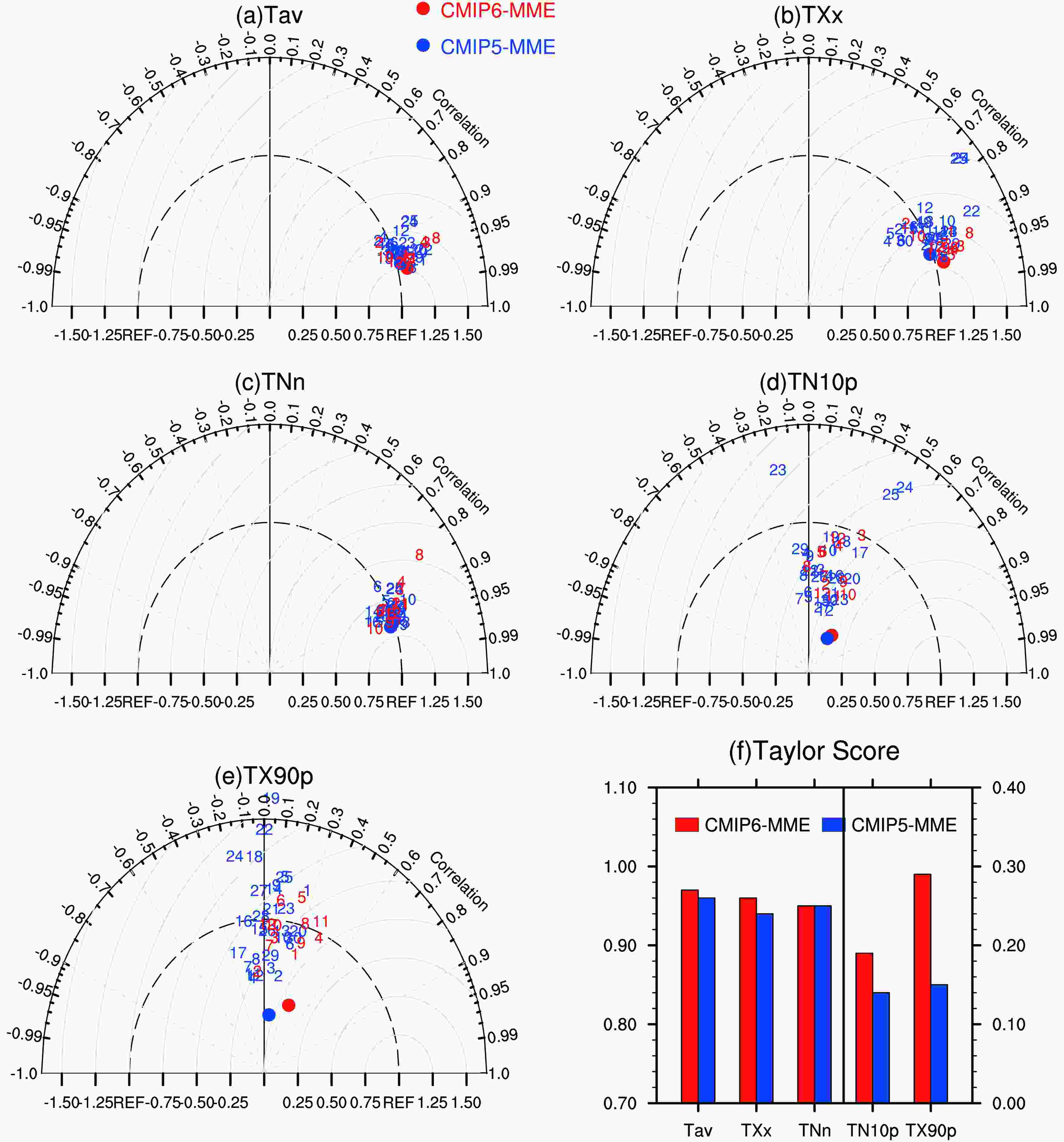 Figure2. Taylor diagrams (a–e) and skill scores in terms of TS (f) showing the performance of models (CMIP6 in red, CMIP5 in blue) in simulating climatological fields over China for five temperature indices. Angular axes show pattern correlation coefficients between simulated and observed fields; radial axes show the spatial centered RMSE (normalized against the observed). Blue and red numbers indicate CMIP5 and CMIP6 models listed in Tables 1 and 2. The larger solid circles represent the MME. The scale of Tav, TXx, TNn is on the left y-axis, and that of TN10p and TX10p is on the right y-axis.
We also compared the subset of CMIP6-six models with their CMIP5-six predecessors by using similar Taylor diagrams (results not shown), and the performance of models for temperature indices was generally similar between CMIP6 and CMIP5. It was even noticeable that, for TNn, CMIP6 models presented some degradation, mainly due to the poor performance of IPSL-CM6A-LR. The capabilities of their ensemble means (MME) in reproducing the climatological temperature indices were also close to each other. For the subset of six affiliation-identified simulations, we also performed a further analysis as presented in Sillmann et al. (2013), providing a compact graphical overview of models’ performances relative to each other. The basic calculation is the RMSE relative to the observed climatology, and then the RMSE is subtracted and normalized by the median value among the models to compare and for each parameter. Such a processing allows half of the models with positive values and the second half with negative values. It is clear that models with negative values perform better compared to those with positive values. Results for temperature indices are shown in Fig. 3, wherein colors are used to show the magnitude of the normalized relative RMSE; warm colors indicate models in the bad half, and cold colors indicate models in the good half. From a visual inspection, we can easily conclude that the six affiliated CMIP6 simulations are not distinguishable from their CMIP5 counterparts.
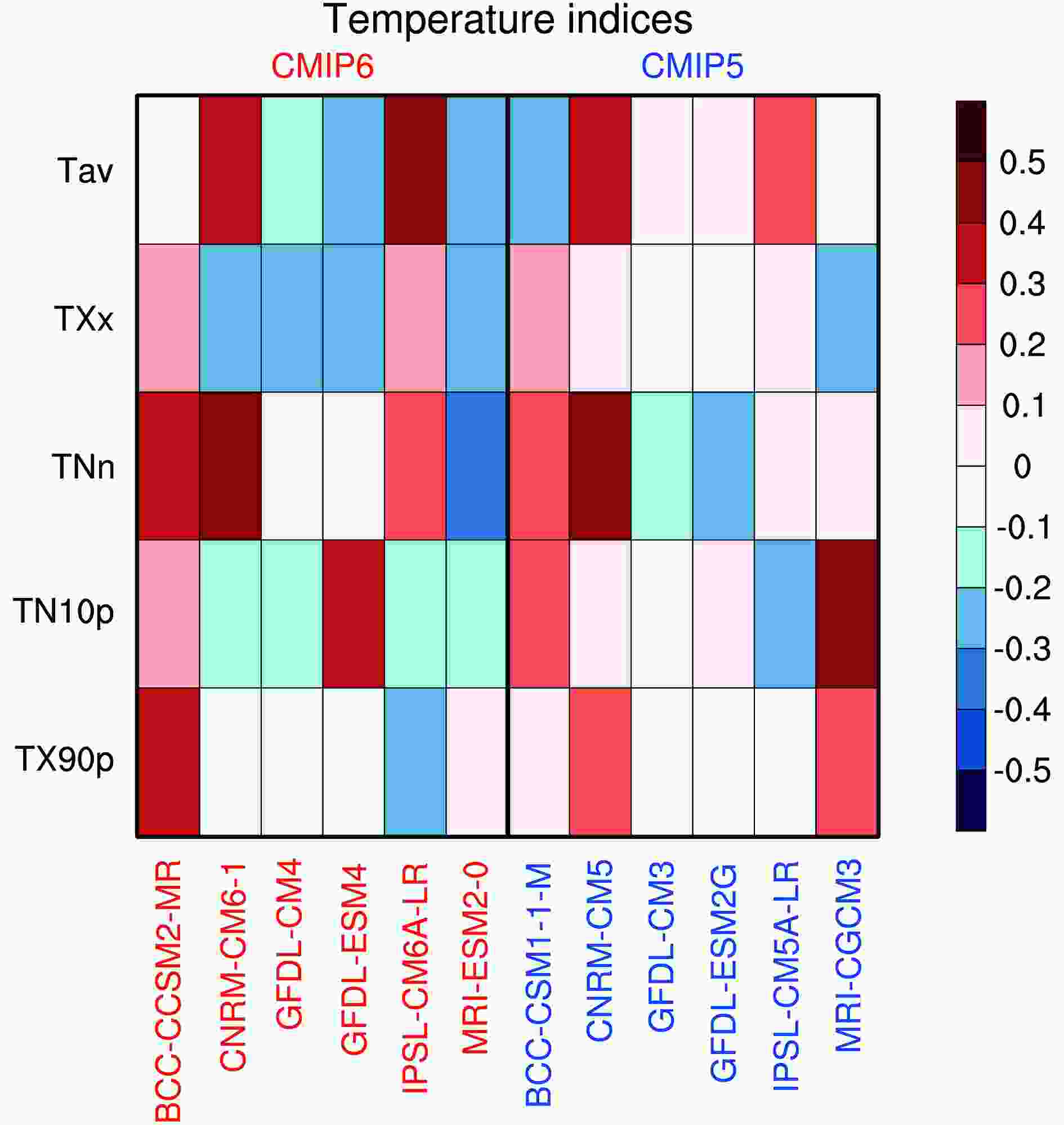 Figure3. Portrait diagram of relative spatially averaged RMSEs in the 1961–2005 climatologies of temperature indices simulated by CMIP6 (red) and CMIP5 (blue) models from the same institution with respect to the observation.
Generally speaking, both CMIP6-MME and CMIP5-MME exhibit good capabilities in simulating the spatial distribution of Tav, TXx and TNn, but have difficulties in reproducing TN10p and TX90p. CMIP6-MME still has cold biases over the Tibetan Plateau for Tav and TNn, which may be related to the complex physical characteristics of the underlying surface of the plateau. Climate models, with their relatively coarse resolution, cannot depict the steep terrain of the plateau and the complex characteristics of the underlying surface (IPCC, 2007, 2013; Gao et al., 2008). However, compared with CMIP5-MME, the warm biases for TXx in some regions of Northwest China have significantly reduced in CMIP6-MME. The capability of CMIP6-MME to simulate the spatial distribution of TN10p and TX90p is still relatively poor, but shows some improvement in comparison with CMIP5-MME. Considering all temperature indices as a whole, we can conclude that the simulation performance regarding their spatial pattern is similar in CMIP6 and CMIP5, and the intermodel spread is at a comparable level in CMIP5 and CMIP6.
3
3.1.2. Interannual variability
The performance in simulating the temporal variation is also a very important factor to measure the capability of models. The IVS defined in section 2.3.2 is used here to quantify the similarity of the interannual variability between simulated and observed indices. Figure 4 gives the IVS histogram of models for five temperature indices in China. Both CMIP6 and CMIP5 models can realistically simulate the interannual variation of temperature indices, with a mean IVS less than 1. The mean IVS of Tav, TN10p and TX90p from CMIP6 models is 0.26, 0.33 and 0.25, respectively. The mean IVS of Tav, TN10p and TX90p from CMIP5 models is 0.35, 0.28 and 0.31, respectively. CMIP6 models perform better than CMIP5 models for TXx; the mean IVS from CMIP6 and CMIP5 models is 0.51 and 0.91, respectively. Considering all temperature indices, we can again conclude that the simulation of interannual variation of different temperature indices is of similar performance between CMIP6 and CMIP5. Figure4. Skill scores in terms of IVS for the five temperature indices in CMIP6 (red) and CMIP5 (blue) models over China. The filled bars show the ensemble mean, and the error bars represent ranges of one SD (1σ) among models. Asterisks (**) indicate that the differences between CMIP6 and CMIP5 models are significant at the 95% confidence level based on the t-test, with an asterisk (*) for 90%.
2
3.2. Precipitation indices
33.2.1. Climatology
The simulation of precipitation is more challenging for models as it depends closely on the parameterization of complex physical processes and their implementation in models. Major challenges are linked to surface properties (topography, coastline, vegetation) that lead to much greater spatial heterogeneity at regional scales (IPCC, 2007, 2013). Figure 5 shows the box-and-whisker plots and the spatial distribution of biases between simulation and observation for different precipitation indices for the common period from 1961 to 2005. The precipitation indices simulated by CMIP6-MME are generally overestimated, except for consecutive dry days (CDD). The areal-mean relative bias of CMIP6-MME for total precipitation (Prcptot), heavy precipitation (R95p), and precipitation intensity (Sdii), in the whole of China, is 79%, 85% and 21%, respectively. The largest wet bias is located over the Himalayan mountains and the eastern part of the Tibetan Plateau, where the local bias is more than 600 mm for Prcptot, 150 mm for R95p, and 3 mm d?1 for Sdii, respectively (Figs. 5b, e and h). The subset ensemble means from six models with identified affiliation, CMIP5-six and CMIP6-six, perform in a very similar way as in Fig. 5.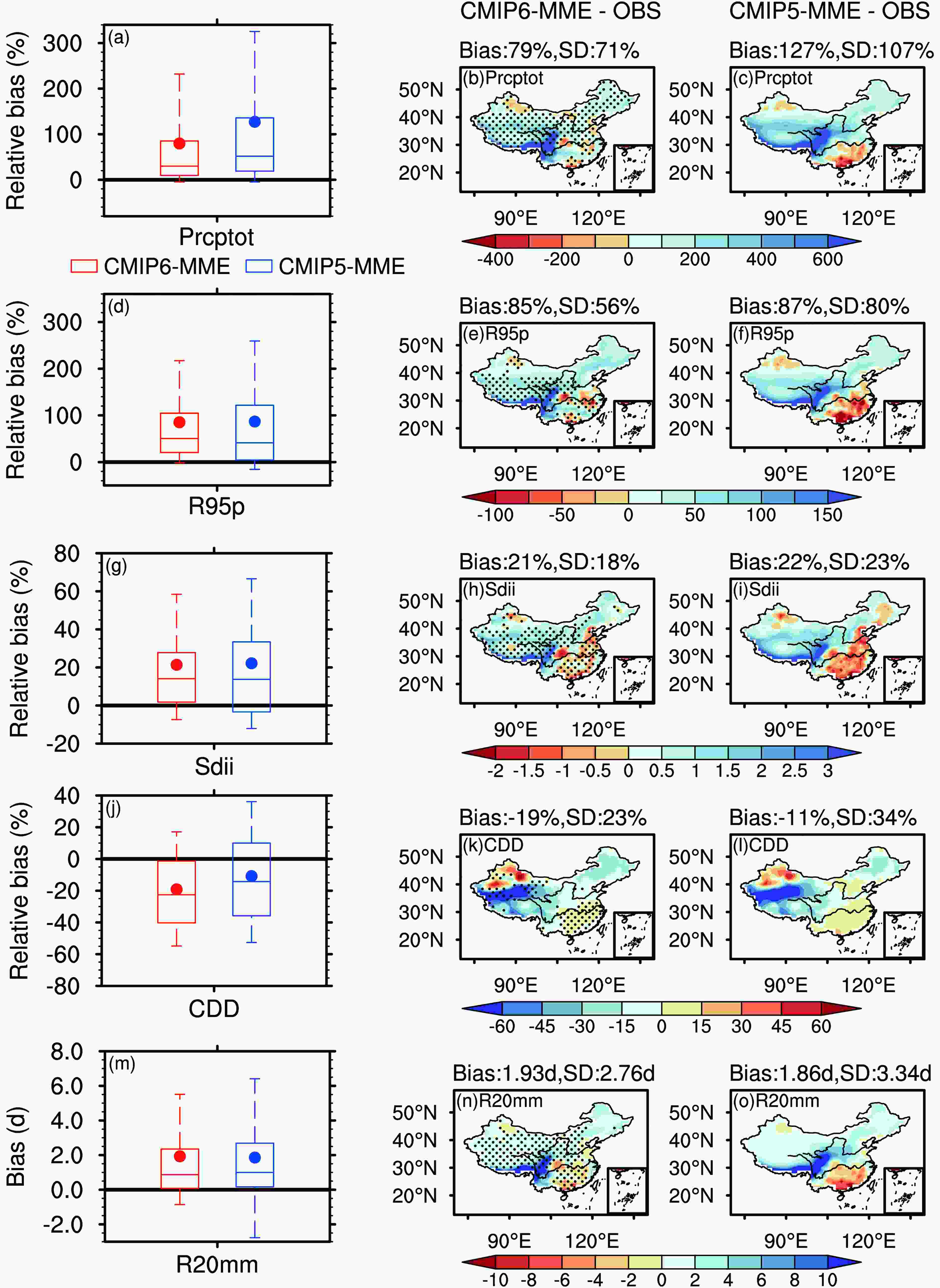 Figure5. As in Fig. 1. but for (a–c) Prcptot, (d–f) R95p, (g–i) Sdii, (j–l) CDD and (m–o) R20mm (units: mm, mm, mm d?1, d, d). The areal-mean percentage bias (Bias) over China and the intermodel SD of the difference in percentage averaged over the country (middle and right column) are given on the top of each panel (but with bias and intermodel SD of the difference for R20mm; units: d).
CMIP6-MME shows significant improvements in the simulation of precipitation indices compared with CMIP5-MME, except for CDD, which has similar performance in the two ensembles. For Prcptot (Fig. 5a), the areal-mean bias has been reduced from 127% in CMIP5-MME to 79% in CMIP6-MME. Similarly, the median relative bias has also been reduced, from 51% (CMIP5-MME) to 30% (CMIP6-MME). Although the high skewness of the precipitation distribution leads to different behaviors, both the mean and median show a clear improvement from CMIP5-MME to CMIP6-MME. CMIP5-MME shows obvious dry biases in the south of the Yangtze River for Prcptot, R95p and Sdii (negative bias for extremely heavy rain days, R20mm), while dry (negative) biases are significantly decreased in CMIP6-MME (Figs. 5b, e, h and n, dotted areas). This feature is also observed with the subset ensemble results. The biases of Prcptot (exceeding ?400 mm) and R95p (exceeding ?100 mm) in CMIP5-MME over South China are reduced to less than ?200 mm and ?50 mm in CMIP6-MME, respectively. The Tibetan Plateau is also within the dotted area in Fig. 5 (middle column), which indicates the large wet bias here is reduced in CMIP6-MME.
CDD does not show obvious improvement in CMIP6-MME, with overestimation in Xinjiang and in southern China, but underestimation in other regions, especially in the Kunlun Mountains (north part of the Tibetan Plateau), where the bias is over 60 days (Fig. 5k). The areal-mean bias of CDD over the whole of China is ?15.7 days. The spatial distribution from CMIP5-MME is similar, and the areal-mean bias over China is ?13.1 days.
Unlike temperature indices showing inconclusive variation between CMIP5 and CMIP6 in terms of intermodel spread, precipitation indices display a clearer trend of reduced intermodel spread from CMIP5 to CMIP6. This is true for the total ensembles (Fig. 5) and the subset ensembles (results not shown).
Figure 6 shows Taylor diagrams and TSs as a concise representation of performance with respect to all precipitation indices. Most models (for both CMIP5 and CMIP6) have PCCs between 0.6 and 0.9 for Prcptot, R95p and Sdii, indicating that the coupled models have certain capability in simulating the spatial distribution of these indices. For Sdii especially, the PCCs are all larger than 0.7 and the RMSEs smaller than 0.75. However, they are generally less skillful in simulating CDD and R20mm. For CDD in particular, the PCCs of almost all models (both CMIP5 and CMIP6) are smaller than 0.75, and the RSDs are further away from 1. The model spread of most precipitation indices is much larger than that of temperature indices (Tav, TXx and TNn) in both CMIP5 and CMIP6. The MME is generally better than individual models, with a larger PCC and smaller RMSE.
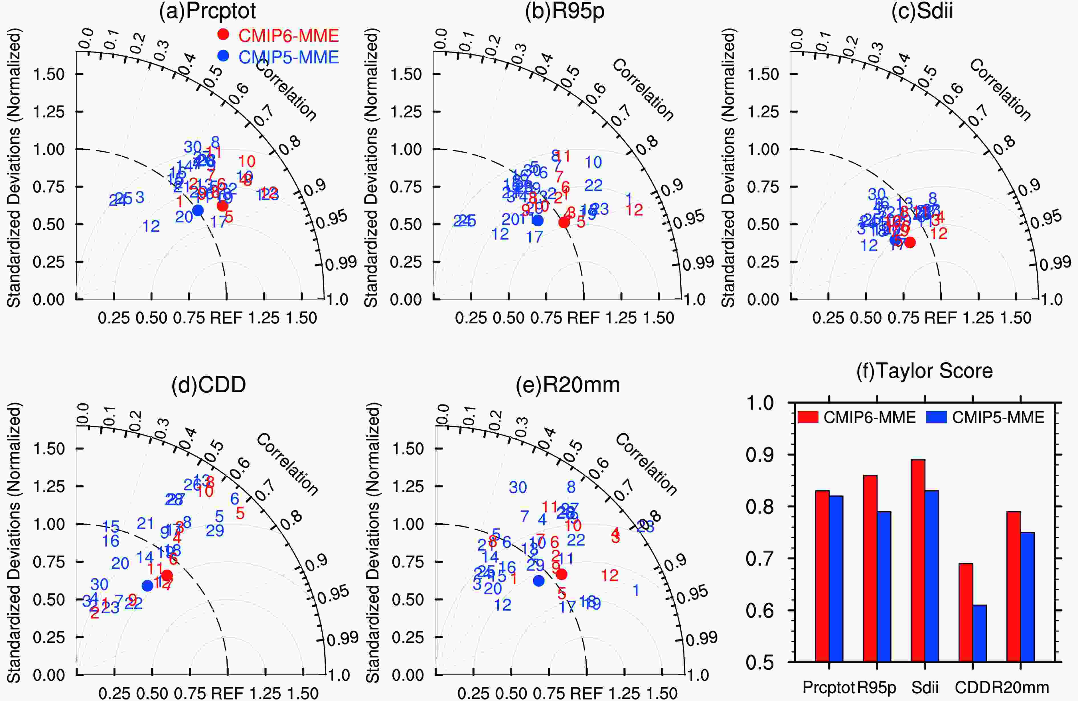 Figure6. As in Fig. 2. but for five precipitation indices.
The performance of CMIP6 models has clearly improved compared with that of CMIP5 models, especially for R95P and Sdii. The PCC for R95p/Sdii has increased from 0.80/0.87 (CMIP5-MME) to 0.86/0.92 (CMIP6-MME); and the TS for R95p/Sdii has also increased, from 0.79/0.83 to 0.86/0.89, respectively. The RSD from CMIP6-MME is also closer to 1, and the RMSE closer to 0, which indicates that the performance in simulating the spatial pattern of R95p and Sdii is more significantly improved than for other indices from CMIP6-MME. CDD also presents certain improvements from CMIP5 to CMIP6, with the TS increasing from 0.61 (CMIP5-MME) to 0.69 (CMIP6-MME). The subset ensemble CMIP6-six also shows significant improvements compared to its counterpart, CMIP5-six, for most precipitation indices, including the ensemble average. A few models (e.g., BCC-CSM2-MR, GFDL-CM4 and GFDL-ESM4) even systematically outperform their CMIP5 predecessors for all precipitation indices. The capability of climate models to reproduce climatological precipitation indices over China rises from CMIP5 to CMIP6. This improvement is also visible in Fig. 7, which presents a portrait diagram of multiple precipitation indices from the subset ensembles, with dominant blue colors for CMIP6-six and dominant orange colors for CMIP5-six.
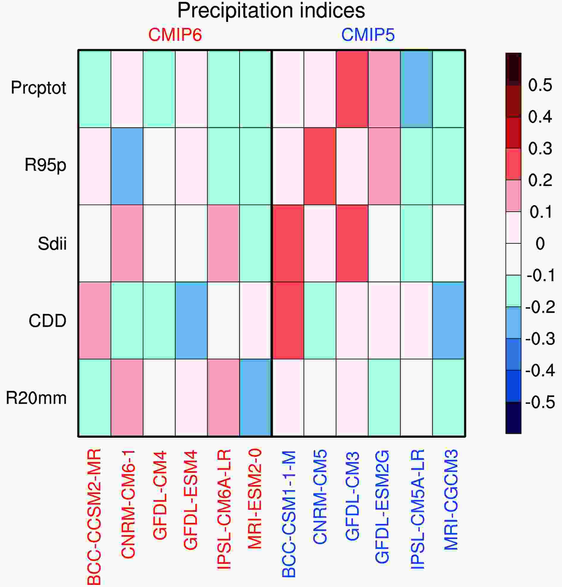 Figure7. As in Fig. 3. but for five precipitation indices.
3
3.2.2. Interannual variability
Figure 8 shows the mean IVS histogram of models for the five precipitation indices averaged over China. For all indices, the mean IVS from CMIP6 models is lower than that of CMIP5 models. Taking Sdii as an example, the mean score from CMIP6 models is 0.91, and the mean score of CMIP5 models is 1.18. The IVSs of other indices are larger, but CMIP6 models have smaller mean values than CMIP5 models.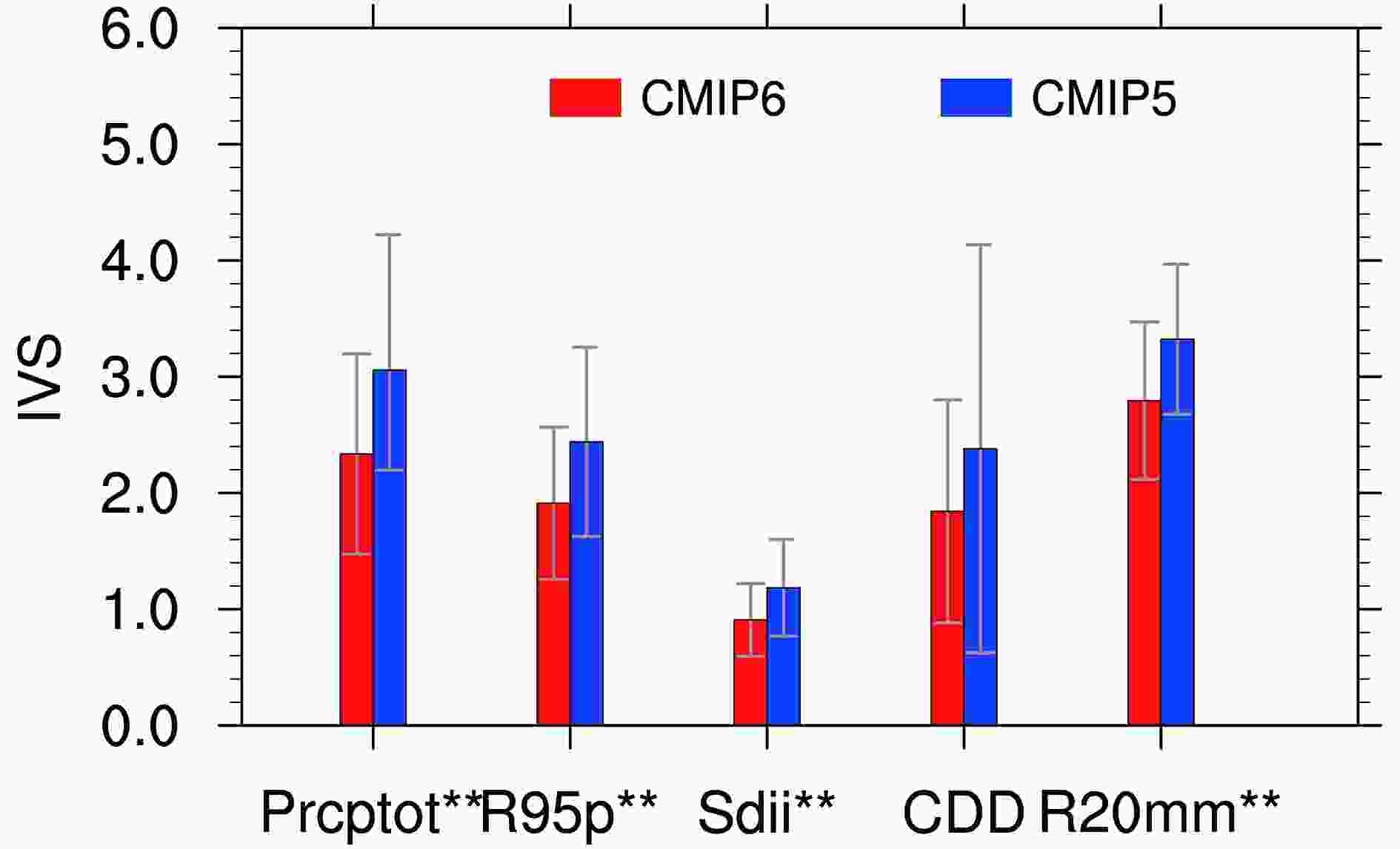 Figure8. As in Fig. 4. but for five precipitation indices.
Generally speaking, both CMIP6-MME and CMIP5-MME have certain capabilities in simulating precipitation indices, but are not as good as they are simulating temperature indices (Tav, TXx and TNn). The models are more skillful in reproducing temperature than precipitation, which is also consistent with previous studies (IPCC, 2013; Kusunoki and Arakawa, 2015). For different precipitation indices, the performance of the models is different, with the best for Sdii and the worst for CDD. Considering all precipitation indices, we can conclude that CMIP6 models are superior to CMIP5 models in simulating both the spatial distribution and interannual variability, and have smaller intermodel spreads than CMIP5 models. In particular, the dry bias of mean and extreme precipitation in southern China is largely reduced in CMIP6-MME. However, CMIP6-MME still has wet biases for Prcptot, R95p and Sdii in the eastern Tibetan Plateau, but these wet biases are smaller than those of CMIP5-MME. This improvement may be partly attributable to the higher model resolution and better description of physical and chemical processes in CMIP6 models (Eyring et al., 2016). CMIP6 models generally have improved convective parameterization schemes and cloud physics processes (Cao et al., 2018; Wu et al., 2019), and append the indirect effects posed by aerosols onto the formation of clouds and precipitation (Voldoire et al., 2019; Wu et al., 2019).
To further investigate possible causes for the better performance of CMIP6-MME in reproducing precipitation in South China, the regional atmospheric circulation patterns from the two MMEs are compared with the NCEP reanalysis. Considering the fact that June–August (JJA) is the main season for precipitation occurrence in China, Fig. 9 shows the difference in meridional circulation and specific humidity (shaded) zonally averaged within 110°–120°E in summer. As shown in Fig. 9 (middle column), compared with NCEP, CMIP5-MME presents strong descent around 30°N. CMIP5-MME also shows less water vapor over South China, so there is a large dry bias over the region (Figs. 5b and e). For CMIP6-MME (Fig. 9, left column), however, the zone of strong descent is northward-shifted compared to CMIP5-MME. CMIP6-MME also shows a little more water vapor and weak ascent around 22°N compared to NCEP. Therefore, the dry bias is reduced in South China in CMIP6-MME (Figs. 5a and d). Furthermore, compared with CMIP5-MME, CMIP6-MME presents stronger ascent between 22°N and 30°N. CMIP6-MME also shows more water vapor over South China (Fig. 9, right column). Hence, the stronger ascent accompanied by more moisture over South China in CMIP6-MME contributes to the reduced dry biases over the region.
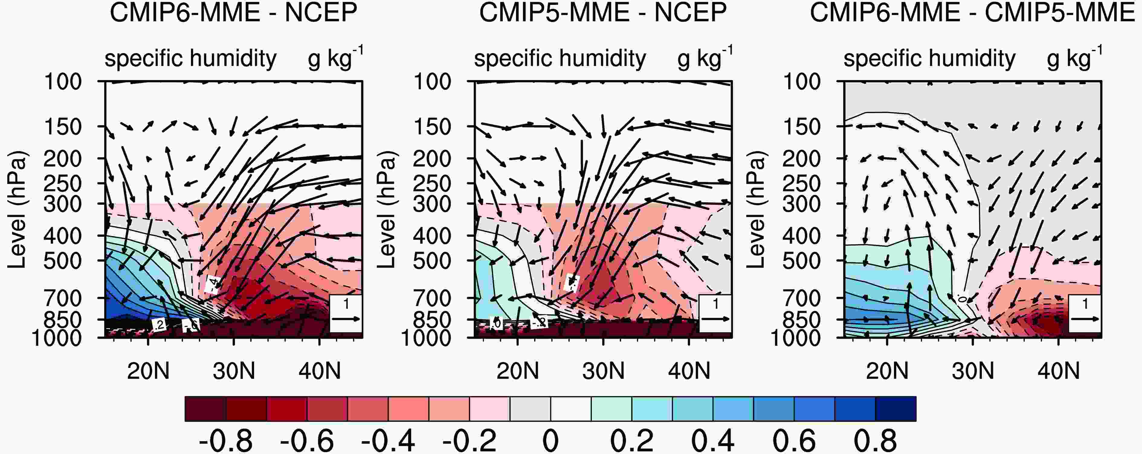 Figure9. Differences in meridional overturning circulation (vectors; units: m s?1) and specific humidity (shading; units: g kg?1; increase in blue, decrease in red) zonally averaged within 110°–120°E for the historical period, 1961–2005, in summer (JJA). From left to right are CMIP6-MME minus NCEP, CMIP5-MME minus NCEP, and CMIP6-MME minus CMIP5-MME. The abscissa is the latitude and the ordinate is the pressure level (units: hPa) [specific humidity has fewer levels (only to 300 mb) from NCEP].
Both CMIP6 and CMIP5 models show good performance in simulating the climatological pattern and the interannual variation for temperature indices over China. The spreads among models for most temperature indices are at a comparable level in CMIP5 and CMIP6. CMIP6-MME and CMIP5-MME have very good capabilities in reproducing Tav, TXx and TNn, with PCCs and TSs larger than 0.94. However, they have difficulties in successfully reproducing TN10p and TX90p. CMIP6-MME generally shows slight improvements in comparison with CMIP5-MME. The large warm biases of CMIP5-MME for TXx in parts of Northwest China are significantly reduced in CMIP6-MME. However, the large cold bias of CMIP5-MME over the Tibetan Plateau still exist in CMIP6-MME for Tav (exceeding ?4°C) and TNn (exceeding ?8°C).
The performance of the CMIP6 and CMIP5 models in simulating precipitation indices is not as good as that in simulating temperature indices (Tav, TXx and TNn). For different precipitation extremes, the capability of the models is also different, with the best for Sdii and the worst for CDD. CMIP6 models have a smaller intermodel spread than CMIP5 models for most precipitation indices, which implies a slightly larger consensus in CMIP6 historical simulations. We hope that there will also be smaller uncertainties when we deal with the projection of future climate within CMIP6. Compared with CMIP5-MME, CMIP6-MME shows significant improvements in simulating both the climatological pattern and the interannual variation for precipitation indices, except for CDD, which remains at the same level. The areal-mean bias for Prcptot is reduced from 127% (CMIP5-MME) to 79% (CMIP6-MME). The dry biases for mean and extreme precipitation in southern China are also largely reduced in CMIP6-MME. However, CMIP6-MME still has wet biases for Prcptot, R95p and Sdii in the eastern Tibetan Plateau, although these wet biases are smaller than those of CMIP5-MME.
The dry biases for precipitation indices (Prcptot, R95p and Sdii) over South China are tightly related to the strong descent and weak water vapor content over the region. CMIP6-MME, with ascent and moist air over South China, is able to produce more precipitation, and to reduce the dry biases over there. CMIP6 models generally have higher horizontal resolutions and improved physical parameterizations (convection, radiation, cloud, land surface, etc.), which together certainly contribute to the apparent improvement, although we are unable currently to determine the precise cause. In eastern China, convective precipitation is the main type of precipitation, so deficiencies in convection parameterization are likely to cause the systematic errors in precipitation simulation, especially for extreme precipitation (Li et al., 2012; Rosa and Collins, 2013; Mehran et al., 2014; Jiang et al., 2015). CMIP6 models have generally improved convection parameterization schemes and cloud physics (Cao et al., 2018; Wu et al., 2019), which can also partly explain the significant improvement in precipitation simulation over southern China.
It should be pointed out that CMIP6-MME still has large biases for temperature indices over the Tibetan Plateau and Northwest China. The precipitation indices in western China are also not well simulated; in particular, there are large wet biases over the eastern Tibetan Plateau. Topographic forcing has an important influence on the simulation of climate (Zhou et al., 2009; Song et al., 2013). It would be relatively difficult for models to reproduce the effects of the complex topography in western China (Chen et al., 2012).
Due to the temporarily limited number of available CMIP6 models, evaluation of more CMIP6 models still needs to be carried out in the future. However, based on the results of the 12 CMIP6 models in this paper, the improvement in precipitation simulation compared with CMIP5 models is of great significance for providing more comprehensive climate information to end-users or policymakers. The climate projection results of the Scenario Model Intercomparison Project (Scenario MIP) for CMIP6 (O’Neill et al., 2016) are also being gradually released, which will allow us to assess future climate change projections from CMIP6 models. Based on this assessment, we would recommend with confidence to use CMIP6 results for future climate projection in China.
Acknowledgements. We wish to thank the three anonymous reviewers, whose valuable comments and suggestions helped us to improve our manuscript. We would like to acknowledge the World Climate Research Programme’s Working Group on Coupled Modelling, which is responsible for CMIP. We thank the climate modeling groups for producing and making their model outputs available. This research was supported by the National Key Research and Development Program of China (Grant Nos. 2017YFA0603804 and 2018YFC1507704) and the Natural Science Foundation of China (Grant No. 41805048).
