HTML
--> --> -->The term “rapid cyclogenesis” was first coined by Bergeron (1954), and refers to the rapid drop of central sea level pressure (SLP) of severe storms that deepen by at least 24 hPa within 24 hours. Thus, the unit for the deepening rate of the central SLP of a cyclone is termed “Bergeron” (1 Bergeron = 1 hPa h?1). The first quantified EC definition was given by Sanders and Gyakum (1980), and referred to a surface weather low-pressure system whose central SLP falls at least 1 Bergeron within 24 hours, adjusted geostrophically to 60°N. Later, according to the latitude of maximum EC occurrence over the Northern Hemisphere, the latitude in the EC definition was modified by several researchers. For example, Roebber (1984) adjusted 60°N to 42.5°N, while Gyakum et al. (1989) and Zhang et al. (2017) adjusted 60°N to 45°N. Additionally, with improvements in the temporal resolution of data, Yoshida and Asuma (2004) and Zhang et al. (2017) modified the EC definition by using 12-hourly pressure change instead of 24-hourly pressure change.
Previous studies have indicated that ECs are predominantly cold-season weather systems (Sanders and Gyakum, 1980; Roebber, 1984; Chen et al., 1992; Wang and Rogers, 2001; Yoshida and Asuma, 2004), as their occurrence peaks in the winter season (Sanders and Gyakum, 1980; Yoshida and Asuma, 2004; Allen et al., 2010; Zhang et al., 2017). Sanders and Gyakum (1980) showed that the number of ECs over the Northern Hemisphere is at a maximum in January, followed by February and December. In addition, many ECs occur in November. Chen et al. (1992) also documented that the number of ECs decreases successively in January, December, March and February. Yoshida and Asuma (2004) indicated that ECs over the northwestern Pacific can be classified into three types: the Okhotsk?Japan Sea type (O?J type), the Pacific Ocean?Land type (PO-L type), and the Pacific Ocean–Ocean type (PO?O type). The number of O-J-type cyclones is at a maximum in November, whereas PO-L-type cyclones peak in December and February, and PO-O-type cyclones are most frequent in January. The number of ECs over the northwestern Pacific is also the most in the winter season. The statistical results of Allen et al. (2010) showed that most ECs occur over the Northern Hemisphere in the winter season. By using National Centers for Environmental Prediction (NCEP) Final Analysis data during the cold season (October?April) from 2000 to 2015, Zhang et al. (2017) investigated ECs over the northern Pacific. According to the spatial distribution of their maximum deepening rate locations, ECs over the Northern Pacific were further classified into five regions: the Japan?Okhotsk Sea, the northwestern Pacific, the West-Central Pacific, the East-Central Pacific, and the northeastern Pacific. Additionally, these ECs had four intensity categories: weak, moderate, strong, and super.
Due to the differences of employed data, the spatial distributions of ECs have differed slightly from study to study. For ECs over the northern Pacific, several studies (Sanders and Gyakum, 1980; Wang and Rogers, 2001; Allen et al., 2010) have indicated that their spatial distribution extends eastward from the east of Japan, spanning the whole northern Pacific. Sanders and Gyakum (1980, their Fig.3) found that ECs mainly occur over the ocean during the cold season, using three cold-season (September 1976 to May 1979) datasets. They pointed out that there are four most-frequent occurrence areas of ECs over the northern Pacific: the area from the east of Japan to 165°E; the area from 170°E to 180°; the area from 175°W to 160°W; and the northeastern Pacific (from 150°W to 140°W). Chen et al. (1992, their Fig.4) investigated the climatology of explosive cyclogenesis off the East Asian coast, using 30 years (1958?87) of surface station data. They indicated that there are two favorable areas for explosive cyclone deepening: one over the east of the Japan Sea; and the other over the north Pacific, which is close to the warm Kuroshio Current. Wang and Rogers (2001, their Fig.1) also found that there are two significant EC frequent-occurrence areas—over the northwestern Pacific (from 125°E to 180°) and over the northeastern Pacific (around 145°W)—using the twice-daily, 2.5° × 2.5° gridded analysis data from the European Centre for Medium-Range Weather Forecasts (ECMWF) from January 1985 to March 1996. However, the number of ECs over the northeastern Pacific was found to be less than that over the northwestern Pacific. By using 2.5°×2.5° NCEP2 reanalysis data from 1979 to 2008, Allen et al. (2010, their Fig. 6a) pointed out that the distribution of ECs over the North Pacific can be classified into three frequent-occurrence areas: the east of Japan (from 140°E to 155°E); the area from 170°E to 180°; and the area from 155°W to 135°W.
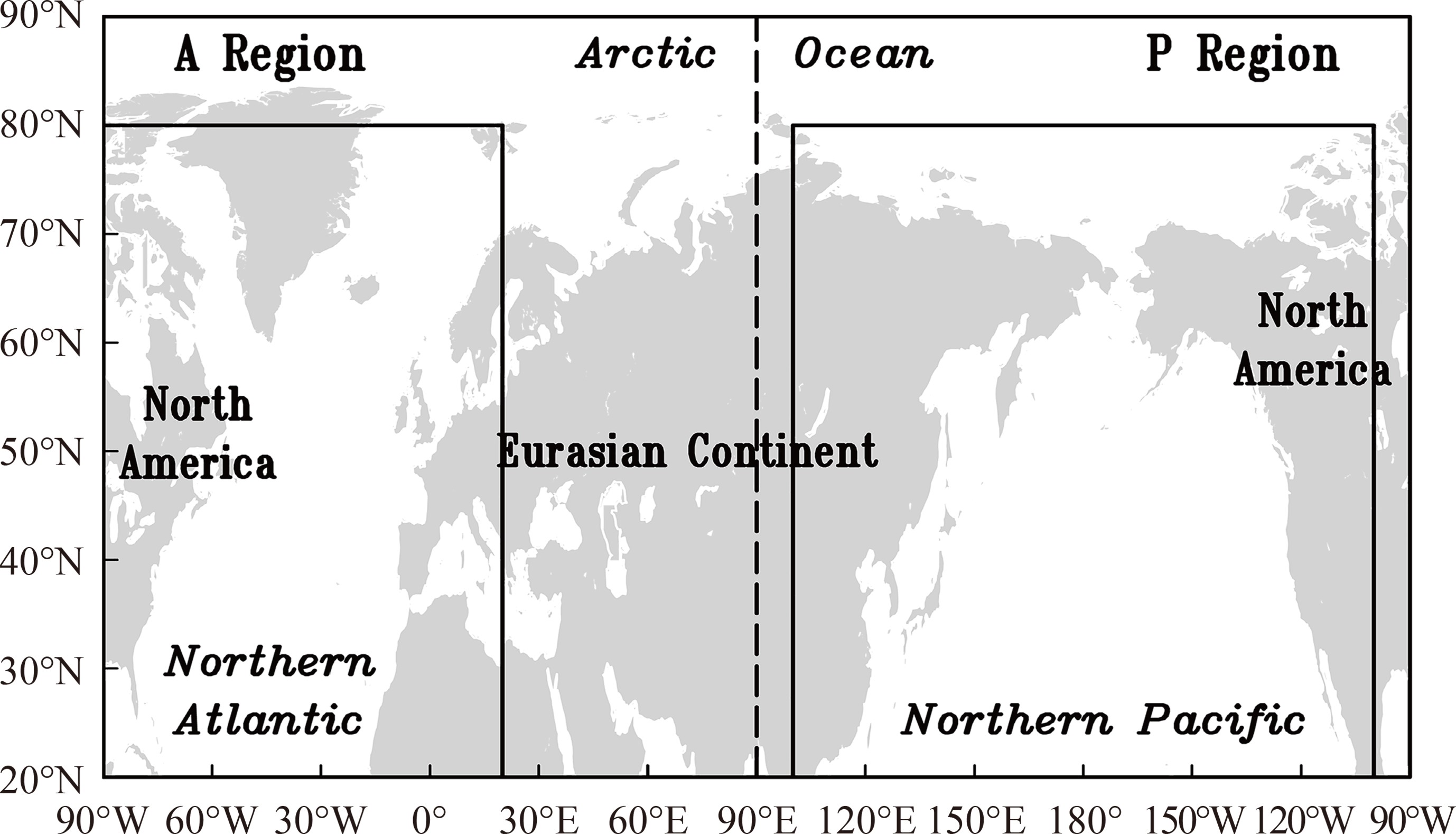 Figure1. Geographic map of the study domain over the Northern Hemisphere. The left-hand domain represents the A region and the framed area represents the northern Atlantic region. The right-hand domain represents the P region and the framed area represents the northern Pacific region.
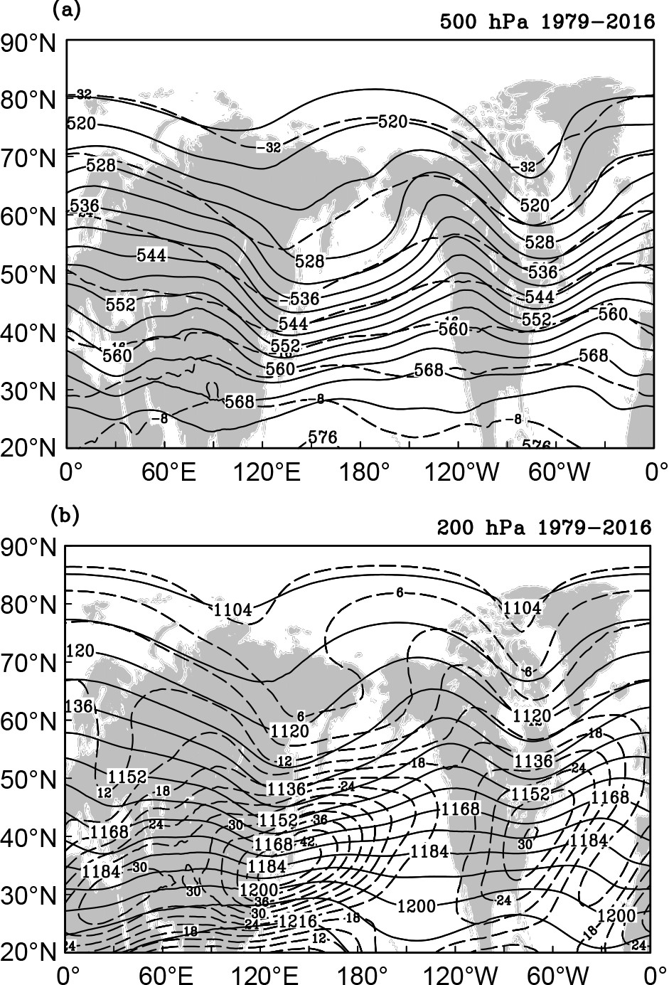 Figure3. Mean atmospheric circulation in the Northern Hemisphere from 1979 to 2016: (a) 500-hPa geopotential height (solid lines; interval: 40 gpm) and air temperature (dashed lines; interval: 4°C); (b) 200-hPa geopotential height (solid lines; interval: 80 gpm) and isotach (dashed lines; interval 3 m s?1).
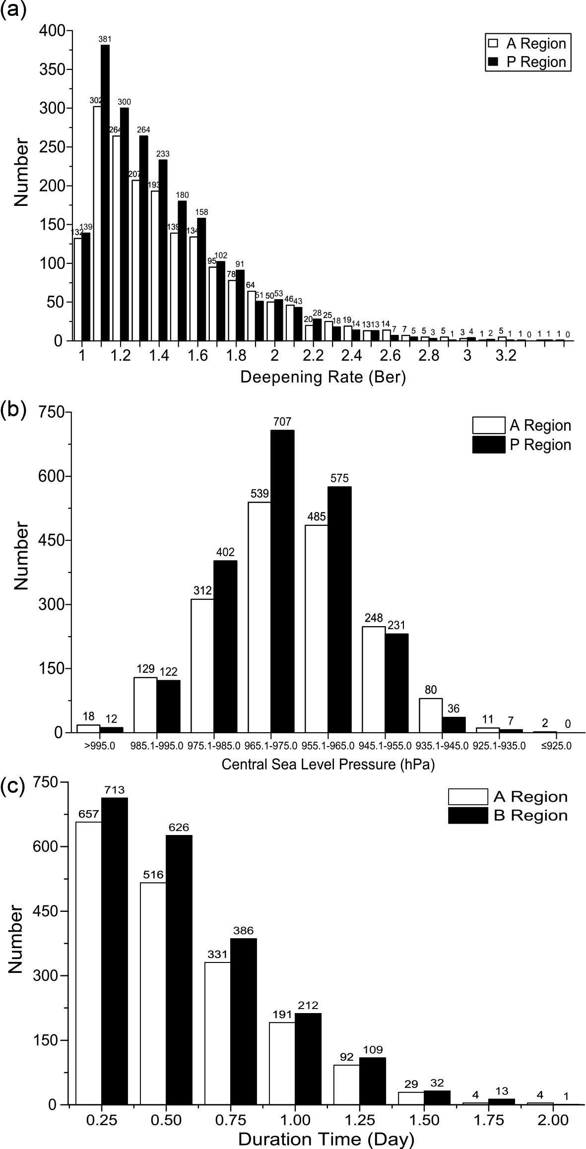 Figure4. Histogram of numbers of ECs over the A region and P region from 1979 to 2016: (a) ECs with their maximum-deepening-rates of central SLP; (b) ECs with their minimum central SLP; (c) ECs with their DTDs.
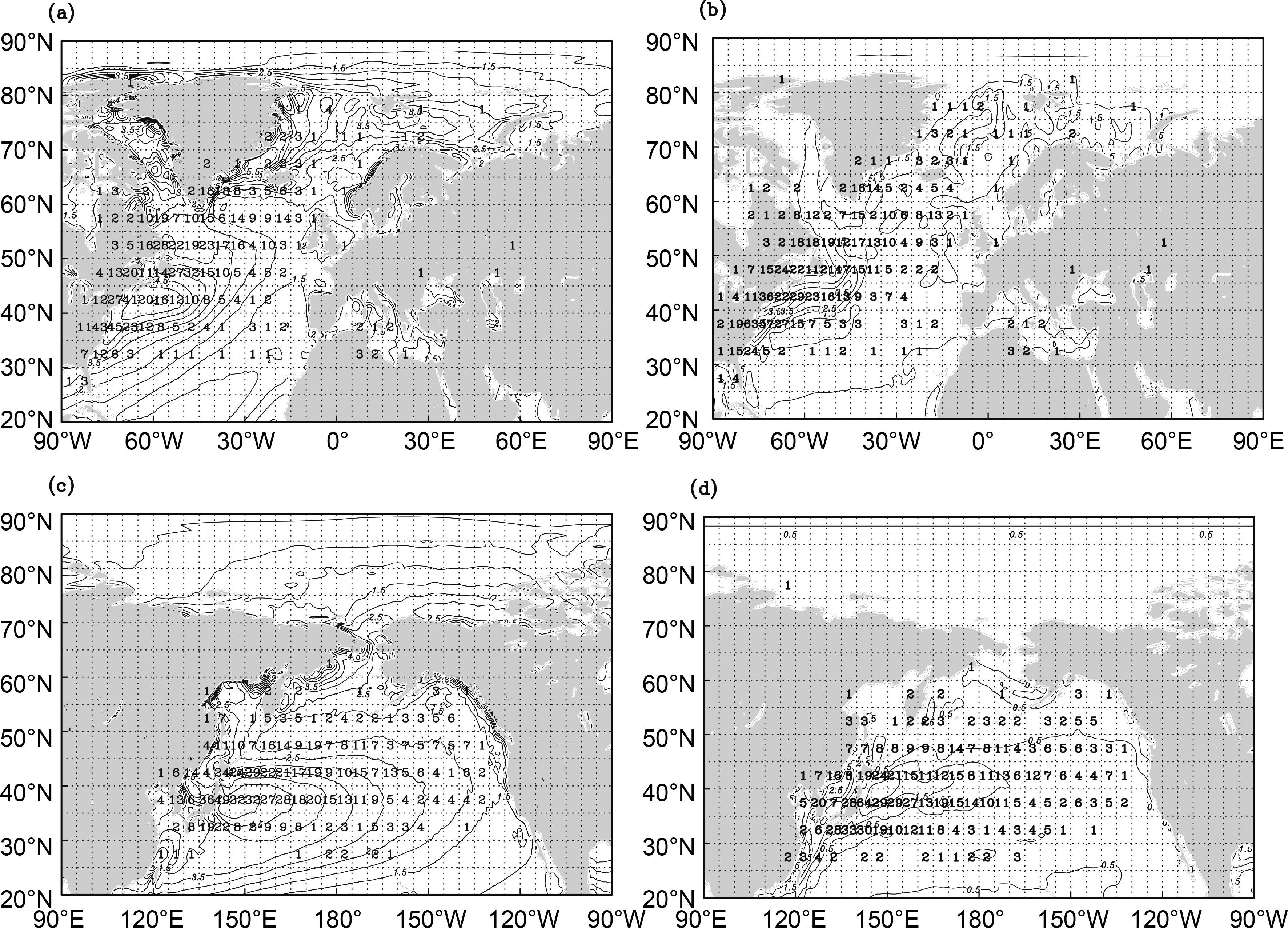 Figure6. As in Fig. 2 but for the winter season from 1979/80 to 2015/16.
For ECs over the northern Atlantic, their spatial distribution extends northeastward along the east coast of North America (Sanders and Gyakum, 1980; Wang and Rogers, 2001; Allen et al., 2010). There are three frequent-occurrence areas of ECs: the area along the coast of North America (from 70°W to 55°W); the area from 50°W to 40°W; and the area from 30°W to 25°W (Wang and Rogers, 2001). The EC distribution revealed by Allen et al. (2010) over the northern Atlantic was different to that revealed by Wang and Rogers (2001), showing only two distinct frequent-occurrence areas of ECs over the northern Atlantic—from 75°W to 50°W and from 50°W to 30°W.
Several observational or modeling studies have revealed that the large-scale environmental backgrounds, such as the atmospheric and oceanic circulations, have significant influences on the spatial distribution of ECs (Konrad II and Colucci, 1988; Kelly et al., 1994; Lackmann et al., 1996; Yoshida and Asuma, 2004; Black and Pezza, 2013; Zhang et al., 2017). Several factors are thought to be responsible for the genesis and development of ECs, including baroclinic instability (Sanders and Gyakum, 1980; Bosart, 1981; Anthes et al., 1983; Roebber, 1984; Reed and Albright, 1986; Nuss and Anthes, 1987; Rogers and Bosart, 1991; Iwao et al., 2012), thermal forcing (Anthes and Keyser, 1979; Chen et al., 1983; Gyakum, 1983a,b; Chen and Dell’osso, 1987; Liou and Elsberry, 1987; Kuo et al., 1991; Dal Piva et al., 2011; Fink et al., 2012; Hirata et al., 2015), advection of vorticity and temperature (Petterssen and Smebye, 1971; Bosart and Lin, 1984; Sanders, 1986; Lupo et al., 1992; Rausch and Smith, 1996; Strahl and Smith, 2001; Yoshida and Asuma, 2004), potential vorticity and tropopause folding (Bosart and Lin, 1984; Uccellini et al., 1985; Whitaker et al., 1988; Zehnder and Keyser, 1991; Browning and Golding, 1995; Cordeira and Bosart, 2011; Binder et al., 2016), upper-level jet streams (Uccellini and Johnson, 1979; Uccellini et al., 1984; Ruscher and Condo, 1996; Yoshida and Asuma, 2004; Rivière et al., 2010), and the combination of multiple factors (Bullock and Gyakum, 1993; Nesterov, 2010). Furthermore, there are also other factors that may affect ECs, such as topographic effects (Kristjánsson et al., 2009), the northern Atlantic Oscillation (NAO, Nesterov, 2010), and the horizontal resolution of data (Kouroutzoglou et al., 2011).
Although the climatological features of ECs over the Pacific and Atlantic have been investigated in several studies (Sanders and Gyakum, 1980; Roebber, 1984; Sanders, 1986; Gyakum, et al. 1989; Chen et al., 1992; Wang and Rogers, 2001; Zhang et al., 2017), to the best of our knowledge there have been no EC studies that have examined two basins in the Northern Hemisphere using single detection criteria. In this paper, the characteristics of ECs over the Northern Hemisphere from January 1979 to December 2016 are investigated. The classical definition of an EC is modified considering not only the rapid drop of the central SLP of the cyclone, but also the strong wind speed at the height of 10 m in which the maximum wind speeds greater than 17.2 m s?1 are included. The overall aim is to reveal the climatological features of ECs over two basins in the Northern Hemisphere.
The rest of the paper is structured as follows: Section 2 introduces the data and methods. The modification of the EC definition is discussed in section 3. Section 4 presents the climatological features of ECs, such as their spatial distribution, intensity, seasonal variation, interannual variation, and moving tracks. Finally, concluding remarks are given in section 5.
2.1. Data
The data utilized in the present study are as follows:(1) ERA-Interim data (
(2) OISST data (
2
2.2. Methods
A revised cyclone detection and tracking algorithm, initially developed by Hart (2003), is used to identify and track the extratropical cyclones over the Northern Hemisphere from January 1979 to December 2016. Some additional restriction conditions are added in order to eliminate tropical cyclones, as well as extratropical cyclones whose life cycles are shorter than 24 hours. The specific methods are as follows: (1) the minimum SLP within any 5°×5° domain should be smaller than 1020 hPa, and the location of the minimum SLP should not be at the border of this 5°×5° domain; (2) the life cycle of the extratropical cyclone should be longer than 24 hours; (3) the change of SLP within a 5°×5° domain should be equal to or less than 2 hPa; and (4) the topographic elevation should be below 1500 m in order to eliminate the interference of plateau thermal low-pressure systems.For the tracking algorithm of cyclone, the method put forward by Hart (2003) is also used. Assuming that there exists one cyclone (A) at t?δt and one cyclone (B) at t, where the distance between A and B is δd, the restriction conditions for tracking the cyclone are as follows: (1) δt should be shorter than 24 hours; (2) cyclone B at t is the closest one to cyclone A at t?δt; (3) the moving speed of cyclone A to cyclone B (δd/δt) should be less than 45 m s?1; (4) δd<δdmax [where δdmax is the maximum moving distance within the period δt, and δdmax = max (500 km, 3×δt×Vprev), in which Vprev is the moving speed of cyclone A during the period from t?2δt to t?δt]; and (5) the change in cyclone moving direction from period t?2δt to t?δt to the period t to t?δt should be limited within a certain range.
3.1. Modification of EC definition
The original definition of an EC initially quantified by Sanders and Gyakum (1980) emphasized the rapid central-pressure-drop of the cyclone. However, the factor of wind speed has not yet been considered in the definition of an EC. In this subsection, we discuss the significance of wind speed in defining an EC.In order to understand the definition of an EC deeply and clearly, it is useful to review famous ECs, such as the QE-II cyclone of 10?11 September 1978 (Gyakum, 1983a,b; Uccellini, 1986; Gyakum, 1991) and the Presidents’ Day cyclone of 18?19 February 1979 (Bosart, 1981; Bosart and Lin, 1984; Uccellini et al., 1984, 1985; Whitaker et al., 1988). The QE-II cyclone experienced an extraordinarily rapid 24-hour central pressure fall of nearly 60 hPa. Based upon extensive investigations of these cyclones, it can be summarized that common and widely accepted features of ECs are: (1) a rapid drop of central pressure; (2) fast cyclogenesis; (3) strong winds; and (4) heavy rain-/snowfall. Usually, these features are integrated, and cannot be isolated. Among these four features, strong wind associated with explosive deepening is the most dominant factor that may cause severe damage, just like a tropical cyclone.
For tropical cyclones, the Typhoon Committee of the World Meteorological Organization (WMO) (
Yoshida and Asuma (2004) calculated the deepening rate of cyclone SLP(RSLP) in the following way:
where p is the SLP of the cyclone center, t is the analysis time in hours, and

Applying ERA-Interim data into Eq. (1), all extratropical cyclones whose deepening rates are greater than or equal to 1 Bergeron are selected. It is found that, over the entire Northern Hemisphere (20°?90°N), there are a total of 6392 ECs from January 1979 to December 2016.
In order to examine the wind speeds in the EC definition, the ERA-Interim wind speeds associated with extratropical cyclones at the height of 10 m are analyzed carefully. It is found that, for some extratropical cyclones, although their deepening rates of central SLP are greater than 1 Bergeron, their winds are sometimes very weak, and their maximum wind speeds can even be near to 8.2 m s?1. As the major threat of ECs over oceans to shipping safety is due to strong winds, and the WMO suggests that gales over oceans greater than Force 8 on the Beaufort scale (17.2 m s?1) should constitute a gale warning, it is thus reasonable and acceptable to choose a wind speed of 17.2 m s?1 as the threshold value in the modified definition of an EC. In total, 1112 extratropical cyclones whose maximum wind speeds are less than 17.2 m s?1 are eliminated.
Figure 1 shows the geographic map of the Northern Hemisphere. According to the geographic locations of the Atlantic and the Pacific, the Northern Hemisphere is separated into two regions—the “A region” (20°?90°N, 90°W?90°E) and “P region” (20°?90°N, 90°E?90°W)—with the same spatial size (see Fig. 1). With this division, the entire Northern Hemisphere is completely covered by these two regions. In addition, the northern Atlantic region (20°?80°N, 90°W?20°E) and northern Pacific region (20°?80°N, 100°E?100°W) are also defined.
In previous studies (Roebber,1984; Gyakum et al., 1989; Zhang et al., 2017), the latitude of 60°N in the EC definition has been modified by the mean latitude of most EC locations. Roebber (1984) adjusted 60°N to 42.5°N—the approximate latitude of maximum EC occurrence over the Northern Hemisphere. Similarly, Gyakum et al. (1989) and Zhang et al. (2017) adjusted 60°N to 45°N—a region slightly to the north where most ECs occurred over the northern Pacific. In the present study, the mean latitudes of ECs over the A region and P region are 49.53°N and 43.21°N, respectively. For convenience, the mean latitudes in the EC definition are adjusted geostrophically to 50°N over the A region and 45°N over the P region. Subsequently, there are a total of 3916 ECs over the Northern Hemisphere.
Thus, in the present study, an EC is newly defined as a surface low-pressure system whose deepening rate of central SLP falls at least 1 Bergeron within 12 hours and lives longer than 24 hours with a maximum wind speed at the height of 10 m greater than 17.2 m s?1. The deepening rate of an EC is calculated as follows:
where

2
3.2. Some specific terms related to ECs
In order to elucidate concisely, nine specific terms related to ECs are listed in Table 1. Moreover, the baroclinic index (BI) at 850 hPa used by Iwao et al. (2012) is employed to denote the lower-level atmospheric baroclinicity. The formula is as follows:| No. | Abbreviation | Definition | Detailed description |
| 1 | IDM | Initial explosive-deepening moment | The first moment when the deepening rate of an EC is greater than or equal to 1 Bergeron. |
| 2 | MDM | Maximum deepening-rate moment | The moment when the deepening rate of an EC reaches its maximum value. |
| 3 | LDM | Last explosive-deepening moment | The last moment when the deepening rate of an EC is greater than or equal to 1 Bergeron. |
| 4 | DTD | Duration time of explosive-deepening | The duration time of an EC from IDM to LDM, or the period of an EC whose deepening rate of central SLP is greater than or equal to 1 Bergeron. |
| 5 | RAC | Rapid-deepening area of an EC | The area where ECs are concentrated at MDM. |
| 6 | OAC | Origin area of initial explosive-deepening of cyclone | The area where ECs are concentrated at IDM. |
| 7 | PRET | Pre-explosive-developing track | The track of an EC from generation to IDM. |
| 8 | EXT | Explosive-developing track | The track of an EC from IDM to LDM. |
| 9 | POET | Post-explosive-developing track | The track of an EC from LDM to its death. |
Table1. Nine specific terms related to ECs.
where f is the Coriolis parameter,


4.1. Annual climatology of ECs
34.1.1. Features of spatial distribution
Figure 2 shows the spatial distribution of ECs over the A region and P region from 1979 to 2016. According to previous studies, ECs tend to occur over regions with a larger SST gradient or stronger lower-level atmospheric baroclinicity. Over the western boundaries of the Atlantic and the Pacific, influenced by warm and cold oceanic currents, there are large SST gradients and strong atmospheric baroclinicity, which are beneficial to EC occurrence. Most ECs are located near the east coast of the A region, and the east of Japan in the P region. Over the northeast of the ocean, the SST gradient/atmospheric baroclinicity is smaller/weaker than that over the southwest of the ocean, but there are also many ECs. Previous studies indicate that upper-level forcing is more dominant over that area. The spatial distributions of ECs over these two regions are in a northeast?southwest direction, but the distribution of ECs over the A region tends to extend northward. In addition, the spatial distributions of OAC (see Table 1 for definition) over these two regions (Figs. 2b and d) are located southwestward compared with RAC (see Table 1 for definition) (Figs. 2a and c). Meanwhile, different from previous statistics on the distribution of ECs over the Northern Hemisphere, we find that ECs may occur over the Arctic region, land, and some intercontinental seas as well. Figure2. Geographic distributions of the number of ECs within 5°×5° bins over two basins in the Northern Hemisphere from 1979 to 2016. RAC distributions of ECs over the A region and P region are shown in (a) and (c), respectively. OAC distributions of ECs over the A region and P region are shown in (b) and (d), respectively. Contours in (a) and (c) represent the BI at 850 hPa, calculated by Eq. (3) (units: 1×10?7 m K?1 s?2). Contours in (b) and (d) represent the SST gradient (units:1×10?5 K m?1).
Figure 3 shows the mean atmospheric circulation of the Northern Hemisphere from 1979 to 2016. It is found that, at 500 hPa (Fig. 3a), the spatial distributions of ECs over the A and P regions are in the east of troughs. The amplitude of the North America trough is larger than that of the East Asia trough, and thus the northward distribution of ECs over the A region is more obvious than that over the P region. At 200 hPa (Fig. 3b), the effect of upper-level jet streams (≥30 m s?1) over the P region is more obvious than that over the A region.
3
4.1.2. Features of EC intensity
The numbers of ECs along with their maximum deepening rates of central SLP over the A and P regions are shown in Fig. 4a. It is seen that, starting from 1.1 Bergeron, the number of ECs decreases rapidly as the deepening rate increases. The mean latitudes in the definition of ECs over the A region (50°N) and P region (45°N) are different. In order to compare the deepening rates of ECs over these two regions, the mean latitude in the definition of ECs over the P region is adjusted geostrophically to 50°N. The results show that, over the A region and P region, the mean deepening rate of ECs is 1.46 and 1.53 Bergeron, respectively (see Table 2). In addition, the maximum value over these two regions is 3.47 and 3.63 Bergeron, respectively, suggesting that ECs over the P region may deepen slightly faster than ECs over the A region on average.| Season | Maximum deepening rate (Bergeron) | Minimum central SLP (hPa) | DTD (days) | |||||
| A region | P region | A region | P region | A region | P region | |||
| Winter | 1.52 | 1.45(1.57) | 964.1 | 966.6 | 0.60 | 0.59 | ||
| Spring | 1.37 | 1.40(1.51) | 971.3 | 970.2 | 0.51 | 0.59 | ||
| Summer | 1.26 | 1.25(1.35) | 976.3 | 972.7 | 0.44 | 0.4 | ||
| Autumn | 1.39 | 1.39(1.50) | 966.6 | 967.3 | 0.54 | 0.55 | ||
| Total | 1.46 | 1.42(1.53) | 966.5 | 967.8 | 0.567 | 0.574 | ||
Table2. Comparison of ECs over the A region and P region in the four seasons. Bold numbers within brackets are the maximum deepening rate of central SLP over the P region when the mean latitude of 50°N is used in the definition of an EC.
Figure 4b shows the numbers of ECs along with their minimum central SLP over the two regions. Over both the A region and P region, the number of ECs within 965.1?975.0 hPa is the maximum, followed by the number of ECs within 955.1?965.0 hPa, 975.1?985.0 hPa, 945.1?955.0 hPa, 985.1?995.0 hPa, 935.1?945.0 hPa, >995.0 hPa, 925.1?935.0 hPa, and finally <925.0 hPa. Over the A region, the number of ECs within 955.1?985.0 hPa is less than that over the P region. In other ranges, the number of ECs over the P region is more. Over the P region, there are fewer extreme ECs (strong or weak). In contrast, over the A region, there are more extreme ECs (strong or weak). Over the A region, the mean SLP and the minimum SLP are 966.5 hPa and 913.1 hPa, respectively. Similarly, over the P region, the mean SLP and the minimum SLP are 967.8 hPa and 925.4 hPa, respectively. Over the A region, the mean SLP and the minimum SLP are smaller, suggesting that the mean intensity of ECs over the A region is stronger than that over the P region.
Over the A and P regions, the numbers of ECs with their DTDs (see Table 1 for definition) are shown in Fig. 4c. For ECs over these two basins in the Northern Hemisphere, the DTD of cyclones is no longer than 2.00 days, and the number of ECs decreases with the increase in DTD. Except for ECs with DTDs of 2.00 days, the number of ECs over the A region with other DTDs is less than that over the P region. In addition, within the range of 0.50?2.00 days, the difference in the number of ECs between the A and P regions gradually decreases. The mean DTD of ECs over the A region (0.567 days) is shorter than that over the P region (0.574 days). For ECs with DTDs of 2.00 days, there are only five ECs from1979 to 2016, and four of them occur over the A region. This suggests that, although the mean DTD of ECs over the A region is shorter than that over the P region, there are more extreme ECs (DTD of 2.00 days).
2
4.2. Seasonal climatology of ECs
Figure 5 shows the monthly frequency distribution of ECs over the A and P regions. The numbers of ECs over these two regions peak in January, and for both their minimum appears in July. Over the A region, however, there are more ECs in February and December. Over the P region, there are more ECs in March and November.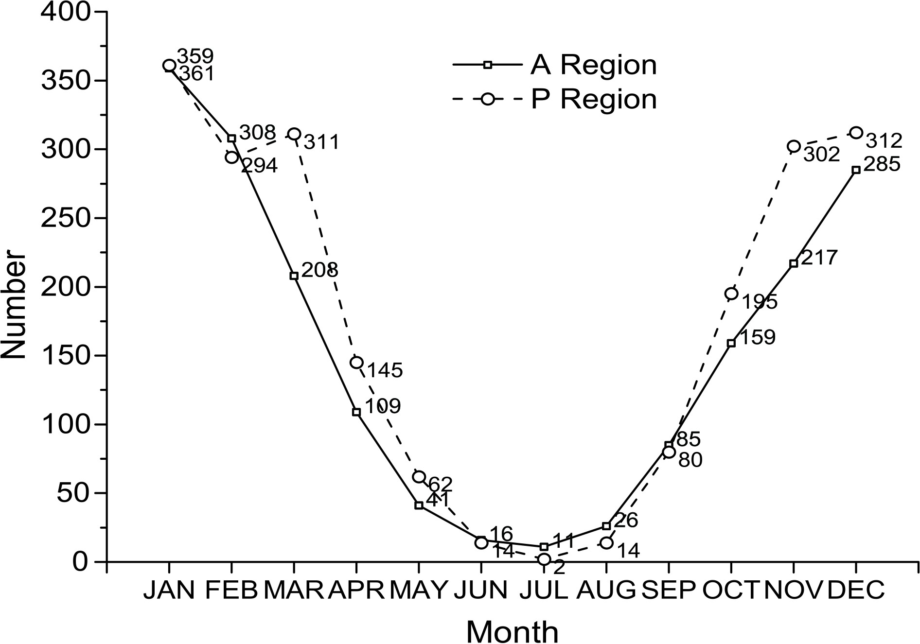 Figure5. Monthly occurrence frequencies of ECs over the A region and P region from 1979 to 2016.
Due to the obvious difference in the monthly frequencies of ECs between the A and P regions, the seasonal climatology of ECs is investigated. It is shown that the number of ECs over the two regions is at a maximum in the winter season (from December to February), followed by autumn (from September to November), spring (from March to May) and summer (from June to August).
3
4.2.1. Winter season
In the winter season, the difference in the number of ECs between the A and P regions is at a minimum. There are 927 ECs over the A region and 939 ECs over the P region. The spatial distribution (Fig. 6) of ECs over the two regions is southwestward?northeastward. Over the A region (Figs. 6a and b), more ECs are concentrated near the east coast of North America and Newfoundland. Different from the spatial distribution of ECs from 1979 to 2016, there is a new frequent-occurrence center of RAC over the eastern coast, and the frequent-occurrence center of OAC over the east coast is the most prominent. Over the P region (Figs. 6c and d), more ECs occur over the ocean to the east of Japan. Compared with the spatial distribution of ECs from 1979 to 2016, there are no obvious frequent-occurrence centers of ECs at both MDMs and IDMs (see Table 1 for definitions) over the northeastern Pacific. Meanwhile, most ECs over the Korean Peninsula and Japan Sea occur in winter. In the winter season, over the northwestern Atlantic, the lower-level atmospheric BI reaches 6×10?7 m K?1 s?2 and the SST gradient reaches 4.5×10?5 K m?1. Similarly, over the northwestern Pacific, the BI and SST gradient reach 5.5×10?7 m K?1 s?2 and 2.5×10?5 K m?1, respectively. Over the A region, both the BI and SST gradient are stronger and larger than those over the P region. This is perhaps the reason leading the increase in the number of ECs over the A region in the winter season.During the winter season, the large-scale atmospheric circulation changes. At 500 hPa (Fig. 7a), the amplitudes of troughs increase obviously, which may provide a favorable background for the development of ECs. Meanwhile, the wind speed at 200 hPa also increases (Fig. 7b). The obvious upper-level jet streams over the A and P regions are favorable factors for EC development.
 Figure7. As in Fig. 3 but for the winter season from 1979/80 to 2015/16.
3
4.2.2. Spring season
Spring is the season with the maximum difference in the number of ECs between the A and P regions. There are 358 ECs over the A region and 518 ECs over the P region. In terms of spatial distribution (Fig. 8), over the A region, the frequent-occurrence centers of RAC over the ocean in the east and the north of Newfoundland are more obvious. However, the distribution of OAC is different, with most ECs occurring over the land along the east coast. Except for the frequent-occurrence centers of the ocean in the east of Japan, many ECs also occur over the central and northeastern Pacific. Compared with the winter season, both the BI and SST gradient over the A and P regions are weaker and smaller. This is one of the important factors why the number of ECs in the spring season is less than that in the winter season. During the spring season, the BI over the P region (3.5×10?7 m K?1s?2) is slightly stronger than that over the A region (3×10?7 m K?1s?2), which is perhaps one of the reasons why there are more ECs over the P region. Figure8. As in Fig. 2 but for the spring season from 1979 to 2016.
Different from the winter season, the amplitudes of troughs at 500 hPa decrease in the spring season (Fig. 9a). At 200 hPa (Fig. 9b), the wind speeds drop sharply, and only the upper-level jet stream over the P region is obvious. The aforementioned changes of atmospheric circulation maybe a crucial reason why the number of ECs in the spring season is less than that in the winter season, especially over the A region.
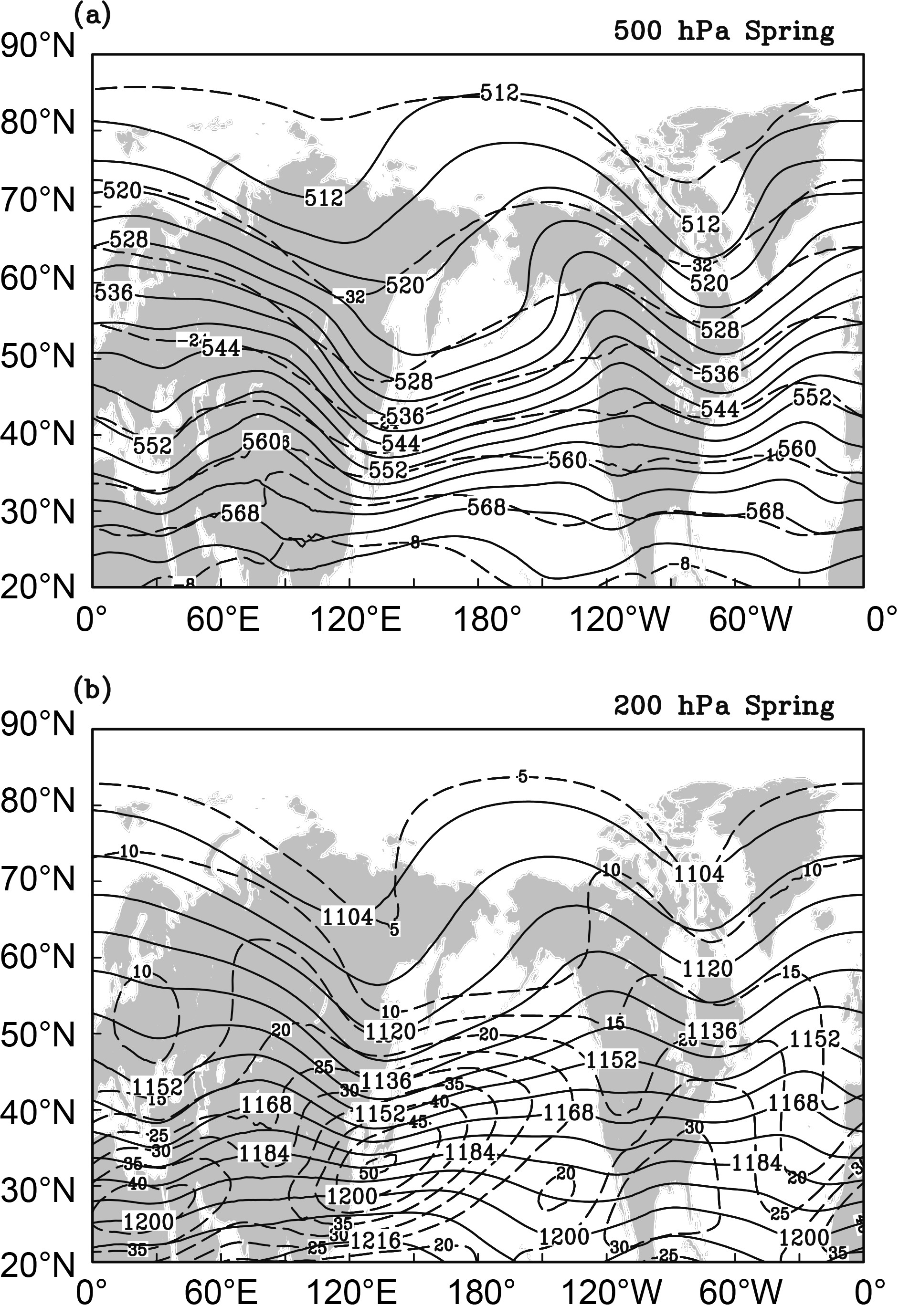 Figure9. As in Fig. 3 but for the spring season from 1979 to 2016
3
4.2.3. Summer season
Summer is the season when the number of ECs is at a minimum. There are only 53 ECs over the A region and 30 over the P region. The spatial distribution of ECs is more scattered. Over the A region (Figs. 10a and b), the spatial distributions of RAC and OAC are concentrated over the area (40°?60°N, 75°?20°W). However, over the P region (Figs. 10c and d), the spatial distribution of ECs bounded by 175°E can be divided into two parts. Lower-level atmospheric baroclinicity in summer is the weakest in all four seasons, and the SST gradient is the smallest. In addition, for the mean circulations at 500 hPa and 200 hPa (Fig. 11), the amplitudes of troughs or ridges are small and the wind speeds are weak. All of the above changes in atmospheric and oceanic environments are not conducive to the development of ECs. Therefore, there are few ECs over the two basins in the Northern Hemisphere in the summer season. Figure10. As in Fig. 2 but for the summer season from 1979 to 2016.
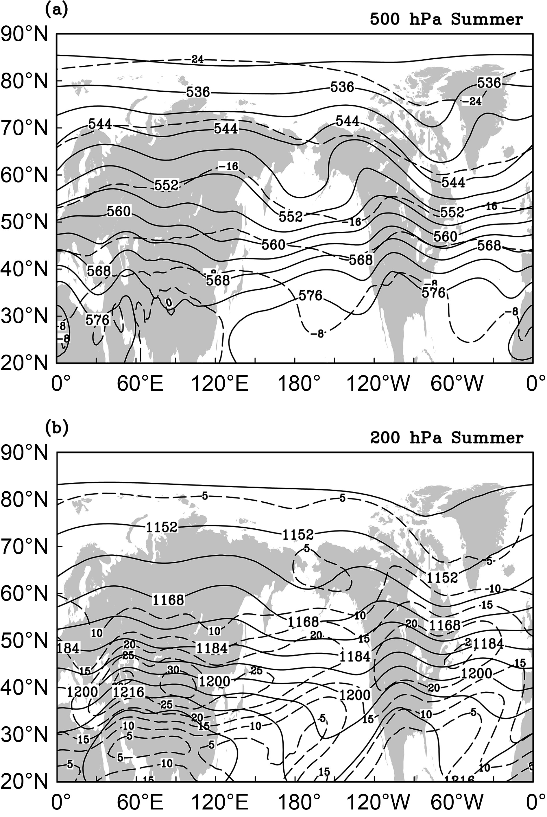 Figure11. As in Fig. 3 but for the summer season from 1979 to 2016.
3
4.2.4. Autumn season
During the autumn season, there are 461 ECs over the A region and 577 ECs over the P region. Over the A region (Figs. 12a and b), the spatial distributions of RAC and OAC show similar patterns to those in the spring season. Most ECs at their MDMs are located over the ocean in the east of Newfoundland and the land in the north of Newfoundland. At IDMs, there are two obvious frequent-occurrence centers: one is over land along the east coast, and the other is over the ocean to the east of Newfoundland. However, in terms of the spatial distributions of RAC and OAC over the P region (Figs. 12c and d), their distributions are significantly different from those in spring season. To the north of 45°N, there are three frequent-occurrence centers over the northwestern Pacific. Besides, the frequent-occurrence center of ECs over the northeastern Pacific is the most significant in all four seasons. Over the western part of oceans, the SST gradient is not much different, but the BI over the P region (4×10?7 m K?1 s?2) is stronger than that over the A region (3×10?7 m K?1 s?2). Figure12. As in Fig. 2 but for the autumn season from 1979 to 2016.
Regarding the mean upper-level circulations (Fig. 13), the spatial distribution over the A region in autumn is similar to that in the spring season. Most ECs are concentrated in the east of the North America trough at 500 hPa, and the upper-level jet stream at 200 hPa is not obvious. Over the P region, however, there is a marked change in atmospheric circulation in the autumn season. Perhaps affected by the southward extension of the subtropical high, a new trough forms to the east of the East Asia trough. This maybe an important reason why the EC distribution over the P region in the autumn season (Figs. 12c and d) is different from that in other seasons. At 200 hPa, there is an upper-level jet stream over the P region, but the jet stream axis in the autumn season is located farther north than that in the spring season.
 Figure13. As in Fig. 3 but for the autumn season from 1979 to 2016.
Table 2 lists the characteristics of ECs over the A and P regions in the four seasons (note: the deepening rate of ECs over the P region is adjusted geostrophically to 50°N). It is found that, on average, ECs over the P region usually deepen faster than those over the A region in the four seasons. The minimum central SLP of ECs over the A region in winter is 964.1 hPa, and in autumn it is 966.6 hPa. In spring, however, it is 970.2 hPa, and in summer it is 972.7 hPa. Over the A region, the DTD of ECs in winter is 0.60 days, and in summer it is 0.44 days. Over the P region, however, the DTD of ECs in spring is 0.59 days, and in autumn it is 0.55 days.
2
4.3. Features of interannual variation
Figure 14a shows the time series of the annual number of ECs over the A and P regions. The mean annual number of ECs over the A region and P region is 48.00 and 55.05, respectively. Except for 1985, 1989, 1995, 2002, 2013 and 2015, the number of ECs over the P region is more than that over the A region. In terms of standard deviation, the value over the P region (5.85) is smaller than that over the A region (6.78), suggesting that the interannual variation of ECs over the P region is smoother. Figure 14b-e shows the interannual variations of the number of ECs in the four seasons. In the winter season (Fig. 14b), there are 14 years in which the number of ECs over the A region is more than that over the P region, whereas there are 17 years in which the number of ECs over the P region is more. In addition, there are 6 years in which number of ECs over the two regions are the same. For the mean annual number of ECs, there are 25.05 ECs over the A region and 25.38 ECs over the P region per year. The standard deviation of the number of ECs over the A region and P region is 3.73 and 4.41, respectively. This suggests that, different from the entire period, the interannual variation of ECs over the A region is smoother in winter.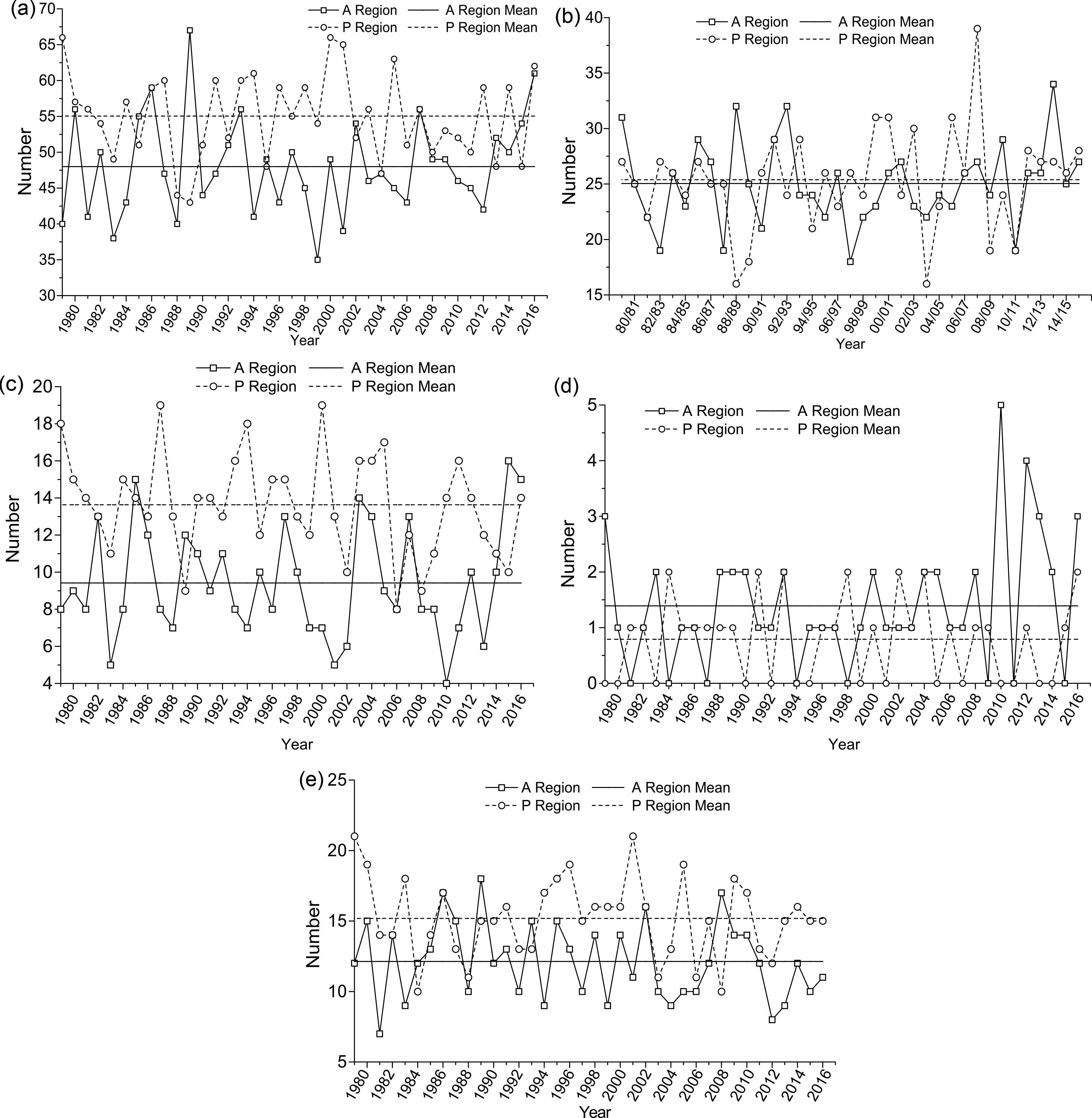 Figure14. Interannual variations of ECs over the A region (solid lines) and P region (dashed lines) from 1979 to 2016: (a) the whole time series; (b) winter; (c) spring; (d) summer; (e) autumn.
During the spring season (Fig. 14c), there are only 5 years (1985, 1989, 2007, 2015 and 2016) in which the number of ECs over the A region is more than that over the P region. The difference in EC annual numbers over the A and P regions is large. The mean annual number of ECs over the A and P regions is 9.42 and 13.63, respectively. However, the difference in the standard deviation of the number of ECs over two regions is small, and their values over the A region and P region are 2.98 and 2.68, suggesting that the interannual variations of ECs over the two regions are similar.
During the summer season (Fig. 14d), over the A region, there are 8 years in which there is no EC occurrence, and the year with the most ECs (five) is 2010, followed by 2012 (four). For the number of ECs over the A region, the average is 1.39 and the standard deviation is 1.14. Over the P region, there are 15 years in which there is no EC occurrence, and the annual number of ECs is no more than two. The average and standard deviation of the number of ECs over the P region are 0.79 and 0.73, respectively.
In the autumn season (Fig. 14e), the numbers of ECs over the A region in 1984, 1987, 1989, 1993 and 2008 are more than those over the P region. Meanwhile, the numbers of ECs over the A and P regions in 1982, 1986 and 2002 are the same. In the remaining years, there are more ECs over the P region. The annual number of ECs over the A region and P region is 12.13 and 15.18, respectively. In addition, the standard deviation of the number of ECs over the A region and P region is 2.70 and 2.78, respectively. The difference in the standard deviation over the A and P regions is at a minimum, suggesting that the interannual variation of ECs during autumn is similar in the four seasons.
2
4.4. Features of moving tracks
Regarding the moving tracks of ECs over the Northern Hemisphere, we investigate those ECs with maximum deepening rates greater than or equal to 2 Bergeron. According to the spatial distribution of EC moving tracks over the northern Atlantic (Fig. 15a), ECs can be classified into two types (Fig. 16): those moving north-northeastward near the mainland (named A-NNE-type ECs), and those moving northeastward from the east coast (named A-NE-type ECs). The A-NE-type ECs are especially dominant over the A region. Similarly, ECs over the northern Pacific (Fig. 15b) can be classified into three types (Fig. 16): those moving northeastward from offshore East Asia (named P-NE-type ECs); those moving east-northeastward from the ocean to the east of Japan (named P-ENE-type ECs); and those moving north-northeastward over the northeastern Pacific (named P-NNE-type ECs). P-ENE-type ECs are dominant over the P region.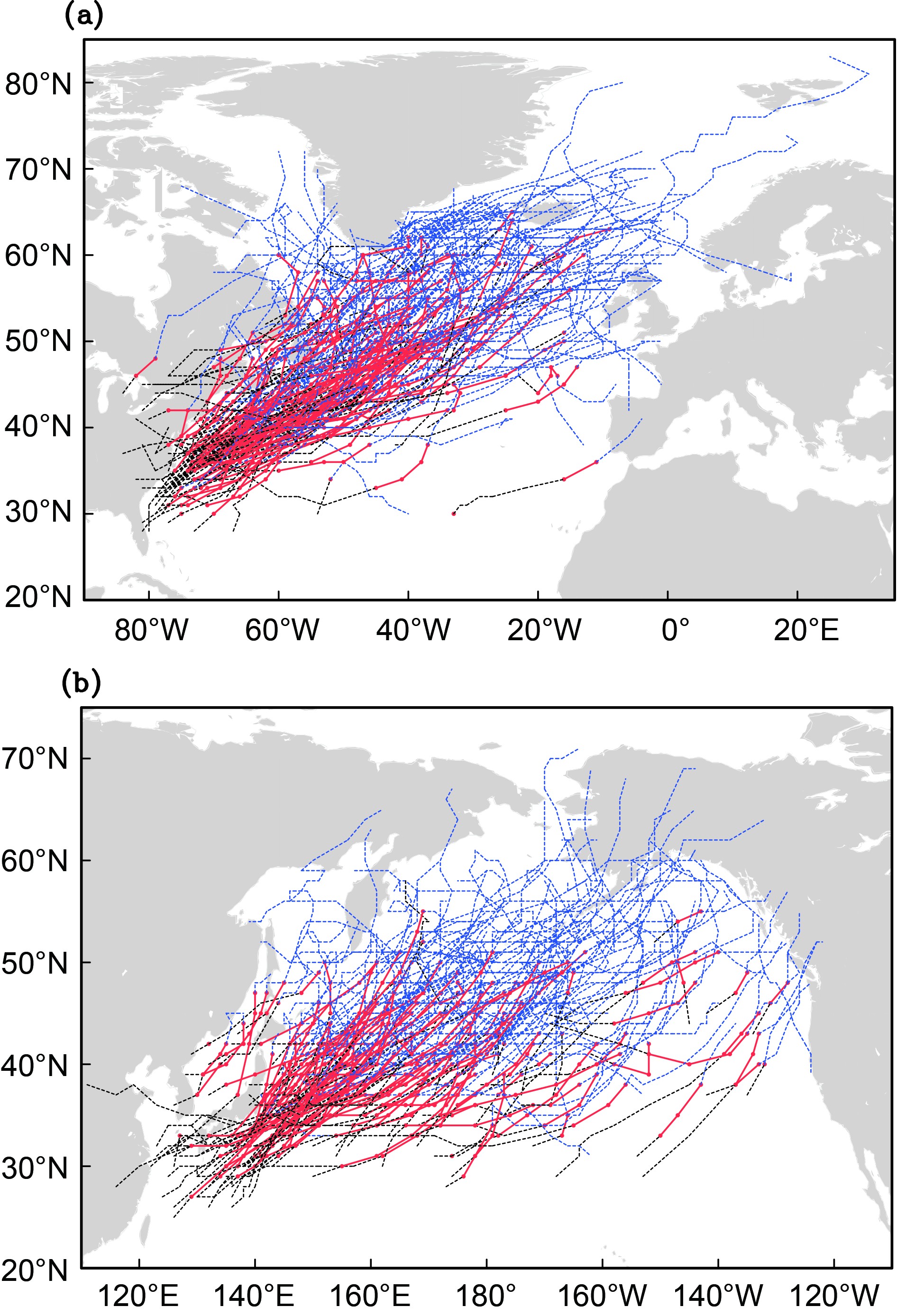 Figure15. Moving tracks of ECs with their maximum deepening rates greater than or equal to 2 Bergeron from 1979 to 2016: (a) over the northern Atlantic; (b) over the northern Pacific. Black lines, red lines and blue lines represent PRET, EXT and POET (see Table 1 for definitions), respectively.
 Figure16. Schematic diagram of moving tracks of ECs over two basins in the Northern Hemisphere.
From May to September, the general characteristics of EC moving tracks are as follows: the number of ECs with poleward tracks is reduced with the decrease in ECs. However, from October to April, as the number of ECs firstly increases and then decreases, the number of ECs with poleward tracks grows. It is worth noting that there are ECs with poleward tracks in every month over the northeastern Pacific. Over the A region, in order to compare the years with more ECs (1980, 1985, 1986, 1989, 1993, 2002, 2007, 2015 and 2016) and the years with fewer ECs (1979, 1981, 1983, 1988, 1994, 1999, 2001, 2006 and 2012), we take 1989 (more ECs, Fig. 17b) and 1983 (fewer ECs, Fig. 17a) as examples. It is found that the number of ECs in the year with fewer A-NNE-type ECs is relatively less. Similarly, over the P region, in order to compare the years with more ECs (1979, 1986, 1987, 1991, 1993, 1994, 1996, 1998, 2000, 2001, 2005 and 2016) and the year with fewer ECs (1983, 1985, 1988, 1989, 1995, 2004, 2008, 2011, 2013 and 2015), we take 2016 (more ECs, Fig. 17c), 1983 (fewer ECs, Fig.17a) and 1989 (fewer ECs, Fig. 17b) as examples. It is found that the number of ECs in the year with more P-NE or P-NNE type ECs is relatively high. Except for 2015 (not shown), the number of P-NE type or P-NNE type ECs is relatively lower during the year with few ECs.
 Figure17. Moving tracks of ECs over two basins in Northern Hemisphere: (a) in 1983, (b) in 1989, (c) in 2016.
It should be pointed out that various researchers have used different EC definitions. For example, Sanders and Gyakum (1980), when studying ECs in the Northern Hemisphere, used 60°N as the adjusting latitude in the definition of an EC. Wang and Rogers (2001) and Yoshida and Asuma (2004) used 60°N as the adjusting latitude when examining ECs over different sectors of the northern Atlantic and Northwest Pacific, respectively. Zhang et al. (2017) modified the definition of an EC given by Sanders and Gyakum (1980) as a cyclone whose central SLP decline normalized at 45°N is greater than 12 hPa within 12 hours. However, in the present study, we consider the difference in the mean latitude of most EC occurrence locations over the Atlantic basin (50°N) and Pacific basin (45°N), which suggests that the current EC definition in each basin may reflect their specific local nature.
The OAC and RAC over the northern Atlantic and northern Pacific are a focus. Both are in southwest?northeast directions, but the distribution of ECs tends to extend northward over the A region.
Over the A region, the deepening rate of ECs is smaller than that over the P region. Also, the DTD of ECs is shorter, but their intensity is stronger. During the winter, spring and autumn seasons, there is an obvious frequent-occurrence area of ECs over the east coast. A stronger lower-level atmospheric baroclinicity and North America trough at 500 hPa provide favorable backgrounds for ECs. The effect of 200-hPa jet streams is more prominent in the winter season.
Over the P region, the deepening rate of ECs is greater, and the DTD of ECs is longer, but their intensity is weaker. The region to the east of Japan is an obvious frequent-occurrence area of ECs. During the spring and autumn seasons, more ECs occur over the northeastern Pacific. Lower-level atmospheric baroclinicity provides a favorable environment for ECs. Except in the summer season, the distribution of the upper-level jet stream is a favorable background condition for ECs.
According to the geographic distribution of EC moving tracks over the A region, ECs can be classified into two types: A-NNE-and A-NE-type ECs. Over the P region, ECs can be classified into three types: P-NE-, P-ENE- and P-NNE-type ECs. Basically, all moving tracks are in southwest?northeast directions, but NNE-type ECs over the A and P regions tend to move northward.
The number of ECs exhibits an obvious periodic variation, but the reason is unclear. Nesterov (2010) pointed out that ECs are affected by the NAO. Taking the A region as an example, we analyzed the relationship between the number of ECs and the NAO (not shown).It was found that, in some years, EC occurrence bears a good correspondence with the NAO, but there is no statistically significant (95% confidence level) relationship in other years. It seems that a complicated relationship exists between the number of ECs and the NAO, which needs to be further explored.
Acknowledgements. All authors express their thanks to the National Natural Science Foundation of China for financial support (Grant Nos. 41775042 and 41275049). Special thanks are given to the ECMWF for providing the ERA-Interim data, and to NOAA for providing the OISST data. Yawen SUN expressed her thanks to Dr. Linhao ZHONG, Dr. Shuqin ZHANG, Mr. Lijia CHEN, and Mr. Kan XU for their kind help.
