HTML
--> --> -->The EASM rain band moves from low to mid–high latitudes as the summer monsoon advances northwards from early to late summer (Li et al., 2018a). However, the migration of the rain band is step-wise rather than gradual, with several distinct jumps occurring between relatively stationary stages (Qian and Lee, 2000; Ding and Chan, 2005; Wang et al., 2009; Su et al., 2014). Ding and Chan (2005) provide a comprehensive review of the onset, progression and variability of the EASM. Following the abrupt reversal of the lower-tropospheric winds over the South China Sea (SCS) from easterly to westerly that characterizes the broadscale seasonal transition (Wang et al., 2004), a planetary-scale monsoon rainband is established extending from the Arabian Sea to the subtropical western North Pacific and forms the pre-summer rainy season over southern China (Qian and Lee, 2000; Ding and Chan, 2005). Around 10 June the rainband shifts abruptly northwards into the middle/lower Yangtze River valley (110°–120°E), initiating the mei-yu rainy season, which lasts for around 25 days but accounts for around 45% of the total rainfall amount for June–July–August (JJA) in this region (Ding and Chan, 2005). In late July, a third abrupt shift occurs into North and Northeast China with a further stationary phase forming the North China rainy season lasting around one month, before the rainband starts to retreat southwards from mid-August onwards.
Previous studies of the northward progression of rainfall over China during the EASM have demonstrated a range of drivers for rainfall variability in different regions and at different times. Wang and LinHo (2002) examined the timing and amplitude of the rainy season across the entire Asian summer monsoon region. Their analysis illustrated that, while the western North Pacific subtropical high (WNPSH) region plays a key role in the northward progression of the monsoon rainband in early summer, the coupling through the WNPSH tends to collapse after the western North Pacific gyre forms in late July and early August. Subsequently, in August and September, the East Asian monsoon rainfall is linked to the active-break cycle of the western North Pacific monsoon, primarily through tropical cyclone activity (Wang and LinHo, 2002). Many previous studies have also shown that blocking anticyclones over Eurasia have an important influence on the location and strength of the rainband (e.g., Wang, 1992; Zhang and Tao, 1998; Wu, 2002).
It has long been known that the El Ni?o–Southern Oscillation (ENSO) is one of the main drivers of interannual variability in EASM rainfall (e.g., Ding and Chan, 2005; Wang et al., 2008; Chen et al., 2013), with its influence greatest in the summer following a strong El Ni?o event (Wang et al., 2000, 2001; Chen et al., 2013; Xie et al., 2016; Hardiman et al., 2018). Wang et al. (2008) showed that the principal modes of interannual precipitation variability have distinct spatial and temporal structures during the early and late summer, and that these can be categorized as either ENSO related or non-ENSO related. They concluded that it may be useful to consider prediction for two bimonthly periods (May–June and July–August) separately, and that accurate prediction of the detailed evolution of ENSO would be critical for such predictions. MacLachlan et al. (2015), Barnston et al. (2012) and others have shown that ENSO sea surface temperatures (SSTs) are highly predictable, and several studies (e.g., Kumar et al., 2013; Dunstone et al., 2016; Scaife et al., 2017, 2019) have demonstrated that this drives the skillful prediction of both tropical and extratropical climate.
Several studies (including Wu and Wang, 2002; Kwon et al., 2005) have suggested that the relationship with ENSO shows interdecadal variation and has weakened since the late 1970s. However, Ye and Lu (2011) showed that this apparent weakening might be related to changes on a subseasonal time scale; namely, that while the pattern of ENSO-related rainfall anomalies in the early and late summer tends to be similar before the late 1970s, thereafter rainfall tends to be enhanced over South China and suppressed between the Yellow River and Yangtze River during the early summer following an El Ni?o, but the pattern of anomalous rainfall is almost reversed in late summer, thereby weakening the relationship between ENSO and the seasonal mean rainfall as a whole. Ye and Lu (2011) also showed that the relationship between ENSO and both early and late summer rainfall anomalies does not actually weaken after the 1970s. However, Mao et al. (2011) demonstrated that the dominant atmospheric teleconnection patterns associated with extreme wet and dry years of early summer (May–June) rainfall in southern China are remarkably different between the negative (1958–76) and positive (1980–98) epochs of the Pacific Decadal Oscillation (PDO), with the importance of anticyclonic anomalies in the lower troposphere over the SCS and western Pacific for promoting enhanced early summer rainfall in southern China diminishing in the later epoch. Su et al. (2014) showed that the drivers of interannual variations in rainfall in southern China in July–August differ from those in May–June, with those in the early summer being related to the position and strength of the WNPSH and those in the later summer being related to the intensity of the monsoon trough over the SCS and western Pacific.
Despite the growing evidence in the literature of the potential value of considering EASM rainfall prediction on subseasonal timescales, the vast majority of predictability studies has focused only on the seasonal mean rainfall. Those that have considered subseasonal prediction (including Kim et al., 2008; Wang et al., 2009; Yim et al., 2014, 2016; Xing et al., 2016, 2017; Xing and Huang, 2019) have found better skill when using physical-empirical models compared with dynamical models, even with multi-model ensembles. Generally, these studies have demonstrated value in separating predictions for the early and late summer season rainfall, with greater skill at earlier lead times generally being demonstrated for the early summer (May–June).
Li et al. (2016) demonstrated skill in predicting seasonal mean rainfall over the Yangtze River basin in the Met Office’s operational seasonal forecasting system, GloSea5. They suggested that the sources of skill are related to skillful prediction of rainfall in the deep tropics and around the Maritime Continent, as demonstrated by Scaife et al. (2019), since this affects the water vapor transport into southern China. In the present study, we investigate whether GloSea5 has skill in predicting monthly rainfall during the EASM as the rainband progresses northwards. We focus particularly on June mean rainfall in the middle/lower Yangtze River valley region, since the majority of rainfall in this region at this time is contributed by the stationary phase of the EASM that corresponds to the mei-yu rainy season.
The paper is arranged as follows: The dataset and methods used are outlined in section 2. In section 3 we show the progression of the EASM rainfall over eastern China in GloSea5 and demonstrate that there is robust predictive skill for monthly mean rainfall in the middle/lower Yangtze River valley region in June, but not in July or August. In section 4 we investigate the sources of skill, showing that it is related to ENSO SSTs through their influence on the circulation around the WNPSH, even on a monthly time scale. We conclude in section 5 that there is significant skill in GloSea5 for predicting June rainfall in the middle/lower Yangtze River valley.
The standard operational hindcast set includes seven members per start date. To investigate the robustness of our results, and the dependence on ensemble size, for start dates from February onwards we make use of an additional hindcast ensemble, using the same model configuration and also with seven members per start date (except for start dates up to and including 17 March, for which there are only three members). The combined ensembles for each month therefore range from 40 to 56 members. All of the analysis described in the succeeding sections has been carried out for start dates in February, March and April, but we have chosen arbitrarily to show only the results from March in the figures for space reasons, while the results from start dates in the other months are shown in the tables.
Comparisons are made primarily against monthly rainfall from the Global Precipitation Climatology Project Combined Precipitation Dataset, version 2.3 (GPCPv2.3; Adler et al., 2003) at 2.5° × 2.5° resolution, for which observations exist for the full period of the hindcast. In order to provide a measure of observational uncertainty, we also compare against monthly rainfall from the Tropical Rainfall Measuring Mission 3B42 product, version 7-7A, at 2.5° × 2.5° resolution (TRMM; Kummerow et al., 1998; Huffman et al., 2010; Huffman and Bolvin, 2013), the CPC MORPHing technique version 1.0 at 0.25° × 0.25° resolution (CMORPH; Joyce et al., 2004); the CPC Merged Analysis of Precipitation, version 1907, at 2.5° × 2.5° resolution (CMAP; Xie and Arkin, 1997); Asian Precipitation—Highly Resolved Observational Data Integration Towards Evaluation of Water Resources, at 0.25° × 0.25° resolution (APHRODITE; Yatagai et al., 2012); and Climate Research Unit Time Series 3.10, at 0.5° × 0.5° resolution (CRU; Harris et al., 2014). Note that APHRODITE and CRU are land-only datasets. We also make use of the ERA-Interim reanalyses at 0.75° × 0.75° resolution (Dee et al., 2011) for our analysis of the East Asian Summer Monsoon Index (EASMI), and of Ni?o3.4 SST anomalies from HadISST1.1 (Rayner et al., 2003), defined as the regionally averaged SST anomalies over (5°S–5°N, 170°–120°W), in section 4.
Analysis of predictive skill is made using Pearson correlations between hindcast ensemble means and observations for each year, over the 23 years of the hindcast period. Significance (denoted by p) is measured using a one-tailed t-test, because we expect a positive correlation if the model exhibits predictive skill.
3.1. Seasonal evolution
We first examine the climatological progression of pentad rainfall in the hindcasts initialized in February, March and April, compared against the equivalent analysis of observed rainfall from GPCPv2.3 (Fig. 1). The longitudinal band chosen is 110°–120°E, following a comprehensive analysis of observed rainfall in Ding and Chan (2005, their Fig. 7). The model has a tendency to overestimate rainfall in the region between the latitudes of 25° to 32.5° in spring—an error that spins up quickly after initialization. There is also a large positive rainfall bias over South China up to around 24°N. However, the mei-yu rainband can be seen in the hindcast climatology between 25° and 32.5°N, between pentads 33 (10–14 June) and 38 (5–9 July), consistent with the observations and the analysis of Ding and Chan (2005). Therefore, despite the existence of the rainfall biases described above, the occurrence of the mei-yu is represented reasonably well, albeit with lower intensity than observed, in the hindcasts. Figure1. Observed and modeled progression of climatological EASM rainfall: latitude–time plots of pentad rainfall (in mm accumulated over each pentad) averaged between 110° and 120°E from (a) GPCPv2.3, and from hindcast ensembles with start dates in (b) February, (c) March and (d) April.
Ding and Chan (2005) note that, after pentad 38, the rainband jumps northwards through the lower Yellow River basin and beyond 39°N into North China. Such a movement is not as evident in GPCPv2.3 (Fig. 1a), nor in any of the other observational datasets analyzed here, except CMAP (not shown), but is clearly represented in the hindcasts.
2
3.2. Predictive skill for monthly rainfall
We now examine whether there is any skill for monthly rainfall prediction in GloSea5. Figures 2a–c show correlations between GPCPv2.3 rainfall in June, July, August and the ensemble mean predicted monthly rainfall from a 44-member hindcast comprised of the four start dates (1, 9, 17, 25) in March. This analysis suggests that there may be high skill for predicting June mean rainfall in the middle/lower Yangtze River region, as indicated by the red box (25°–32.5°N, 110°–120°E; as ascertained from Fig. 1) and that this is distinct from a lack of skill for this region in July and August. In July, a region of significant skill is seen in the vicinity of the Sichuan Basin (~28°–32.5°N, 103°–108°E); this will be investigated further in future work. Figure2. Skill of monthly rainfall forecasts: pointwise correlations for the period 1993–2015 between GPCPv2.3 monthly mean rainfall and the ensemble mean predicted monthly rainfall from a 44-member hindcast comprised of the four start dates (1, 9, 17, 25) in March: (a) June; (b) July; (c) August; (d) JJA seasonal mean. Color shades indicate correlations significant at different p values (for a one-tailed t-test) for correlations over 23 years: r = 0.35 (p = 0.05), r = 0.48 (p = 0.01), r = 0.525 (p = 0.005), r = 0.61 (p = 0.001), 0.7 (p = 0.0001). The red box indicates the location of the mei-yu rainband in June as defined by Ding and Chan (2005) and used in section 3.3. The black box indicates the region used by Li et al. (2016). GloSea5 hindcast data have been regridded conservatively to the 2.5° × 2.5° grid of the GPCPv2.3 data.
Figure 2d shows the predictive skill for the JJA seasonal mean rainfall, with the region identified by Li et al. (2016) for their investigation of Yangtze River basin seasonal forecast skill indicated by the black box. The correlation coefficients within this larger region are similar to, or smaller than, those for the middle/lower Yangtze River region in June. This suggests that further analysis of the potential prediction skill for the June mean rainfall is warranted.
2
3.3. Predictive skill for June mean rainfall
In light of the reasonable representation of the occurrence of the mei-yu rain band in the hindcasts, and the potential skill for monthly rainfall prediction indicated in the previous section, we now examine the prediction skill for June rainfall in the region (25°–32.5°N, 110°–120°E), as indicated by the red box in Fig. 2. This is measured by the correlation between the June ensemble mean and GPCP regionally averaged rainfall over the 1993–2015 period of the hindcast.Predicted June mean rainfall in the middle/lower Yangtze River region is shown in Fig. 3a for a 44-member ensemble comprised of the four start dates (1, 9, 17, 25) in March, compared with observational estimates from GPCPv2.3. Observational estimates for five other datasets are shown in Fig. 3b as a measure of observational uncertainty. As suggested by Fig. 1, the ensemble mean rainfall is slightly lower than that of the GPCPv2.3 observations, and is outside the range of the observational datasets in several years. The average interannual standard deviation of rainfall from 10?000 pseudo time series created by randomly selecting individual ensemble members for each year (see Table 1) is 1.93 mm d?1 (with a 5th to 95th percentile range of 1.44 to 2.43 mm d?1), indicating that the modeled interannual variability may be slightly larger than that of the GPCPv2.3 observations (1.50 mm d?1). As expected, the interannual variations in the ensemble mean predicted rainfall are somewhat smaller (interannual standard deviation of the ensemble mean is 0.63 mm d?1). There is a statistically significant correlation of 0.56 (p < 0.005 for a one-tailed t-test) between the interannual variations of the ensemble mean predicted rainfall and that from GPCP, indicating significant prediction skill.
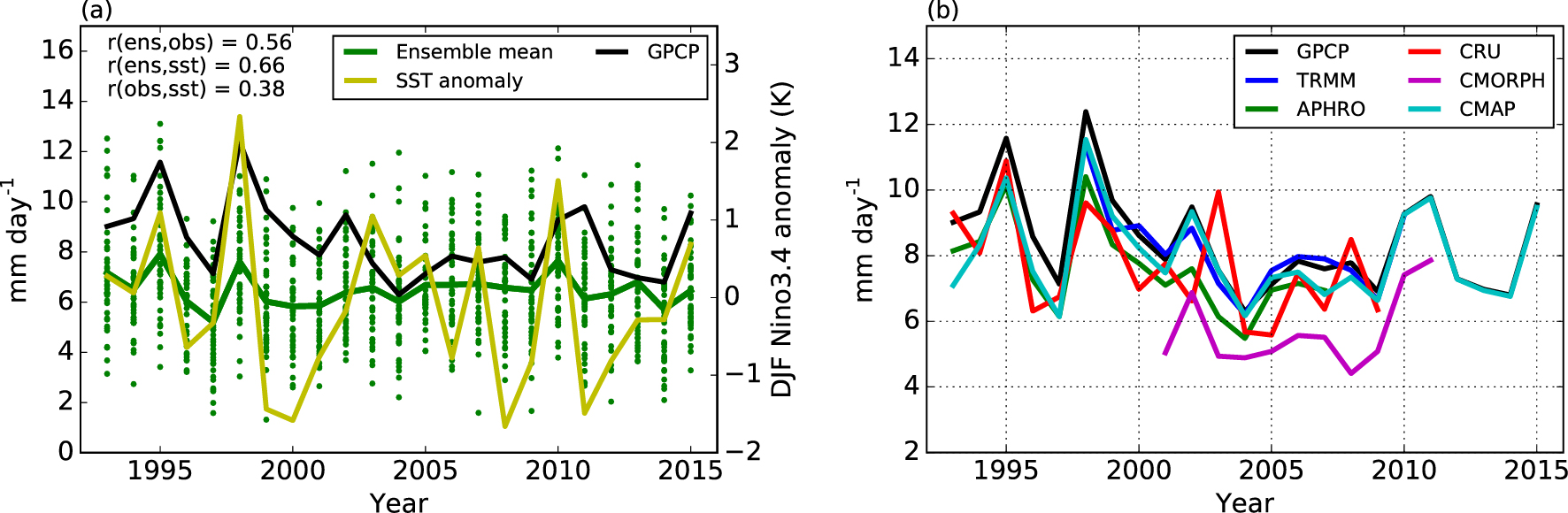 Figure3. (a) Year-to-year prediction of June mean rainfall (units: mm d?1) in the middle/lower Yangtze River region (25°–32.5°N, 110°–120°E) from GloSea5 ensemble predictions initialized on 1, 9, 17 and 25 March (green dots represent individual members of the 44-member ensemble) and their ensemble mean (green line), compared with June mean rainfall from GPCPv2.3 (black line). r(ens, obs) indicates the Pearson correlation coefficient between the ensemble mean predicted rainfall and the GPCPv2.3 rainfall. The yellow line indicates the observed SST anomalies (units: K) from HadISST1.1 during the preceding DJF averaged over the Ni?o3.4 region (5°S–5°N, 170°–120°W). r(ens, sst) and r(obs, sst) indicate the Pearson correlation coefficients between the observed Ni?o3.4 SST in DJF and the predicted June mean rainfall and that from GPCPv2.3 respectively. (b) June mean rainfall in the middle/lower Yangtze River region from six observational datasets.
| Hindcast start dates/No. of members | s.d. (GPCP; mm d?1) | ||||
| February/40 | March/44 | April/56 | |||
| June | r | 0.50 | 0.56 | 0.52 | 1.50 |
| s.d. (ens) | 0.56 | 0.63 | 0.66 | ||
| s.d. (mem) | 1.92 (1.50, 2.36) | 1.93 (1.44, 2.43) | 2.00 (1.53, 2.48) | ||
| July | r | 0.25 | 0.19 | 0.12 | 1.58 |
| s.d. (ens) | 0.32 | 0.33 | 0.31 | ||
| s.d. (mem) | 1.66 (1.27, 2.06) | 1.71 (1.30, 2.16) | 1.75 (1.32, 2.20) | ||
| August | r | 0.04 | 0.11 | ?0.03 | 1.02 |
| s.d. (ens) | 0.27 | 0.35 | 0.31 | ||
| s.d. (mem) | 1.51 (1.15, 1.88) | 1.54 (1.17, 1.91) | 1.68 (1.26, 2.13) | ||
Table1. Skill for predicting rainfall in the middle/lower Yangtze River region (25°–32.5°N, 110°–120°E) in June, July and August from GloSea5, using GPCPv2.3 observations as the reference, for different hindcast start dates. Start dates are 1, 9, 17 and 25 of the month. Pearson correlation coefficients (r) that are statistically insignificant (for a 23-year hindcast period) at the < 5% level for a one-tailed t-test are set in italics. Also shown is the interannual standard deviation (in mm d?1) of the hindcast ensemble means [denoted s.d. (ens)] and the average interannual standard deviation (in mm d?1) over 10?000 pseudo time series created by randomly selecting individual ensemble members for each year [denoted s.d. (mem)]. Values in parentheses indicate the (5th, 95th) percentile values from the 10?000 pseudo time series. The final column shows the interannual standard deviation of monthly mean rainfall from GPCPv2.3.
Similar analysis is carried out for the combined ensembles comprised of the four start dates in February and April. Table 1 shows that the correlation coefficients are all consistently > 0.5, indicating significant skill at the < 1% significance level (for a one-tailed t-test) for lead times of up to 4 months.
2
3.4. Robustness of skill
To assess the influence of ensemble size on the prediction skill of June mean rainfall, we randomly sample small ensembles of increasing numbers of members from each of the ensembles with start dates in February, March and April, and recalculate the correlation between the ensemble-mean time series and that from the observations for different ensemble sizes. Figure 4 shows that the prediction skill rises quickly with ensemble size, exceeding the 1% significance level in the ensembles from all start dates for a 30-member ensemble or larger, and is robust (correlation coefficients averaged over all ensemble-mean time series are statistically significant at the 5% level for a one-tailed t-test) for around 10 ensemble members or more. In contrast, Table 1 illustrates that there is no significant skill for this region in July and August for any of the start dates analyzed. Table 1 also shows the interannual standard deviation of the observed and modeled monthly rainfall in July and August for the ensemble means and from 10?000 pseudo time series created by randomly selecting individual ensemble members for each year. This shows that, while the interannual variability of the monthly mean rainfall is captured reasonably well by individual ensemble members, the interannual standard deviation of the ensemble mean rainfall is considerably smaller than observed in July and August. This, combined with the low skill in these months, suggests that other sources of rainfall (such as tropical cyclones), occurring after the break that follows the end of the mei-yu, may dominate the July and August mean rainfall and that, while they may be represented by the model in individual ensemble members, they are less predictable on seasonal time scales.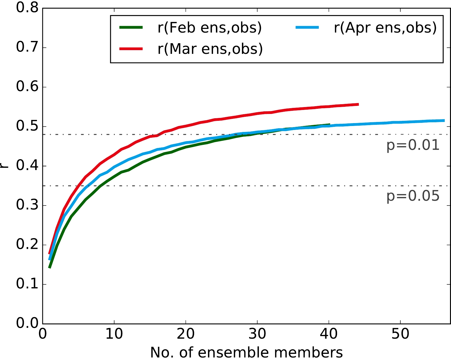 Figure4. Effect of ensemble size on the skill of June mean rainfall predictions over the middle/lower Yangtze River region. Curves indicate the correlation between ensemble means from start dates in February, March and April and GPCPv2.3 observations, denoted r(month ens, obs). For each choice of ensemble size, 10?000 ensemble-mean pseudo time series are generated by randomly selecting the chosen number of ensemble member June mean rainfall predictions (independently and without replacement) from all of the individual June mean rainfall values diagnosed in each year in the combined ensemble and averaging over the chosen number of ensemble members. Thin horizontal dot-dashed lines indicate the values of r that are significant at the 1% and 5% levels for a one-tailed t-test.
In order to assess whether the skill for predicting June mean rainfall in the middle/lower Yangtze River region is useful, we provide a contingency table (Table 2) illustrating the “hit rate” and “false alarm” rate for above-normal and below-normal rainfall predictions respectively, along with an overall score, for the combined predictions made using February, March and April start date ensembles. This illustrates that the forecasts are useful (in the sense of being of the correct sign) in more than half of the above-normal and below-normal cases, with the forecasts being useful 58% of the time overall.
| Ensemble means from Feb, Mar and Apr start dates (23 years) | Observed | ||
| Above average (3 × 11 years) | Below average (3 × 12 years) | ||
| Predicted | Above normal | 17 | 13 |
| Below normal | 16 | 23 | |
| Hit rate | 52% (17/33) | 64% (23/36) | |
| 58% (40/69) | |||
| False alarm rate | 36% (13/36) | 48% (16/33) | |
| 42% (29/69) | |||
Table2. Contingency table for hindcast predictions of June mean rainfall in the middle/lower Yangtze River region (25°–32.5°N) during 1993–2015. Event counts are based on the GPCPv2.3 observations and ensemble mean hindcasts for June using start dates in February, March and April, as shown in Table 1. The hit rate (false alarm rate) is the ratio of the number of hits for above-average or below-average rainfall to the number of times each of those conditions were observed (not observed). The overall hit rate (false alarm rate) is the ratio of the total number of successful (unsuccessful) hindcasts to the total number of samples (23 years × 3 ensemble means).
The presence of significant skill for prediction of June mean rainfall despite the climatological dry bias in this region is consistent with the conclusions of Scaife et al. (2019) for tropical seasonal mean rainfall. The skill for predicting June mean rainfall in the middle/lower Yangtze River region is also consistent with the findings of Li et al. (2016) for JJA rainfall over the large Yangtze River basin, suggesting that the skill for the season as a whole may be largely influenced by the contribution from the mei-yu rainfall in June. This perhaps reflects the particular characteristics of the mei-yu rainband—a distinct and unique feature of the EASM occurring as part of the seasonal progression of the subtropical high (Chen et al., 2004)—and its occurrence as a “stationary phase” in the seasonal evolution of the EASM (Ding and Chan, 2005) that is present in the middle and lower Yangtze River valley largely during June alone. The rainfall associated with the mei-yu is the main contributor to the June mean rainfall, and although the mei-yu rainy season extends into the first week of July, this does not appear to influence the skill for July. This suggests that other sources of rainfall (such as tropical cyclones), occurring after the break that follows the end of the mei-yu, dominate the July mean rainfall and are less predictable on seasonal time scales.
We investigate possible sources of skill in the next section.
The EASMI is strongly related to the strength of the WNPSH. Su et al. (2014) showed that the drivers of interannual variations in rainfall in southern China in the early summer are related to the position and strength of the WNPSH. Figure 5a shows the June mean 850-hPa winds from the ERA-Interim reanalyses regressed upon the GPCPv2.3 June mean rainfall anomalies in the middle/lower Yangtze River region (as used in section 3) between 1993 and 2015. Similar to the findings of Su et al. (2014, their Fig. 9), the circulation anomalies associated with increased June mean rainfall in the middle/lower Yangtze River region are characterized by an anticyclonic circulation anomaly over the SCS and the Philippine Sea and anomalous southwesterly winds across southern China and to the south of Korea and Japan. Figure 5a shows the two boxes used in the EASMI definition; it is clear that the main characteristics of the 850-hPa circulation anomalies associated with June mean rainfall variations in the middle/lower Yangtze River region will be captured by this index. Figure 5b shows a similar regression for the hindcast ensemble with start dates in March. The anomaly pattern agrees well with that from the observations/reanalyses, although the anomalies in the hindcast are rather stronger over the SCS and to the east of the Philippines and rather more westerly to the south of Japan.
 Figure5. (a, b) Regression of June mean 850-hPa winds onto June mean rainfall in the middle/lower Yangtze River region [shown by the red box in (c, d)] from (a) ERA-Interim and GPCPv2.3, and (b) GloSea5 ensemble member predictions initialized on 1, 9, 17 and 25 March. (c, d) Regression of June mean 850-hPa winds and rainfall from (c) ERA-Interim and GPCPv2.3, and (d) GloSea5 ensemble member predictions initialized on 1, 9, 17 and 25 March, onto observed preceding DJF Ni?o3.4 SST anomalies from HadISST1.1. In both cases, the regressions for GloSea5 are calculated for, and then averaged over, 10?000 single-member pseudo time series generated by randomly selecting an ensemble member (independently and without replacement) from all of the available ensemble members for each year in the combined ensemble with March start dates. The black boxes in (a, b) indicate the two regions used in the EASMI calculation. The values in each panel are scaled by the interannual standard deviation of the independent variable.
Wang et al. (2013) demonstrated that, on seasonal time scales, WNPSH variations are highly predictable by both physically based empirical models and dynamical models. Camp et al. (2019) demonstrated skill in GloSea5 for predicting the intensity of the WNPSH using the index proposed by Wang et al. (2013). Several other studies have also demonstrated skill for predicting the seasonal mean EASMI in various dynamical models, including GloSea5 (e.g., Li et al., 2012, 2018b; Liu et al., 2015, 2018). However, as noted by Wang et al. (2008), an advantage of the EASMI is that it can be monitored on a variety of time scales and is known to be an excellent indicator of variations in the SCS summer monsoon onset (Wang et al., 2004). Martin et al. (2019) recently demonstrated significant predictive skill for the SCS summer monsoon onset in GloSea5. We next investigate the predictive skill for the monthly mean EASMI in GloSea5.
2
4.1. Prediction skill for monthly mean EASMI
Figure 6 shows the prediction skill for the EASMI in June (using start dates in March) compared with the EASMI from ERA-Interim, while Table 3 shows the prediction skill for JJA for start dates in February, March and April. The EASMI from GloSea5 exhibits a noticeable negative bias compared with the values from ERA-Interim. This is related to the eastward extension and acceleration of the westerly outflow from the South Asian summer monsoon across the SCS and into the western Pacific in the model. Despite this systematic bias, the interannual variability of the predicted EASMI is realistic [the average interannual standard deviation of EASMI from 10?000 pseudo time series created by randomly selecting individual ensemble members for each year is 3.05 m s?1 (with a 5th to 95th percentile range of 2.37?3.75 m s?1), compared with 2.71 m s?1 for ERA-Interim], while the interannual variations in the ensemble mean predicted EASMI are somewhat smaller (interannual standard deviation of the ensemble mean predicted EASMI is 1.60 m s?1). For EASMI in June and August the prediction skill r(ens,ERAI) > 0.5 (p < 0.01), and in July r > 0.7 (p < 0.0001) (Table 3). Figure6. Prediction of June mean EASMI [difference in westerly winds at 850 hPa averaged over (22.5°–32.5°N, 110°–140°E) minus (5°–15°N, 90°–130°E)] from the GloSea5 ensemble initialized on 1, 9, 17 and 25 March (green dots represent individual members of the 44-member ensemble) and their ensemble mean (green line), compared with June mean EASMI from ERA-Interim (black line) and June mean rainfall over the middle/lower Yangtze River region (25°–32.5°N, 110°–120°E) from GPCPv2.3 (yellow line). r(pEASMI, ERAI), r(pEASMI, GPCP) indicate the Pearson correlation coefficients between the predicted EASMI and the ERA-Interim EASMI, and between the predicted EASMI and the GPCPv2.3 rainfall respectively.
| February | March | April | |
| June | 0.54 | 0.51 | 0.50 |
| July | 0.70 | 0.76 | 0.80 |
| August | 0.51 | 0.51 | 0.60 |
Table3. Skill for predicting the EASMI: Pearson correlation coefficients between the predicted EASMI in June, July and August from GloSea5 and that from ERA-Interim for hindcast start dates in February, March and April (1, 9, 17 and 25 of the month).
As suggested by Wang et al. (2008), in observations there is a strong relationship between the EASMI and the mei-yu rainfall on seasonal time scales. For 23 years of June mean rainfall from GPCPv2.3 in the middle/lower Yangtze River region used in the present study, the correlation with the EASMI from ERA-Interim is 0.48 (p = 0.01). This suggests that the skillfully predicted June mean EASMI from GloSea5 could be used as a proxy predictor for the June mean rainfall. Figure 6 and Table 4 show the skill for predicting the GPCPv2.3 June mean rainfall in the middle/lower Yangtze River region (25°–32.5°N, 110°–120°E) using the monthly predicted EASMI from GloSea5 as a proxy. The skill for predicting June mean rainfall using the EASMI from GloSea5 [r(pEASMI,GPCP)] is very similar to that for predicting the rainfall directly (see Table 1). There is also a similar lack of skill for predicting July and August mean rainfall in this region using the EASMI as a proxy (Table 4), despite the high skill shown in Table 3 for predicting the EASMI itself in these months. This highlights once again the lack of relationship between the EASMI and rainfall in this region in July and August, and provides additional confidence in the prediction skill for June rainfall using either proxy indices or explicit rainfall forecasts.
| February | March | April | |
| June | 0.50 | 0.52 | 0.58 |
| July | ?0.04 | 0.14 | 0.26 |
| August | 0.19 | ?0.24 | ?0.19 |
Table4. Skill for predicting June mean rainfall in the middle/lower Yangtze River region using the EASMI as a proxy: Pearson correlation coefficients between the predicted EASMI in June, July and August from GloSea5 and GPCP rainfall in the middle/lower Yangtze River region for hindcast start dates in February, March and April (1, 9, 17 and 25 of the month). Correlation coefficients statistically insignificant (for a 23-year hindcast period) at the < 5% level for a one-tailed test are set in italics.
2
4.2. Relationship with SSTs
Wang et al. (2008) stated that “the fundamental causes for interannual variation of EASM on seasonal timescales are the impacts of ENSO and the monsoon-warm pool interaction”. However, Chen et al. (2013) noted several studies indicating that the influence of ENSO on the EASM depends on the phase of ENSO, i.e., whether it is developing or decaying during the summer. The influence of ENSO has been shown to be greatest in the summer following a strong El Ni?o event (Wang et al., 2000, 2001; Wu et al., 2010; Xie et al., 2016; Hardiman et al., 2018). Hardiman et al. (2018) investigated this asymmetric relationship in terms of the seasonal mean Yangtze River basin rainfall. They showed that an anomalously strong anticyclone forms in the Northwest Pacific in summer (JJA) in response to an El Ni?o event in winter. This drives moisture-bearing winds northwards from the SCS, through Southeast China to the Yangtze River basin, leading to anomalously high precipitation there. In contrast, Hardiman et al. (2018) showed that there was no significant signal in the large-scale circulation, or the precipitation in the Yangtze River basin, following a winter La Ni?a event.Several studies (including Kim et al., 2008; Ye and Lu, 2011; Su et al., 2014; Li et al., 2018a) have further demonstrated that the teleconnection with ENSO SSTs varies subseasonally. Using a combination of observations and modeling, each of these studies demonstrated that the relationship with ENSO SSTs is strongest in early summer. Su et al. (2014) showed that rainfall anomalies associated with ENSO vary spatially and temporally according to the seasonal variation in the basic flow associated with the northward progression of the EASM. Their results suggested that the ENSO-related positive subtropical rainfall anomalies shift northwards with the upper-tropospheric westerly jet and the WNPSH between early and late summer, even under an almost identical tropical forcing. Further, the recent study by Li et al. (2018b) suggested that El Ni?o SST anomalies in the tropical Pacific during the previous winter, combined with SST anomalies in the Indian Ocean and the North Atlantic in spring that are often, but not exclusively, associated with a decaying El Ni?o, all contribute to atmospheric circulation anomalies over Eurasia and the western Pacific that influence the EASM rainfall in early summer.
Figure 5c shows the June mean 850-hPa winds from ERA-Interim and rainfall from GPCPv2.3 regressed onto the observed Ni?o3.4 SST anomalies for the period 1993–2015. Consistent with previous studies (e.g., Wang et al., 2009; Mao et al., 2011; Ye and Lu, 2011) positive December–January–February (DJF) Ni?o3.4 SST anomalies from the previous winter are associated with positive rainfall anomalies over southern China and negative anomalies over the SCS and to the east of the Philippines. These are themselves associated with an anomalous anticyclone over the SCS and the Philippines; this Philippine Sea anomalous anticyclone was described by Wang et al. (2000) and others as “the critical system that conveys delayed El Ni?o impact to the EASM” in the summer following an El Ni?o, and particularly in the early summer (Wang et al, 2009; Mao et al, 2011). Figure 5d shows similar analysis from the hindcast ensemble initialized using start dates in March. The pattern of rainfall and circulation anomalies is captured fairly well, although it is generally shifted slightly to the south. Figure 5c also shows a small region of negative rainfall anomalies over the Yellow Sea and the Sea of Japan associated with an anomalous cyclonic pattern. This was also seen in the analysis of Mao et al. (2011) and Wang et al. (2009), but is not captured by the hindcast.
The correlation between June mean rainfall from GPCPv2.3 and the preceding observed DJF Ni?o3.4 SSTs for the period 1993–2015 is r(obs, sst) = 0.38 (p < 0.05). This indicates that there are other factors than the preceding winter’s Ni?o3.4 SSTs that are influencing the June mean rainfall anomalies in the observations, such as snow anomalies over Eurasia (Wu et al., 2009) and the Tibetan Plateau (Ren et al., 2016), and intraseasonal and synoptic variability (Ding and Chan, 2005). For the GloSea5 hindcast ensemble initialized with start dates in March, the average correlation between the preceding DJF Ni?o3.4 SSTs and 10?000 pseudo time series of June mean rainfall generated by randomly choosing an individual ensemble member hindcast for each year from the ensemble initialized with start dates in March is r(members, sst) = 0.21, with a 5th to 95th percentile range of ?0.13 to 0.52 (see Table 5 for similar analysis with the February and April start dates), indicating that the influence of the DJF Ni?o3.4 SSTs on the June mean rainfall in individual ensemble members is slightly lower than r(obs, sst). This may indicate that the model is capturing some, but not all, of the other factors influencing the June mean rainfall, or that the internal variability in the model is larger than in reality (consistent with the larger interannual variability of June mean rainfall across the ensemble described in section 3.3).
| February | March | April | |
| r(members, sst) | 0.15 (?0.19, 0.48) | 0.21 (?0.13, 0.52) | 0.21 (?0.12, 0.52) |
| r(ens, sst) | 0.53 | 0.66 | 0.66 |
Table5. Modeled relationship between predicted June rainfall in the middle/lower Yangtze River region and observed winter ENSO SSTs: Average of Pearson correlation coefficients [r(members, sst)] between the observed preceding DJF Ni?o3.4 SSTs and 10?000 pseudo time series of June rainfall generated by randomly choosing an individual ensemble member hindcast for each year from the ensembles initialized with start dates in February, March and April (1, 9, 17 and 25 of the month). Numbers in parentheses indicate the (5th, 95th) percentile values. The correlation coefficient between the ensemble mean predicted June rainfall and the observed DJF Ni?o3.4 SSTs is indicated as r(ens, sst).
There are strong correlations between the ensemble mean predicted rainfall and the observed SST anomalies in the Ni?o3.4 region during the preceding DJF [r(ens, sst); see Table 5]. There is particularly good agreement between the ensemble mean predicted rainfall and both the observed rainfall anomalies and the winter Ni?o3.4 SST anomalies during summers following large El Ni?o events (e.g., 1995, 1998, 2010) (Fig. 3). This suggests that the winter Ni?o3.4 SST anomalies are driving the forced June mean rainfall signal in the model, consistent with the previous studies described above.
Both Hardiman et al. (2018) and Liu et al. (2018) showed that the seasonal mean EASMI, and its relationship with the preceding winter’s ENSO SSTs, are predicted skillfully by GloSea5. Good agreement is also found between the ensemble mean predicted June EASMI and that from ERA-Interim (Fig. 6) in the summers following strong El Ni?o events (1998 and 2010), with a small ensemble spread indicating that the EASMI in individual members responded strongly to this SST forcing. The average correlation between the preceding DJF Ni?o3.4 SSTs and 10?000 pseudo time series of June mean EASMI generated by randomly choosing an individual ensemble member hindcast for each year from the ensemble initialized with start dates in March is r(EASMImembers, sst) = 0.38, with a 5th to 95th percentile range of 0.09–0.64 (see Table 6 for similar analysis with the February and April start dates), which is statistically similar to the correlation between the June EASMI from ERA-Interim and the DJF Ni?o3.4 SSTs [r(ERAI, sst) = 0.30].
| February | March | April | |
| r(EASMImembers, sst) | 0.41 (0.11, 0.65) | 0.38 (0.09, 0.64) | 0.41 (0.12, 0.65) |
| r(pEASMI, sst) | 0.78 | 0.74 | 0.73 |
Table6. Modeled relationship between predicted June EASMI and observed winter ENSO SSTs: Average of Pearson correlation coefficients [r(EASMImembers, sst)] between the observed preceding DJF Ni?o3.4 SSTs and 10?000 pseudo time series of June EASMI generated by randomly choosing an individual ensemble member hindcast for each year from the ensembles initialized with start dates in February, March and April (1, 9, 17 and 25 of the month). Numbers in parentheses indicate the (5th, 95th) percentile values. The correlation coefficient between the ensemble mean predicted June EASMI and the observed DJF Ni?o3.4 SSTs is indicated as r(pEASMI, sst).
Once again, there are strong correlations between the ensemble mean predicted June EASMI and the observed preceding DJF Ni?o3.4 SSTs, r(pEASMI, sst) (see Table 6). This indicates that the model is able to represent the known influence of the preceding winter’s equatorial Pacific SSTs on the large-scale circulation of the WNPSH and the major influence that this has in determining the June mean rainfall in the middle and lower Yangtze River Basin region.
The potential for predictability of rainfall on subseasonal timescales has been discussed in several studies over the past decade (e.g., Kim et al., 2008; Wang et al., 2009; Ye and Lu, 2011; Yim et al., 2014). The existence of predictability on monthly time scales for the middle/lower Yangtze River basin region is related to the particular characteristics of the mei-yu rainband—namely, its occurrence as a “stationary phase” of the seasonal progression of the EASM (Ding and Chan, 2005) that is present in the middle and lower Yangtze River basin largely during June alone. Interannual variations in mei-yu rainfall have been linked in many previous studies to the circulation associated with the WNPSH, whose position and strength determine the southwesterly monsoon flow over southern China in early summer. The WNPSH has a known association with ENSO, with its influence depending on the phase and stage of development/decay (Huang and Wu, 1989; Wang et al., 2000; Wu et al., 2003; Feng et al., 2011; Chen et al., 2013; Su et al., 2014; Xie et al., 2016; Hardiman et al., 2018; Li et al., 2018a). As Wang et al. (2008) pointed out, while the EASM rainband migrates northwards during the summer, the interannual variability of the rainfall is a “persistent” mode with an anomaly pattern related to the variations in the large-scale EASM that persists through the whole summer.
Wang et al. (2008) demonstrated that variations in the low-level circulation around the WNPSH are adequately captured by the EASMI. Recent studies have demonstrated skill for predicting the seasonal mean EASMI in various dynamical models, including GloSea5 (e.g., Li et al., 2012, 2018b; Liu et al., 2015, 2018). We demonstrate here that significant skill is also present in GloSea5 for predicting the EASMI on monthly time scales, and that the latter can be used as a proxy to predict the regional rainfall. However, there appears to be little to be gained from using the EASMI as a proxy for regional rainfall on monthly time scales compared with predicting the rainfall directly.
While it is recognized that the mei-yu rainfall is influenced by synoptic events, intraseasonal variability and regional air–sea interactions with little or no predictability on the seasonal time scale, the ability to predict the June mean rainfall in the middle and lower Yangtze River basin region in GloSea5 at lead times of up to 4 months offers exciting possibilities for providing useful, early information to contingency planners on the availability of water during the summer season. We would encourage other forecasting centers to investigate the skill for predicting June mean rainfall in their operational forecasting systems.
Acknowledgements. This work and its contributors were supported by the UK–China Research and Innovation Partnership Fund through the Met Office Climate Science for Service Partnership (CSSP) China as part of the Newton Fund.
Open Access This article is distributed under the terms of the Creative Commons Attribution License which permits any use, distribution, and reproduction in any medium, provided the original author(s) and the source are credited.
