HTML
--> --> -->The X-band dual linear polarimetric doppler weather radar (hereafter referred to as X-POL) has received much attention in recent years and been applied as a useful supplement to operational radars. Because the polarization signatures of melting snowflakes are obviously different from those of raindrops and the wave scattering at the X-band is a non-Rayleigh scattering regime, X-POL is more sensitive to the characteristics of the BBML. Traditional methods often use the profile of polarimetric parameters to identify the BBML, such as VPR, VPDR (vertical profile differential reflectivity), and the VPC (vertical profile correlation coefficient). There are few algorithms for BBML recognition using X-POL in China. In this paper, the Bayesian method is developed and applied for X-POL to identify the BBML in Beijing.
Following this introduction, section 2 illustrates the specification, distribution and data credibility of X-POL. The data processing, images and statistical characteristics in the bright band of ZH, ZDR and CC observed by X-POL are described in section 3. The principles and steps of ML identification by the Bayesian method are presented in detail in section 4, which includes how to utilize the independent probability density distribution (IPDD) and joint probability density distribution (JPDD) of ZH, ZDR and CC to improve ML identification. Using the presented method, in section 5, a weather process that embodies the BBML is analyzed to verify the identification result. In section 6, the improvements in hydrometeor classification with the BBML detection are assessed. Finally, in section 7, a summary and some discussion of the Bayesian method for X-POL ML identification are provided.
 Figure1. The distribution of Beijing X-POLs, where the circles indicate the radar detection ranges of the X-POLs (60 km).
| Specification | Parameter (s) |
| Transmitter | Klystron |
| Frequency | 9.3–9.5 GHz |
| Wavelength | 3.2 cm |
| Peak power | ≥ 70 kW |
| Average power | 112 W |
| Max. duty ratio | 0.16% |
| Antenna diameter | 2.4 m |
| Beam width | 0.94° |
| Polarization mode | Linear horizontal and vertical; simultaneous transmission and reception |
| Detection range | 150–230 km |
| Gate width | 75 m |
| Max. pulse width | 0.5 μs |
| Detection parameters | ZH, Vr, Sw, ZDR, CC, ΦDP, and SNR |
Table1. The main performance parameters of X-POL.
The data are preprocessed by attenuation correction and de-noised by wavelet analysis (Hu et al., 2010; Hu and Liu, 2014), and the processing methods are briefly described in the following subsections.
2
2.1. Attenuation correction
The attenuation effect on radar ZH and ZDR at the X-band is substantial and cannot be ignored. The path-integral attenuations are compensated for by adding the attenuation to the measured ZH and ZDR as follows:where


where Zh =


2
2.2. Wavelet de-noising
The random fluctuation is reduced using wavelet de-noising with the following steps: (1) Deconstruction: each radial data is deconstructed into five levels with a db5 wavelet function. (2) De-noising: the detail coefficients in each level are suppressed with a ФDP penalty strategy. (3) Reconstruction: the data are reconstructed by means of an approximation and the processed detail coefficients with a soft function scheme. Once the data have been processed with the aforementioned attenuation correction and denoising, they are analyzed for BBML identification, as described in the following sections.2
2.3. Data reliability
According to the physical meaning of ZDR, the ZDR value in light rain should be approximately equal to zero. In order to verify the reliability of ZDR, some light rain data are selected in three precipitation processes. The criteria for light rain echoes are: signal to noise ratio (SNR) > 20 dB; slant range between 10 km and 20 km away from the radar; ZH < 15 dBZ; and CC > 0.98. After finding the gates that meet the light rain criteria, and averaging these gates of ZDR, SNR and CC, the maximum average value of ZDR is 0.12 dB and the minimum is 0.06 dB, as shown in Table 2. All the average values of ZDR are close to zero, which indicates there is almost no systematic deviation in the ZDR value.| Date | Gates | ZDR (dB) | SNR (dB) | CC |
| 12 August 2017 | 135 990 | 0.06 | 21.4 | 0.993 |
| 11 July 2018 | 124 738 | 0.12 | 20.5 | 0.996 |
| 15 October 2018 | 152 678 | 0.08 | 21.5 | 0.995 |
Table2. The ZDR biases estimated by the light rain method in three precipitation processes.
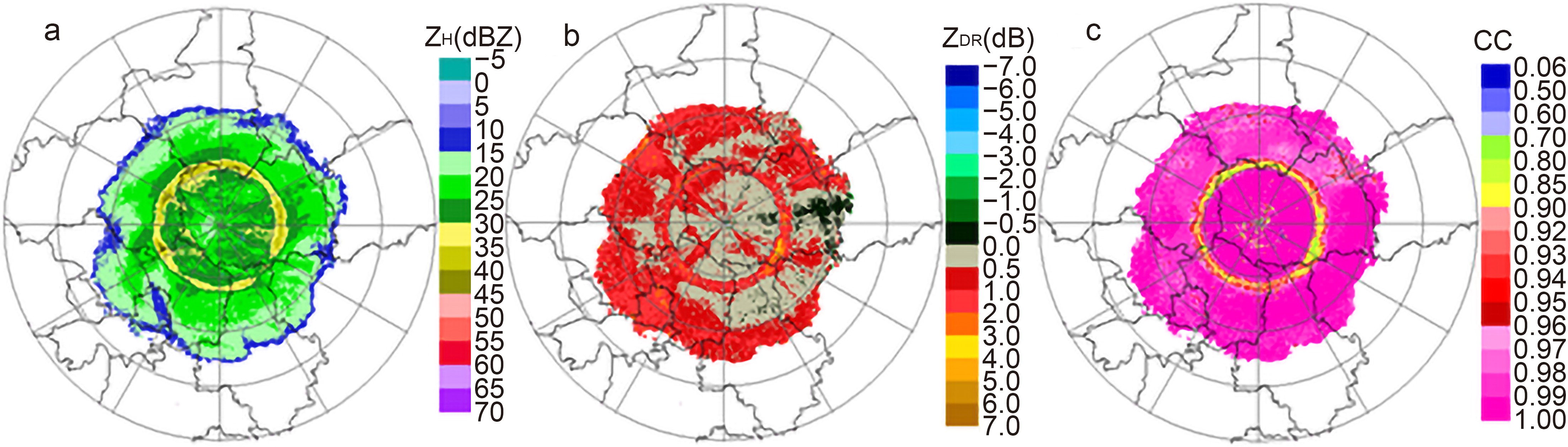 Figure2. The PPIs of (a) ZH, (b) ZDR, and (c) CC of X-POL in 9.9° at 0030 UTC 30 August 2018, in Shunyi, Beijing.
As a reminder, the partial criteria of Giangrande et al. (2008) for designation of ML boundaries is: the heights that encompass a majority of the ML points are determined. In the proposed algorithm, the ML top is determined as the height below which 80% of ML points reside. Similarly, the ML bottom is determined as the height below which 20% of the ML points reside. This algorithm is referred to as the MLDA (melting layer detection algorithm). The wavelength of the X-band radar is smaller than that of the S-band, so X-band radar is prone to non-Rayleigh scattering. When particles, such as wet snow with large diameters, are in the non-Rayleigh scattering regime, the electrical size of the particles is larger at the X-band than that at the S-band, which leads to a stronger non-Rayleigh scattering effect for the X-band radar observations. The larger differential scattering phase yields the reduced correlation of the dual polarization signals, leading to obvious differences in the values of ZH, ZDR and CC observed in the BBML from these at the S-band. The ZH values are distributed from 20 to 30 dBZ within the bright band region in azimuths from 120° to 150° (Fig. 2). There are obvious errors when determining the BBML points by using the MLDA algorithm based on the S-band WSR-88D ZH [ZH ∈ (30, 47) dBZ], which is not applicable to identifying BBML with X-POL measurements. In other words, most of the values are smaller than 0.90 in the PPI of the CC. This is also quite different from the values of the BBML points [CC ∈ (0.90, 0.97)] identified by the S-band WSR-88D. Therefore, it is necessary to redefine the distribution range of the BBML points using the bright band data observed with X-POL. According to the data from the slant ranges from 10 to 30 km in Fig. 2, the distributions of ZH, ZDR and CC are calculated and shown in Fig. 3. As seen from Fig. 3, most of the CC values are above 0.98 in the rain region from approximately 10 to 20 km. When the slant ranges are approximately from 20 to 22.5 km, which approaches the BBML, the CC values begin to decrease, and the minimum can reach 0.7. Therefore, the slant range of the BBML is roughly located from 20 to 25 km, where the CC values are mainly distributed from 0.70 to 0.96. The CC values increase gradually from 22.5 to 25 km and are mostly above 0.96 in the dry snow region, where the slant range is approximately 25 to 30 km.
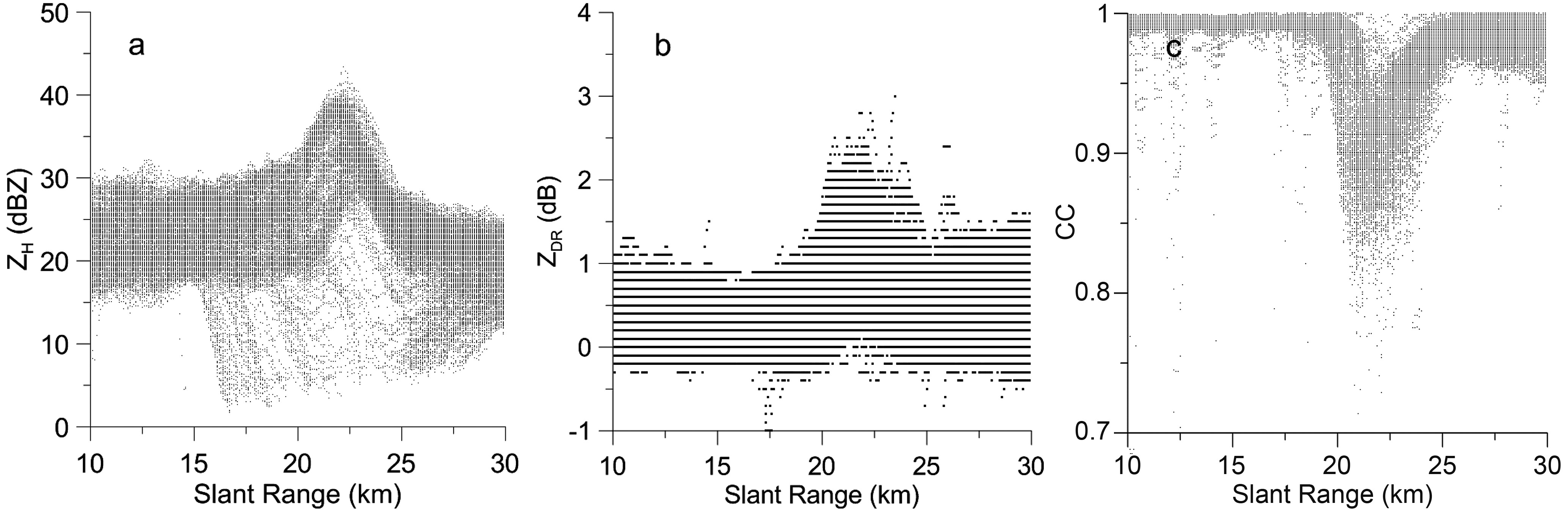 Figure3. Distributions of (a) ZH, (b) ZDR and (c) CC corresponding to Fig. 2.
ZH and ZDR are consistent with the characteristics of the BBML; both first increase and then decrease in the range of the BBML from 20 to 25 km, where the values of ZH are mainly distributed from 15 to 46 dBZ and those of the ZDR are from ?0.2 to 3.0 dB. However, the values of the ZDR are from 0.80 to 2.5 dB for WSR-88D. Therefore, the X-POL parameter thresholds are different from those of the WSR-88D polarimetric radar. Although the values of the polarimetric parameters in the BBML are mainly distributed within a certain scope, they are more reasonable after statistical processing because the boundary is not completely determined.
4.1. BBML identification principle based on the Bayesian method
The Bayesian method can be used to identify the ML if the distributions of the probability densities of the ZH, ZDR and CC in the ML region are known in advance. The steps of BBML identification are described as follows (Zhang, 2016): The radar echoes are divided into two categories, C = (BB, NB), in which the ML echo is represented by BB and the non-melting layer (NML) echo is represented by NB. The identification vector,


where Ci = (BB, NB), and p(


Based on the assumption that the classification is independent in a simple Bayesian identification, the conditional probability density can be decomposed into:
If it is assumed that the distribution of parameters in the observed discriminant vector


2
4.2. Obtaining the prior probability distribution
To obtain the probability density distributions (PDDs) of the ZH, ZDR, and CC in the BBML, the ML data observed by Shunyi X-POL shown in Table 3 are analyzed, and their prior PDDs are acquired according to the characteristic values of the X-POL in the ML. There are 634 volume scan data that include the BBML in eight days, observed by the VCP21 model, which scans one volume every three minutes. The ML region is manually selected from the 9.9° PPI, and the data influenced by lightning rods are excluded. A total of 6?705?261 sets of data are identified as ML points, and 85?368?196 sets of data are identified as NML points in the PPI. Based on these data, the IPDDs of the ZH, ZDR and CC are shown in Fig. 4, where BB represents the ML and NB represents the NML. Figure 4 shows that the IPDDs of the ZH, ZDR and CC for BB are greater than zero for approximately ZH ∈ (5, 46) dBZ, ZDR ∈ (?0.30, 3.5) dB, and CC ∈ (0.75, 0.96). It can be seen from the diagram that the PDDs of ZH and CC in the ML and NML are quite different, which is very beneficial for distinguishing the BB from the NB.| Date | Time (UTC) | Number of volume scan data |
| 22 May 2017 | 0112–0730 | 121 |
| 25 July 2017 | 2130–2357 | 50 |
| 26 July 2017 | 0000–0400 | 81 |
| 12 August 2017 | 0206–0548 | 75 |
| 29 August 2018 | 2221–2357 | 32 |
| 30 August 2018 | 0000–0348 | 77 |
| 11 September 2018 | 0951–1233 | 54 |
| 15 October 2018 | 0518–1227 | 144 |
Table3. Melting layer data observed by Shunyi X-POL.
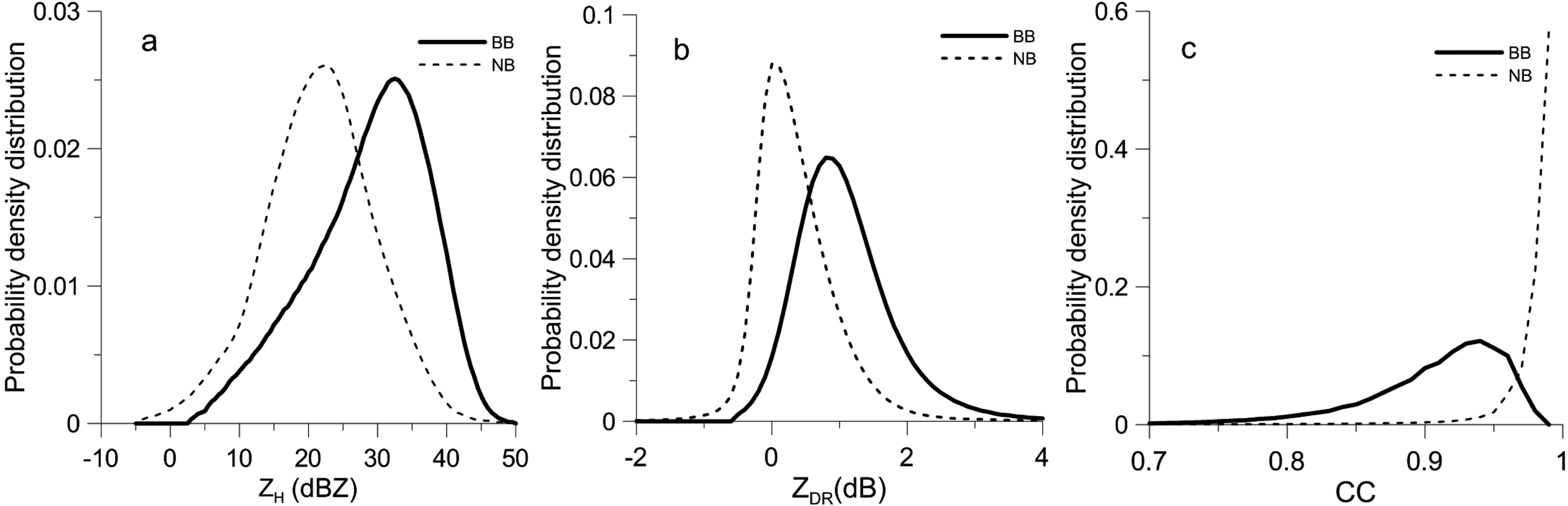 Figure4. The IPDDs of the ZH, ZDR and CC in the ML and NML.
The peak value of p(CC|BB) is located at CC = 0.93, which is obviously smaller than that of p(CC|NB) (approximately 0.98). The PDDs of the ZH and ZDR in the ML and NML partially overlap, but the ZH and ZDR values of the BBML are larger than those of the NML. Therefore, the PDD, combined with the ZH, ZDR and CC, can provide more information to distinguish the BB from the NB. Figure 5 shows the JPDDs of the ZH, ZDR and CC in the ML and NML, in which the differences in the JPDDs between the ML and NML are obvious and benefit distinguishing the BB from the NB.
 Figure5. The JPDD three-dimensional surface data map of (a1) ZH–ZDR, (a2) ZH–CC and (a3) ZDR–CC for BB. (b1–b3) As in (a1–a3) but for NB.
2
4.3. Singular point elimination
Because of the influence of ground clutter, some singularity points that are obviously non-melting points are often identified in the near surface by the above method, and these singularities need to be eliminated. The consistency check of the BBML identified by the Bayesian method is carried out to remove the singularity points that deviate from the center of the bright band thickness. The method of singularity elimination using the probability distribution is described as follows:The point value of (ZH, ZDR, CC) is substituted into Eq. (7) or Eq. (8), and the probabilities of BB and NB are obtained to determine whether the point is in the ML or NML by contrast with the PDDs in Figs. 4 and 5.
The upward float is 20% towards the height of the temporary bottom and the downward float is 20% towards the height of the temporary top according to all of the BBML points identified by step (1) in a certain PPI of the polarization radar, and the temporary thickness of each azimuth is obtained from the temporary bottom and top heights.
The median value, h, is calculated by sorting the results of the temporary thickness at each azimuth. Let σ = 2h; then, reidentify the BBML points in step (1) in the area determined by
where x is the height corresponding to each gate and f is the probability of a normal distribution.
Figure 6 shows the 9.9° PPI, which includes the BBML observed at 0500 UTC 11 July 2018 (unless specified, the following times and elevation angles are the same). Figure 6a shows the ZH and Figure. 6b shows the CC. The black color in Fig. 6c represents the result of the BBML recognition by the Bayesian method according to the IPDD, and the black color in Fig. 6e is according to the JPDD. It can be seen from Fig. 6 that the black rings identified as the BBML are very consistent with the decreasing CC region regardless of whether the ZH, ZDR and CC are based on the IPDD [Eq. (7)] or the JPDD [Eq. (8)] in the Bayesian method.
 Figure6. The PPIs of (a) ZH and (b) CC in 9.9° at 0500 UTC 11 July 2018 (unless specified, the following times and elevation angles are the same). The BBML points are shown in black according to the (c) IPDD and (e) JPDD. Panels (d, f) correspond to (c, e) after singular point elimination, respectively.
In the area far away from the BBML and near the radar station in Figs. 6c and e, there are points that are obviously mistakenly identified as the BBML due to ground clutter interference. There are more error recognition points in Fig. 6c than in Fig. 6e near the radar station, which indicates that the JPDD is better than the IPDD in suppressing the false recognition of ground clutter as ML points. The main reason is that the value of the CC is small, but the ZH and ZDR increase or decrease at the same time in the BBML; the CC value of ground clutter is also small, however the changes in the ZH and ZDR values are random. A consistency check is carried out on the BBML identified by the Bayesian method to remove the singularity points that deviate from the center of the bright band. Figures 6d and f show the results of eliminating singularity points corresponding to Figs. 6c and e, respectively. After eliminating the singularity points, there is a slight difference between Figs. 6d and f, but they are almost the same. The results of BBML identification are very consistent with the reduction band of the CC value in the PPI, which shows that both Bayesian methods, i.e., using IPDDs and JPDDs of (ZH, ZDR, CC), can effectively identify the BBML.
The bottom height of the zero-degrees layer is approximately 4600 m, and the top height is approximately 5000 m according to the sounding at 0600 UTC 11 July 2018. Figure 7 shows the ML height identified using the 9.9° PPI by the Bayesian method at 0415 UTC 11 July 2018, where Fig. 7a shows the IPDD result and Fig. 7b the JPDD result. In the figure, ML-Bot indicates the recognized ML bottom height, and ML-Top indicates the corresponding top height. Sou-Top and Sou-Bot are the heights of 0°C and 2.5°C obtained by sounding, respectively. There are slight differences between Figs. 7a and b, but the overall trend is consistent. The mean values of the bottom and top heights are 4590 m and 5009 m in Fig. 7a and 4575 m and 5027 m in Fig. 7b, respectively, which indicates that the performances of the two methods are similar.
 Figure7. Bottom and top heights of the BBML identified by the Bayesian method with the (a) IPDD and (b) JPDD.
For the MLDA of WSR-88D, the gate is considered as the BBML point when the values of ZH, ZDR and CC are ZH ∈ (30, 47) dBZ, ZDR ∈ (0.80, 2.5) dB, and CC ∈ (0.90, 0.97), respectively. As shown in Fig. 8c, the black color represents the recognized melting points by this MLDA, which are very limited. In the BBML of X-POL, most of the values of ZH are less than 30 dBZ, and the CC is less than 0.9, which do not satisfy the conditions of the ZH, ZDR and CC of the MLDA. Therefore, only a very small number of points are identified in the ML. This is mainly due to different scattering types between the X-band radar and S-band radar in the ML; X-band radar mainly results in Mie scattering, while S-band radar mainly results in Rayleigh scattering. Different scattering types lead to the ZH of the X-band being smaller than that of the S-band radar, but the ZDR of the X-band being larger than that of the S-band when the X-band and S-band radars detect wet snow in the same area. The scattering phase of the X-band radar is larger than that of the S-band radar, which makes the CC of the X-band radar smaller than that from the S-band radar. Therefore, the identification parameters for ML are different between the X-band and S-band radars.
 Figure8. The PPIs of (a) ZH, (b) ZDR and (c) CC in 9.9° at 0500 UTC 11 July 2018. The BBML points identified according to the MLDA of WSR-88D are shown in black in Fig. 8c.
According to the idea of the MLDA, with X-POL radar parameters of ZH ∈ (5, 46) dBZ, ZDR ∈ (?0.30, 3.5) dB, and CC ∈ (0.75, 0.96), the ML is reidentified. After finding the ML points, the ML top is determined as the height below which 80% of ML points reside, and the ML bottom is determined as the height below which 20% of the ML points reside. The black ring in Fig. 9a represents the BBML identified after the parameters are adjusted to X-POL. Figure 9b shows the results of the remaining points after limiting 20% and 80% of the BBML in Fig. 9a, and Fig. 9c shows the height of the BBML in each azimuth in Fig. 9b. It can be seen from Fig. 9c that some bottom heights of the BBML are lower than 1 km. Obviously, most of these points result from ground clutter, which has a great influence on BBML identification. In particular, the height of the ML top is obviously overestimated in azimuths from 203° to 209°.
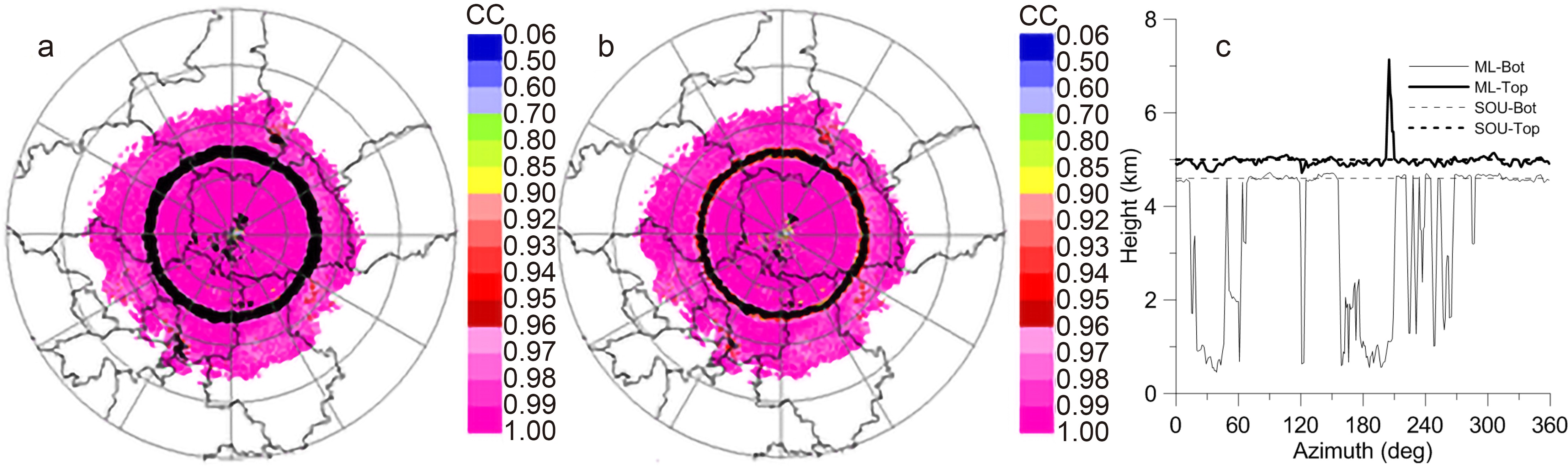 Figure9. BBML detection after the parameters are adjusted to X-POL (a), the results of the remaining parameters after limiting 20% and 80% of the BBML (b), and the height of the BBML in each azimuth (c).
The asymmetric or partial BBML in PPI images is selected to further verify the effect of the Bayesian method in identifying the ML. A case of asymmetric or partial BBML is displayed in Fig. 10, which shows the Fangshan radar of 9.9° PPI at 0130 UTC 11 July 2018. It can be seen from Fig. 10 that the BBML points identified by IPDD and JPDD correspond well to the ML area where the CC decreases. The result of Fig. 10 indicates that the Bayesian method can also effectively identify the asymmetric or partial BBML in the PPI.
 Figure10. The ZH (a), CC (b), and the BBML points (shown in black) according to the IPDD (c) and JPDD (d) of X-POL in 9.9° PPI at 0130 UTC 11 July 2018, in Fangshan, Beijing.
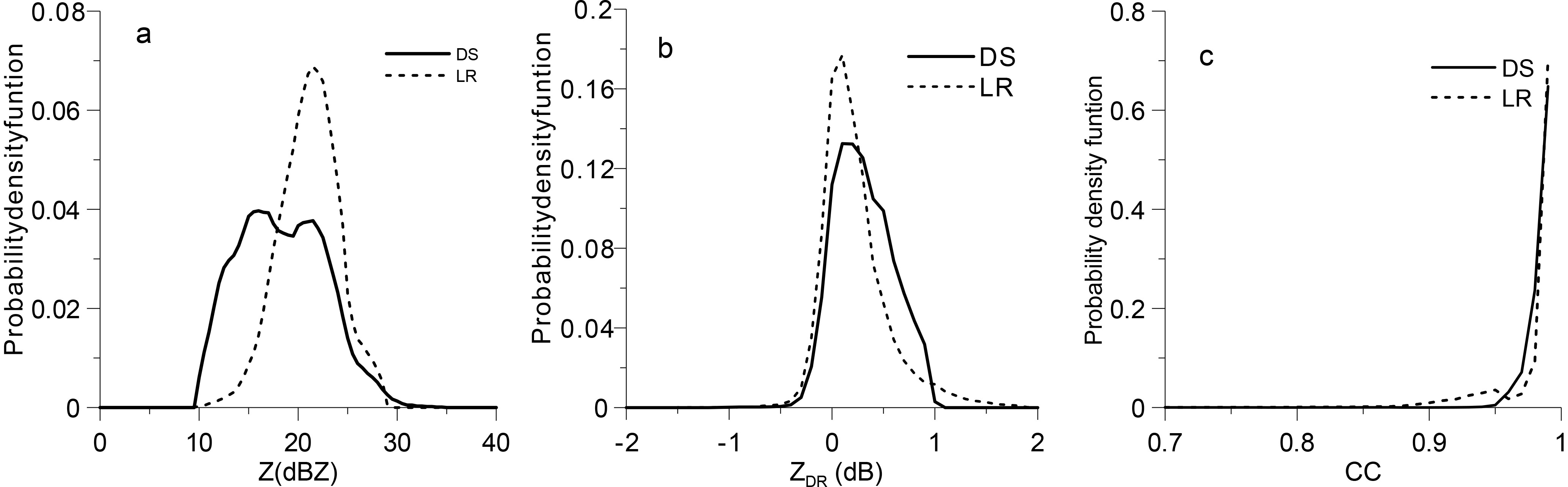 Figure11. The IPDDs of (a) ZH, (b) ZDR and (c) CC for light rain and dry snow.
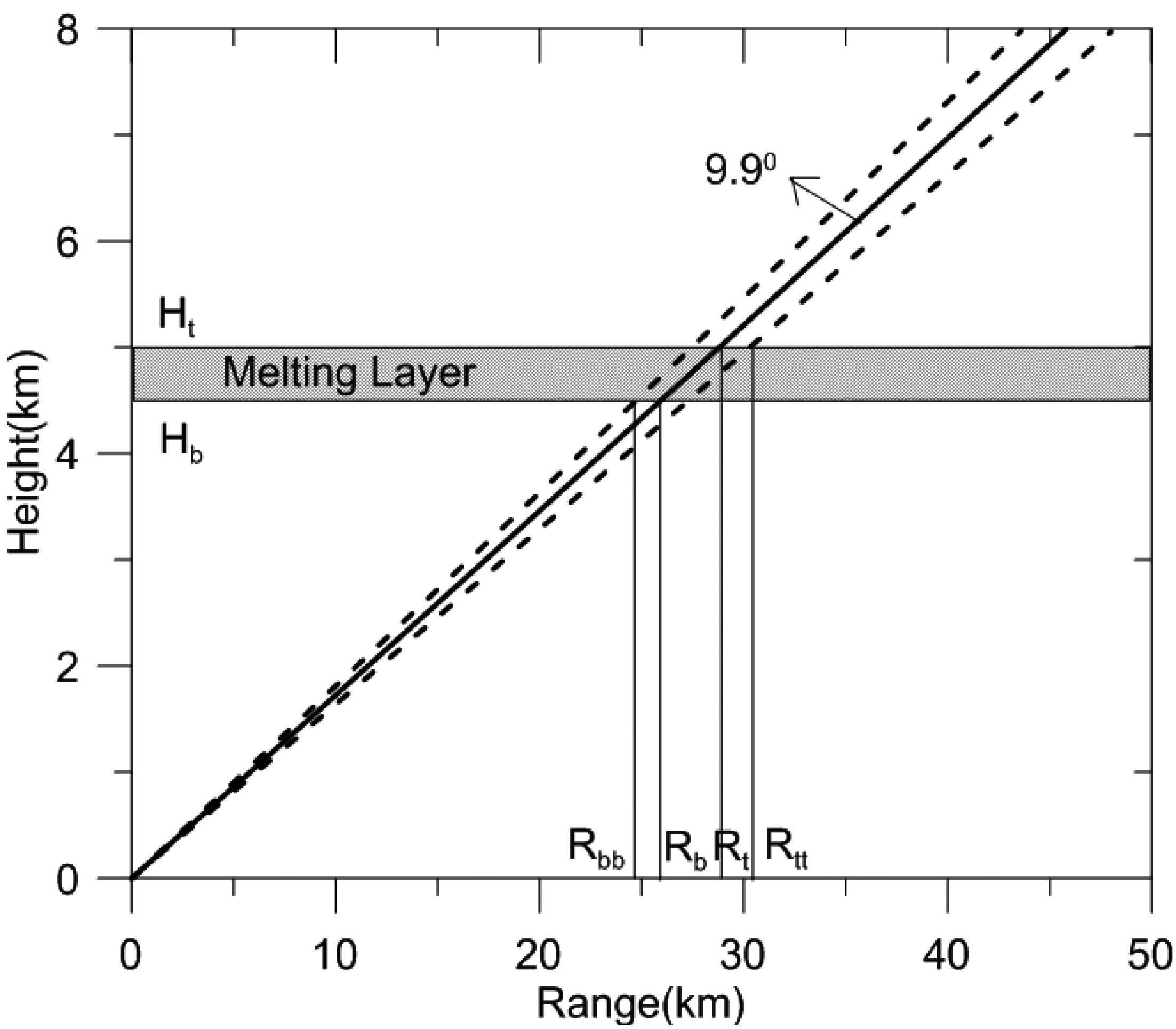 Figure12. Sketch of the intersection between beam broadening and the BBML. The heavy line represents the center of the radar beam at a 9.9° elevation angle, and the dashed line represents the ±0.5° beam width (3 dB beam width). Rbb, Rb, Rt and Rtt represent the slant range corresponding to the intersection points between the radar beam and the BBML; Hb and Ht represent the heights of the bottom and top of the BBML, respectively.
The hydrometeor particles are classified according to Table 4. Based on the distribution constraint relations of hydrometeor particles (Park et al., 2009), for a weather process in the BBML, the relationship between hydrometeor particles and the ML is as follows (R represents the slant range):
| Class number | 1 | 2 | 3 | 4 |
| Type | AP/GC | BS | DS | WS |
| Classification | Abnormal propagation or ground clutter | Biological scatter | Dry snow | Wet snow |
| Class number | 5 | 6 | 7 | 8 |
| Type | CR | GP | BD | LR |
| Classification | Ice crystals | Graupel | Big drops | Light rain |
| Class number | 9 | 10 | 11 | 12 |
| Type | MR | HR | RH | BH |
| Classification | Moderate rain | Heavy rain | Rain and hail | Big hail |
| Class number | 13 | 14 | ? | ? |
| Type | SH | CAE | ? | ? |
| Classification | Small hail | Clear air echo | ? | ? |
Table4. Hydrometeor particle-type classification.
0 < R < Rbb: the particles should not belong to dry snow, wet snow, ice crystals, or graupel;
Rbb < R < Rb: the particles should not belong to dry snow, ice crystals, light to medium rain, or heavy rain;
Rb < R < Rt: the particles should not belong to ice crystals, light to medium rain, or heavy rain;
Rt < R < Rtt: the particles should not belong to light to medium rain or heavy rain;
R > Rtt: the particles should not belong to ground clutter or abnormal propagation (e.g., hyper-refraction), biological scatter, wet snow, big drops, light to medium rain, or heavy rain.
Without the ML detection, when the slant range is R < Rbb, it is very difficult to distinguish light rain from dry snow by the fuzzy logic algorithm (Fig. 13a). Figure 13a shows the classification identification results, revealing obvious mistakes insofar as the dry snow appears below the BBML. After the BBML is identified by the Bayesian method, according to the constraint relation of the precipitation particle distribution above the BBML, there is light to moderate rain (mainly light rain) in the slant range of R < Rbb (Fig. 13b). In the BBML area, wet snow is identified as the main precipitation type, and the type distribution is reasonable, which improves the results of precipitation particle classification by the fuzzy logic method effectively.
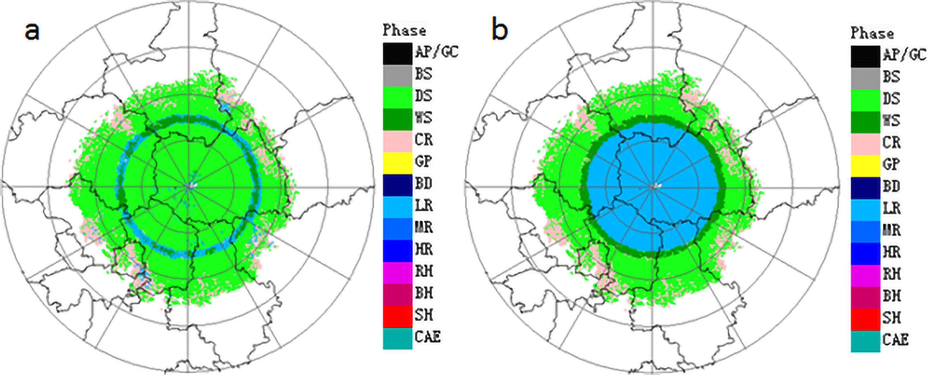 Figure13. Hydrometeor classification before (a) and after (b) BBML identification.
In order to further verify the influence of ML recognition on hydrometeors, the results of hydrometeor classification in Fig. 10 are shown in Fig. 14, which also show that the identification of BBML can improve the hydrometeor classification results of light rain and dry snow.
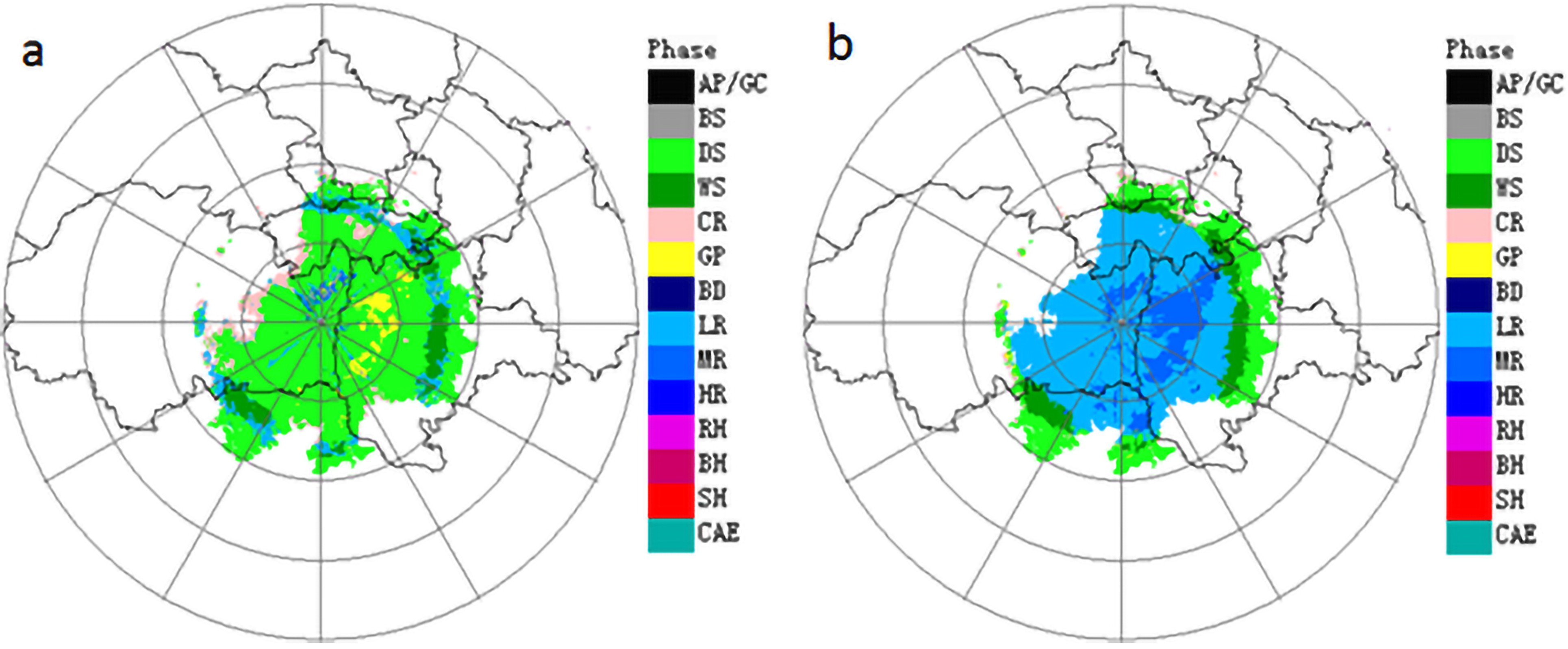 Figure14. Hydrometeor classification results in 9.9° PPI at 0130 UTC 11 July 2018 in Fangshan, Beijing, before (a) and after (b) BBML identification.
According to BBML identification by the data collected with the X-POL radar in Shunyi, Beijing, it is shown that the parameter ranges of the ML identification method are ZH ∈ (5, 46) dBZ, ZDR ∈ (?0.30, 3.5) dB, and CC ∈ (0.75, 0.96). However, the parameter ranges for the WSR-88D ML detection method are ZH ∈ (30, 47) dBZ, ZDR ∈ (0.80, 2.5) dB, and CC ∈ (0.90, 0.97). These parameter thresholds are significantly different from those of X-POL and cannot be simply applied to X-POL radars.
The case analysis shows that the Bayesian method can identify the BBML effectively, which plays an important role in hydrometeor classification. Because of the overlapping polarization parameters, it is difficult to distinguish dry snow from light rain using the fuzzy logic algorithm. However, the constraint relationship between dry snow, light rain, and the position of the ML provides much easier mutual identification.
Acknowledgements. This work was supported by a Beijing Municipal Science and Technology Project (Grant No. Z171100004417008), the National Key R&D Program of China (Grant No. 2018YFF0300102), and the National Natural Science Foundation of China (Grant Nos. 41375038 and 41575050).
