HTML
--> --> -->Wuhan is home to approximately 10 million inhabitants and has suffered from increasingly frequent haze pollution events in recent years. Based on one year of observations from March 2013 to February 2014 and data from the Chinese National Ambient Air Quality Standard, the number of days with a daily average PM2.5 concentration above 75 μg m?3 reached 193. This ranked Wuhan in fourth place among 31 provincial capital cities (Wang et al., 2014a). In fact, Wuhan’s annual average PM2.5 concentration of 92 μg m?3 is higher than that of Beijing (87 μg m?3), Shanghai (56 μg m?3), and Guangzhou (52 μg m?3) (Wang et al., 2014a). In particular, during the winter season, polluted days account for 90% of all days (Wang et al., 2014a). During the month of January 2013, the number of haze days was 25 in Beijing, while it was 30 in Wuhan during the same period (Zheng et al., 2015b). Persistently high concentrations of particulate matter (PM) are extremely harmful to human health. According to Chen et al. (2013), long-term exposure to ambient PM concentrations of approximately 184 μg m?3 can reduce life expectancy by more than three years in northern China. The number of premature adult mortalities due to excessive PM2.5 concentrations across China in 2013 was estimated to be greater than one million in total (Liu et al., 2016). Therefore, there is an urgent need to mitigate PM pollution in Wuhan and Central China.
To date, source apportionment studies for Wuhan have mainly been based on PM composition observations that can distinguish between sources from different sectors of activities or different types of fossil fuels (Cheng et al., 2012; Gong et al., 2015; Huang et al., 2015; Zhang et al., 2015; Lyu et al., 2016). Very few studies, however, have investigated the role of regional transport in the haze formation mechanism in Wuhan. For instance, Lu et al. (2017) employed a chemical transport model to quantify the contribution of regional transport to two pollution episodes in October 2014 and highlighted the complexity of the haze formation mechanism in Wuhan. However, further investigations on the source–reception relationship of Wuhan are needed—especially for haze episodes during the winter season.
Here, we examine an unprecedented long period of persistent pollution over Wuhan that took place in January 2014, and compare the relationship between the haze episodes and meteorological conditions in Wuhan with Beijing. Moreover, the influence of transboundary transport from the North China Plain (NCP), East China(EastC), and South China (SouthC)(definitions in section 2.2) was assessed to investigate the transport mechanism during this case in Wuhan. We used a high-resolution modeling system with an online source-tagged method validated by PM2.5 observations from 117 cities in Central and East China to perform the source apportionment of air pollution over Wuhan. It is the hope that regions with the highest contribution to Wuhan’s haze pollution are identified and are followed up by mitigation efforts. In addition, the clarification of pollution formation processes over the Wuhan area may help to establish a relationship of haze episodes between Wuhan and its surrounding city clusters and establish a holistic view of the joint evolution of pollutants across Central and East China. This is so that the integrated assessment and future development of polices can better cope with compound air pollution problems in China. Section 2 describes the methods and data used in this study. The observational features and formation mechanism of the haze episode are investigated in section 3. Section 4 provides conclusions and discussion.
2.1. Model description and simulation design
The Nested Air Quality Prediction Model System (NAQPMS), a 3D and multiscale air quality model from the Institute of Atmospheric Physics, Chinese Academy of Sciences, was employed to simulate the haze episode over Central and East China in January 2014 (Wang et al., 2006). The model can simulate physical processes (including horizontal and vertical advection and diffusion, dry and wet deposition) and chemical processes (including gaseous, aqueous and heterogeneous phase chemistry) of air pollutants with various modules (Li et al., 2007).The advection process and the dry deposition velocity were calculated referring to the algorithm of Walcek and Aleksic (1998) and a scheme of Wesely (1989), respectively. The RADM mechanism (Chang et al., 1987) was embedded into NAQPMS to address the wet deposition processes and aqueous phase chemistry. The gas chemistry module included 134 reactions with 71 species based on the “carbon-bond mechanism Z” (Zaveri and Peters, 1999). The six secondary organic aerosols were contained in NAQPMS with the methods and formation rates from Pandis et al. (1992) and Odum et al. (1997). Based on the results from previous studies, heterogeneous phase chemistry does play a significant part in the production of secondary inorganic aerosols during China’s winter season (Zheng et al., 2015a; Chen et al., 2016). The finding from Li et al. (2012) indicated that 28 heterogeneous chemical interactions on the surface of black carbon (BC), sulfate, dust, and sea salt particles were implemented in NAQPMS. In addition, version 3.6.1 of the Weather Research and Forecasting (WRF) model provided hourly meteorological data for simulating air pollutants in NAQPMS. The setup of the WRF model, including the model domains and their horizontal resolutions, was consistent with that in NAQPMS. Each domain contains 27 vertical levels stretched from the surface to 50 hPa. MODIS land-use data were used for the WRF modeling. The WRF physical parameterization schemes employed in this study included the Purdue Lin scheme (Lin et al., 1983; Rutledge and Hobbs, 1984) for the microphysical processes, the Grell-3 scheme for the cumulus parameterization, the Goddard shortwave radiation scheme (Chou and Suarez, 1994), the Rapid Radiative Transfer Model scheme for longwave radiation, the Noah land surface model, and the Yonsei University (YSU) planetary boundary layer scheme. The simulation period was from 0000 UTC 25 December 2013 to 0000 UTC 1 February 2014, and the first 24 hours were used as a spin-up period in a two-day simulation. NCEP-FNL data provided the initial and boundary conditions of the WRF model with a resolution of 1° × 1°. As shown in Fig. 1, three nested domains were set in WRF and NAQPMS, with horizontal resolutions of 27, 9 and 3 km, respectively. The mother domain covered Central and East China, the inner domain covered an area in Hubei and its nearby provinces, and domain 3 included Wuhan and surrounding cities in Hubei Province. The simulation of air pollutants was conducted from 25 December 2013 to 31 January 2014 with a spin-up period during the first seven days. The lateral boundary conditions for the first domain in NAQPMS was the monthly average data obtained by the global chemistry transport model MOZART-v2. They were kept constant during the simulation period and the boundary data in the nested domains were provided by their parent domains.
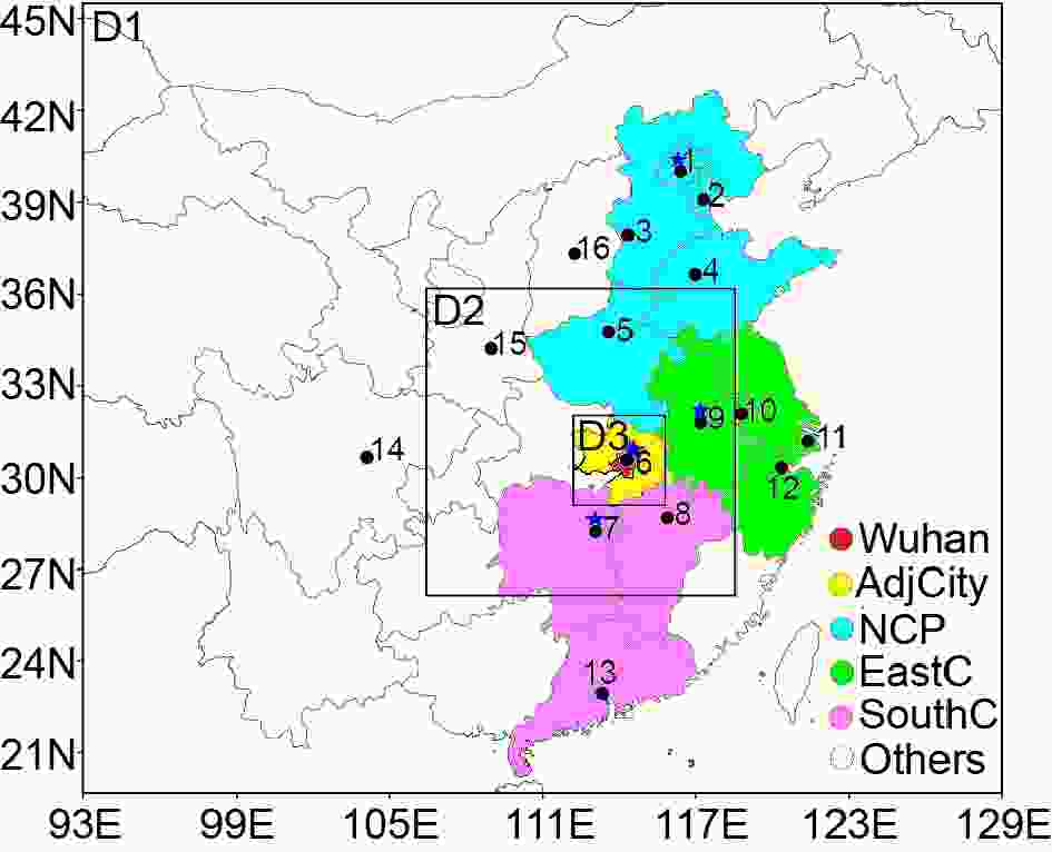 Figure1. Configuration of the three model domains and six tagged emission source regions. The North China Plain (NCP) includes Beijing, Tianjin, Hebei, Shandong and Henan provinces; East China (EastC) includes Shanghai, Jiangsu, Zhejiang and Anhui provinces; and South China (SouthC) includes Guangdong, Hunan and Jiangxi provinces. The eight cities surrounding Wuhan (AdjCity) include Ezhou, Xianning, Huanggang, Huangshi, Xiaogan, Xiantao, Tianmen, and Qianjiang. The locations of the four meteorological stations (blue stars) and sixteen PM2.5 level observation cities (black dots) are: 1-Beijing, 2-Tianjin, 3-Shijiazhuang, 4-Jinan, 5-Zhengzhou, 6-Wuhan, 7-Changsha, 8-Nanchang, 9-Hefei, 10-Nanjing, 11-Shanghai, 12-Hangzhou, 13-Guangzhou, 14-Chengdu, 15-Xi’an and 16-Taiyuan.
For analysis in section 3.2, the calculation of the atmospheric planetary boundary layer height (PBLH) in the YSU scheme of the WRF model is given. The PBLH is defined as the lowest height at which the overall Richardson number (


where


2
2.2. Source apportionment method
An online source-tagged algorithm (Li et al., 2008; Lu et al., 2017; Wu et al., 2017), similar to the Comprehensive Air Quality Model with Extensions/Particulate Source Apportionment Technology (Wagstrom et al., 2008), was employed to quantify the contributions of predefined source regions to the concentrations of air pollutants in Wuhan. The apportionments during the physical and aerosol chemistry calculations were separately calculated during the simulation. The method suffered a lower error compared to the traditional sensitivity method with the turning on/off of the emissions of the source-tagged regions due to the high nonlinearity of the chemical transport model. This method has been used in many previous studies to assess the influence of regional transport on the PM, ozone, and other gaseous species over different regions or cities (Wu et al., 2011; Li et al., 2013; Wang et al., 2014b; Li et al., 2016).In this method, the gaseous species and PM were assumed to be mixed well in each grid cell, and sharing the same loss coefficients during the outflow, chemical destruction, and dry and wet deposition. The secondary aerosols were simplified by connecting them directly to their corresponding precursors. Therefore, the fraction of each species (

where r and i are the tagged region and the index of the model cell, and


To quantify the regional contributions to the PM2.5 concentrations in Wuhan, we marked six emission source regions based on the administrative divisions shown in Fig. 1. The tagged source regions were: Wuhan and the eight nearby cities of Ezhou, Xianning, Huanggang, Huangshi, Xiaogan, Xiantao, Tianmen and Qianjiang; the NCP region, including Beijing–Tianjin–Hebei and the provinces of Shandong and Henan; EastC including the provinces of Shanghai, Jiangsu, Zhejiang and Anhui; SouthC including the provinces of Guangdong, Hunan and Jiangxi; and other areas, referred to simply as “others”.
2
2.3. Emission data
The anthropogenic emission data for NAQPMS was provided by version 2.1 of the Regional Emission Inventory in ASia (REAS) from Japan, covering East, Central, Southeast and South Asia with a spatial resolution of 0.25° × 0.25° (approximately 30 × 25 km) and a temporal resolution of one month (Ohara et al., 2007). The emission sources with the base years of 2000–08 included fuel combustion sources like heavy industry, power plants, transportation, and other activities of this kind, industrial emissions, agricultural activities such as fertilizer application and livestock, fugitive emissions, solvent use, and so on. The REAS emissions inventory is reported in detail in Kurokawa et al. (2013) and has been widely applied in numerical studies (Li et al., 2012; Zhong et al., 2014). For this case study of January 2014, a big obstacle was that the emissions inventory for the base year of 2014 was not available, while the emissions over China changed very rapidly due to the rapid urbanization, industrial development, and emission control measures. In order to reduce the uncertainty induced by the changes of regional emissions between 2008 and 2014, we employed the inverse method developed by Tang et al. (2013) and surface observations to update the regional emissions inventory for CO, SO2 and NOx. Figure S1 in Electronic Supplementary Material compares the CO simulations using the original and the inversed CO emissions inventory. The modeling errors of the precursors were greatly reduced, which could in turn reduce the uncertainties of the air pollutant transport modeling and improve the accuracy of the source apportionment results. Moreover, considering the significant impact of biomass burning across China (Ding et al., 2016), the daily fire emissions with 1-km resolution from the Fire Inventory from NCAR (FINNv1), including agricultural fires, wildfires, and prescribed burning (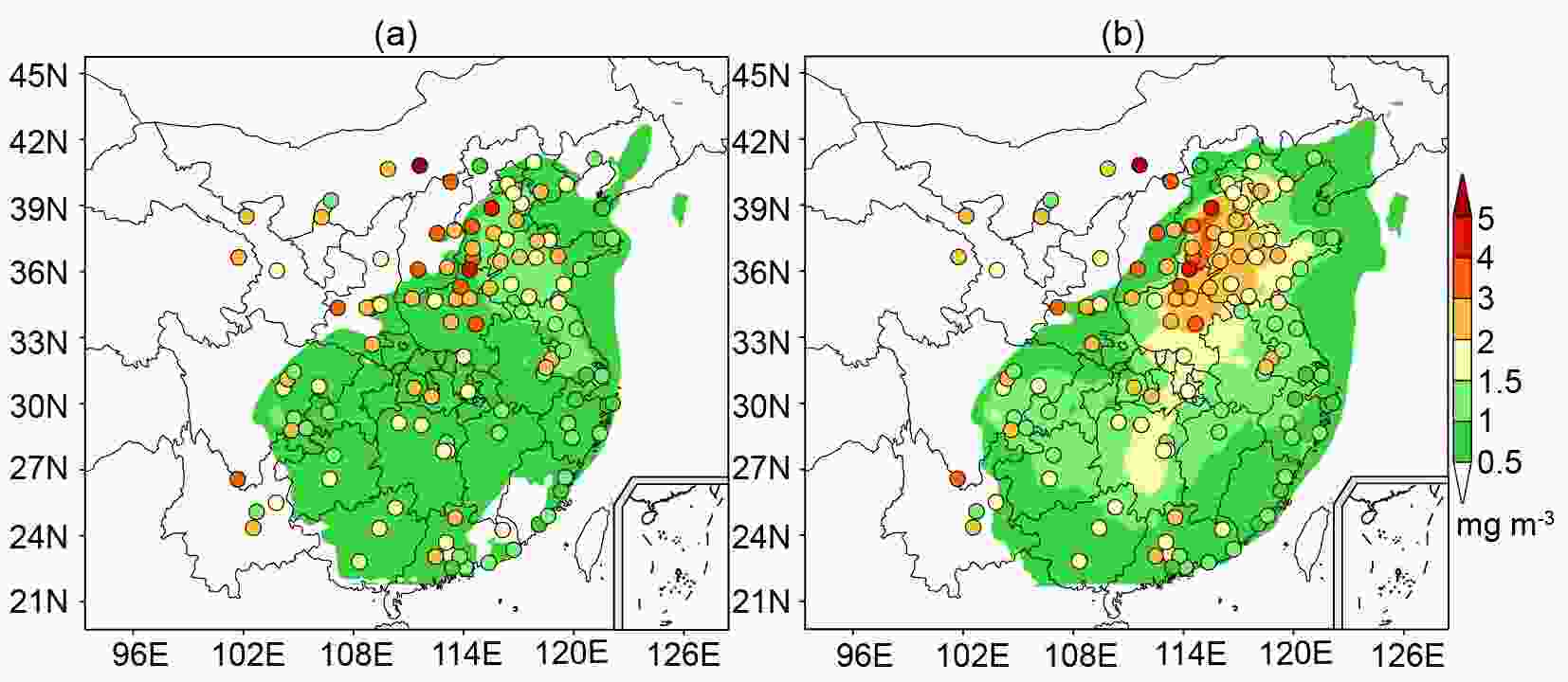 FigureS1. The distribution of simulated and observed average CO concentrations during haze pollution in January 2014 over Central and East China using (a) original and (b) inversed emissions.
2
2.4. Measurement data
Routine meteorological data in Wuhan and three other provincial cities (Beijing, Hefei, and Changsha) from the China Meteorological Administration were used to validate the WRF model and analyze the characteristics of the meteorological conditions in January 2014. The hourly observations, including 2-m temperature, 2-m relative humidity (RH), 10-m wind speed (WS) and wind direction (WD), were used. The hourly observed PM2.5 concentrations in Wuhan and 116 other cities were provided by the Wuhan Environmental Monitoring Center and the China National Environmental Monitoring Center, respectively. The locations of all observation stations are shown in Fig. 1. The data from these observation stations were used for validating NAQPMS and investigating the characteristics of the haze episode at both urban and regional scales.3.1. Model validation
To assess the performance of the WRF model for the meteorological simulations, the simulated surface temperature, RH, WD, and WS were compared with the observed data. Table 1 and Fig. S2 present the statistics of the model performance in Wuhan and other cities like Beijing, Hefei and Changsha. Overall, the WRF model was able to reproduce the main characteristics of the four meteorological variables in these four cities. The simulated temperatures at 2 m were close to the observations, with correlation coefficients (r) of 0.75–0.91 and average mean biases (MB) of approximately ?1.8 to 1.4°C. The variations of RH were also reproduced by the model with r values of approximately 0.72–0.84, except for more underestimation of RH in SouthC than that over the NCP. RH is a diagnostic quantity rather than an output of the model and is inferred based on the simulated temperature, surface pressure, and water vapor mixing ratio. As suggested by Yang and Duan (2016), one possible reason for the underestimation of RH in the WRF model is due to the overestimation of the surface temperature under insignificant change in water vapor pressure. WRF overestimated the surface temperature, with mean biases from 0.5°C to 1.4°C, in southern cities of China. The correlations between the simulated WSs and the observations, with r values ranging from 0.32 to 0.71, were relatively lower than those of temperature and RH, which might be related to the difficulty in simulating the weak atmospheric circulation at the urban scale. The WRF model was able to reproduce the evolution of the winds in these cities, especially for the period with prevailing strong winds.| Site | Factors | MO | MM | MB | r | MFB(%) | MFE (%) |
| Wuhan | T (°C) | 7.7 | 9.1 | 1.4 | 0.84 | 18.4 | 26.7 |
| RH (%) | 58.3 | 46.2 | ?12.1 | 0.77 | ?20.7 | 25.4 | |
| WS (m s?1) | 2.4 | 3.3 | 0.9 | 0.33 | 34.2 | 53.2 | |
| Changsha | T (°C) | 8.6 | 9.1 | 0.5 | 0.85 | 4.4 | 32.4 |
| RH (%) | 62.2 | 50.8 | ?11.4 | 0.84 | ?20.7 | 25.2 | |
| WS (m s?1) | 2.4 | 3.0 | 0.6 | 0.63 | 26.0 | 45.3 | |
| Hefei | T (°C) | 5.5 | 6.1 | 0.6 | 0.91 | ?15.6 | 17.4 |
| RH (%) | 68.3 | 56.3 | ?12 | 0.80 | ?18.2 | 24.7 | |
| WS (m s?1) | 1.9 | 3.2 | 1.3 | 0.71 | 58.3 | 62.4 | |
| Beijing | T (°C) | ?0.3 | ?2.1 | ?1.8 | 0.75 | 63.3 | ?55.8 |
| RH (%) | 44.3 | 40.8 | ?3.5 | 0.72 | ?0.8 | 31.6 | |
| WS (m s?1) | 2.0 | 2.9 | 0.8 | 0.32 | 36.3 | 59.6 |
Table1. Statistical parameters of the three simulated and observed meteorological parameters [temperature (T), relative humidity (RH), and wind speed (WS)] in Wuhan, Changsha, Hefei and Beijing in January 2014. The definitions of the abbreviations MO, MM, MB, r, MFB and MFE are given (Table S1 in Electronic Supplementary Material).
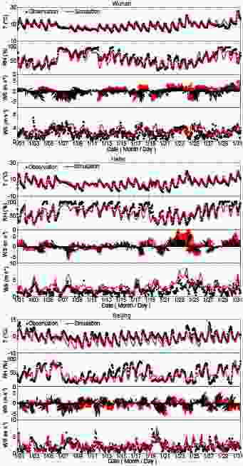 FigureS2. Temporal variation of the hourly simulated and observed Temperature (T), relative humidity (RH), wind direction, and wind speed (WS) at Wuhan and its surrounding cities including Changsha in Hunan Province, Hefei in Anhui Province, and Beijing. The black dots and red lines represent observed and simulated data, respectively.
Figure 2 displays the simulated monthly average concentrations of PM2.5 over Central and East China and the observed PM2.5 concentrations in 117 cities during January 2014. As shown by the observations and simulations, PM2.5 values over 150 μg m?3 were mainly distributed across the south of the NCP region, Central China, north of SouthC, and the Sichuan Basin. The average PM2.5 concentrations in January 2014 over the typical cities in the SouthC region (e.g., Changsha, Nanchang, Guangzhou), at 93.1 μg m?3 to 153.9 μg m?3, were relatively higher than those over the typical cities in the NCP region (e.g., Beijing, Tianjin, Shijiazhuang, Jinan, Zhengzhou), at 93.5 μg m?3 to 138.4 μg m?3. The model showed good performance for the magnitude and spatial distribution of PM2.5 concentrations over Central and East China. Figure 3 compares the hourly simulated and observed PM2.5 concentrations in Wuhan and the 15 provincial capital cities, with corresponding statistical parameters shown in Table S1. The simulated PM2.5 values were consistent with observations in most cities, with r values of approximately 0.48–0.73 and MBs within ±20 μg m?3, specifically for periods with sharp increases and decreases of the PM2.5 concentrations over the NCP, including Beijing, Tianjin, Shijiazhuang, Jinan, and Zhengzhou, as well as East China, including Shanghai, Hangzhou, and Nanjing. The mean fraction biases (MFBs) of ?10.5% to 22.6% and mean fraction errors (MFEs) of 31.6%–54.2% in all cities also suggest a good performance of NAQPMS, based on a previous study of the evaluation of PM simulation with chemical transport models (Boylan and Russell, 2006). Therefore, the high-precision simulated data of the PM2.5 concentrations served as a good basis for analyzing the variations in the spatiotemporal distributions of the PM2.5 pollution and quantifying the impacts of regional transport to the haze formation in Wuhan.
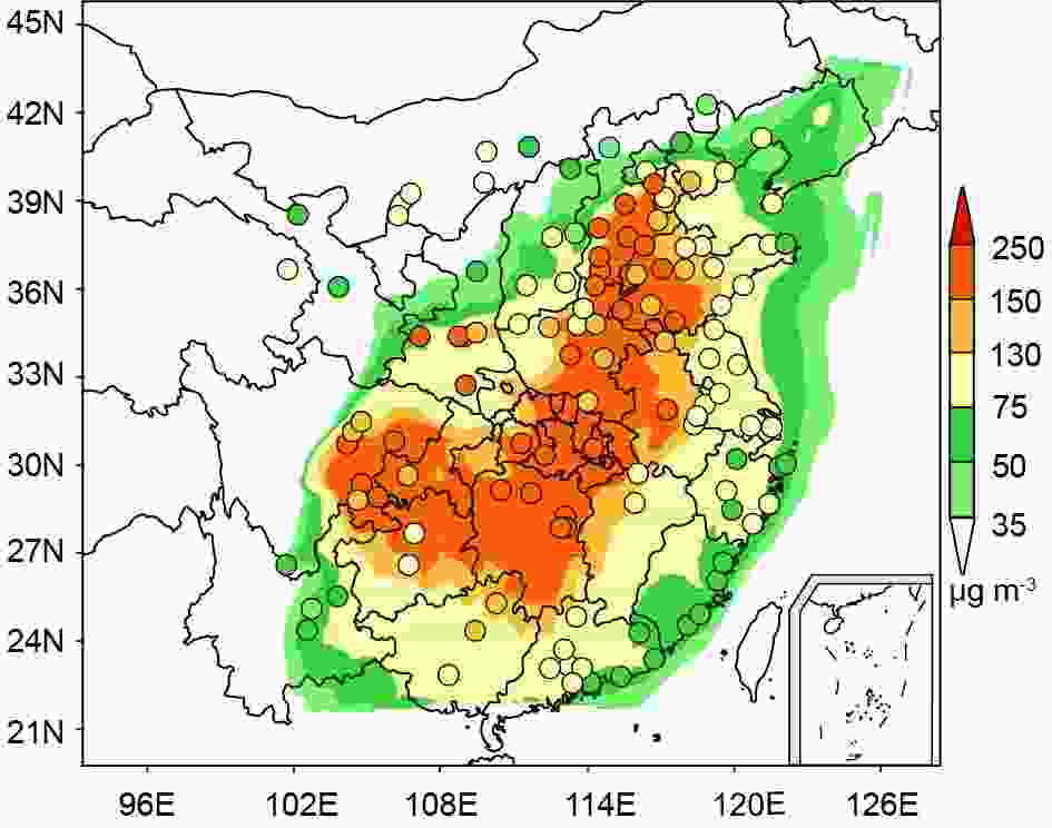 Figure2. The monthly mean concentrations of simulated PM2.5 (background color) and the observed values of 117 cities (solid circles) in the first modeling domain in January 2014.
 Figure3. Comparison between the hourly observed and simulated PM2.5 concentrations in Wuhan and the surrounding 15 capital cities over Central and East China. The red lines with open circles and black lines represent simulated and observed data, respectively.
| Number | Site | MO (μg m?3) | MM (μg m?3) | MB (μg m?3) | r | MFB (%) | MFE (%) |
| 1 | Beijing | 93.5 | 95.6 | 2.1 | 0.70 | 4.9 | 54.2 |
| 2 | Nanchang | 109.2 | 137.6 | 28.4 | 0.48 | 22.6 | 40.2 |
| 3 | Tianjin | 120.2 | 133.3 | 13.2 | 0.71 | 1.1 | 46.1 |
| 4 | Hefei | 155.5 | 159.6 | 4.1 | 0.71 | 1.7 | 31.6 |
| 5 | Shijiazhuang | 126.3 | 136.5 | 10.1 | 0.59 | 9.3 | 47.9 |
| 6 | Nanjing | 124.7 | 123.2 | ?1.5 | 0.69 | ?7.2 | 36.4 |
| 7 | Jinan | 130.7 | 148.4 | 17.7 | 0.70 | 14.6 | 42.5 |
| 8 | Shanghai | 89.6 | 101.8 | 12.2 | 0.73 | 6.5 | 51.8 |
| 9 | Zhengzhou | 138.4 | 157.1 | 18.7 | 0.63 | 7.2 | 38.4 |
| 10 | Hangzhou | 109.7 | 104.9 | ?4.8 | 0.70 | ?4.2 | 36.2 |
| 11 | Wuhan | 172.9 | 181.5 | 8.6 | 0.56 | 3.2 | 33.6 |
| 12 | Guangzhou | 93.1 | 96.8 | 3.7 | 0.27 | 1.1 | 44.8 |
| 13 | Changsha | 153.9 | 166.5 | 12.6 | 0.59 | 5.2 | 37.6 |
| 14 | Chengdu | 181.5 | 161.1 | ?20.5 | 0.52 | ?10.5 | 35.4 |
| 15 | Xi’an | 151.6 | 147.4 | ?4.2 | 0.63 | 9.1 | 41.4 |
| 16 | Taiyuan | 95.0 | 110.6 | 15.6 | 0.48 | 21.7 | 50.4 |
TableS1. Statistical parameters of the simulated and observed PM2.5 concentrations in Wuhan and its surrounding 15 capital cities over Central and East China in January 2014. The definitions of the abbreviations MO, MM, MB, r, MFB and MFE are provided below (Text S1).
2
3.2. Overall characteristics of meteorological conditions and haze episodes in Wuhan
Wuhan experienced a persistent haze pollution period for nearly the entire month of January 2014, which was significantly longer than that in Beijing with 18 polluted days. A detailed comparison of several statistics of the PM2.5 concentrations and the corresponding meteorological variables observed in Wuhan and Beijing during this period is shown in Table 2. The number of severely polluted days with a daily PM2.5 average ≥150 μg m?3 was 19, which was far more than that of Beijing at 4 days. The monthly average PM2.5 concentration reached 172.8 μg m?3 in Wuhan—almost twice as much as the 94.6 μg m?3 found in Beijing during January 2014, and much higher than the 121.0 μg m?3 also reported in Beijing during January 2013 (Zheng et al., 2015b). These results suggest that the haze pollution in Wuhan was far worse and persisted for a longer period compared to Beijing during January 2014.| Wuhan | Beijing | |
| Mean value | 172.8 μg m?3 | 94.6 μg m?3 |
| Polluted days | 30 days | 18 days |
| Peak PM2.5 | 347.0 μg m?3 | 538.0 μg m?3 |
| Daily increase | 116.8 μg m?3 d?1 | 215.6 μg m?3 d?1 |
| Hourly increase | 103.0 μg m?3 h?1 | 230.0 μg m?3 h?1 |
| Daily decrease | ?132.6 μg m?3 d?1 | ?242.9 μg m?3 d?1 |
| Hourly decrease | ?91 μg m?3 h?1 | ?192 μg m?3 h?1 |
| Non-haze days | 1 day (72.0 μg m?3) | 13 days (38.4 μg m?3) |
| Slightly polluted | 5 days (95.2 μg m?3) | 7 days (95.6 μg m?3) |
| Moderately polluted | 6 days (133.1 μg m?3) | 7 days (126.0 μg m?3) |
| Heavily polluted | 19 days (233.5 μg m?3) | 4 days (270.2 μg m?3) |
| T | 7.8°C | ?0.3°C |
| RH | 58.4% | 44.3% |
| WS | 2.4 m s?1 | 2.0 m s?1 |
Table2. General information on the PM2.5 concentration and corresponding meteorological elements in Wuhan and Beijing in January 2014. The days with daily PM2.5 concentrations over 75 μg m?3, 115 μg m?3, and 150 μg m?3 are defined as slightly, moderately, and heavily polluted days, respectively.
In view of the temporal variation in the PM2.5 values in Fig. 4, the daily values showed cyclic variations lasting approximately 4–10 days in Wuhan and approximately 3–7 days in Beijing. During the processes of accumulation among pollutants, the maximum rates of increase in the PM2.5 concentrations within one day and one hour in Wuhan were 116.8 μg m?3 d?1 and 103.0 μg m?3 h?1, respectively—much lower than the corresponding values of 215.6 μg m?3 d?1 and 230.0 μg m?3 h?1 in Beijing. The peak value of the hourly PM2.5 concentrations in Wuhan was 347.0 μg m?3 and occurred at 0800 LST 27 January, which was much lower than the observed peak value of 538.0 μg m?3 in Beijing. Additionally, the rates of decrease in the PM2.5 concentrations within one day and one hour in Wuhan were ?132.6 μg m?3 d?1 and ?91 μg m?3 h?1, approximately half the values of ?242.9 μg m?3 d?1 and ?192 μg m?3 h?1 in Beijing during the stages of decreasing PM2.5 concentrations. Wuhan’s minimum daily PM2.5 concentration was 72.0 μg m?3 in January, while it was only 9 μg m?3 in Beijing. The result suggests that the fluctuation of PM2.5 concentrations in Wuhan was much less than that in Beijing in January 2014.
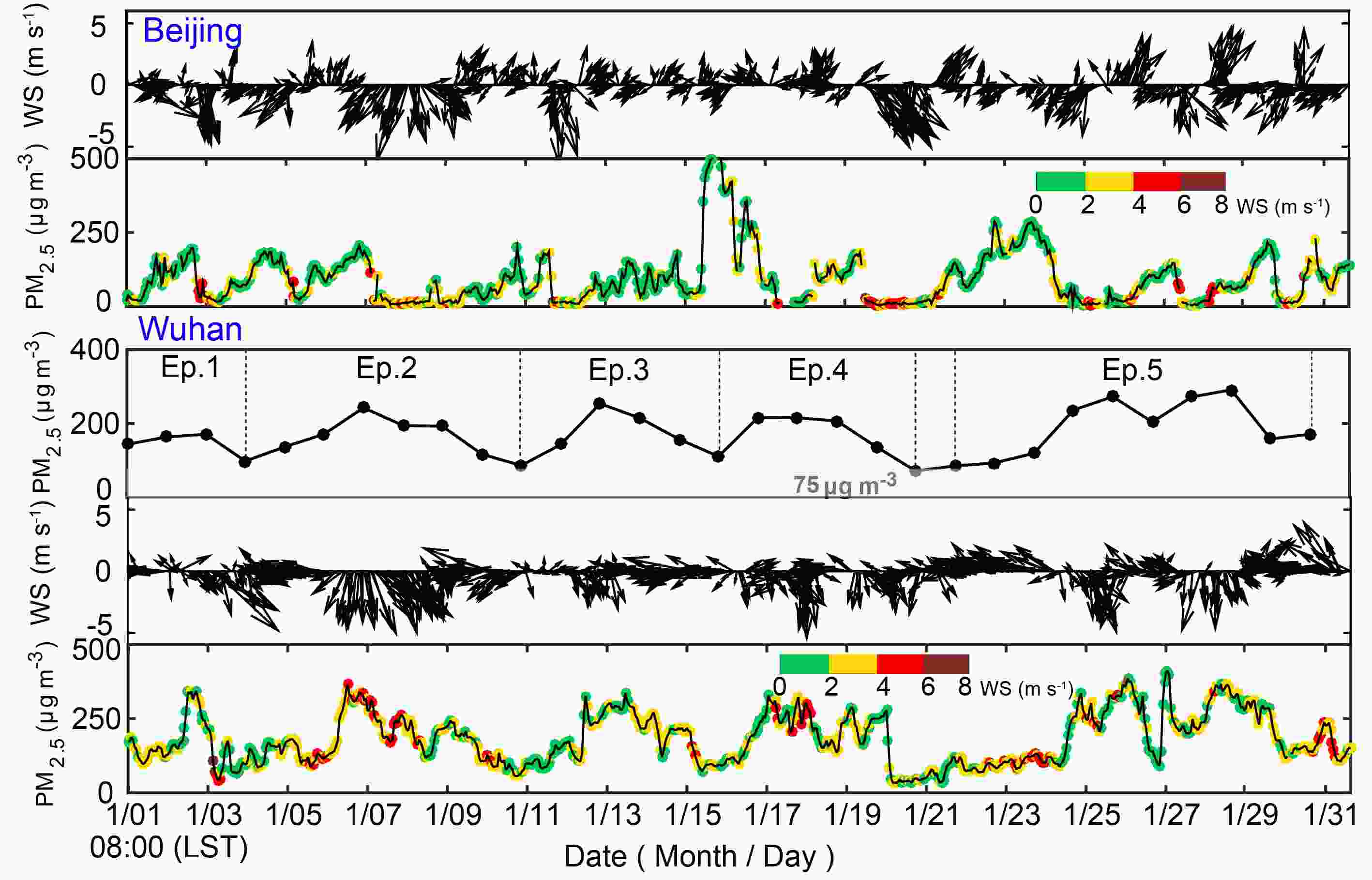 Figure4. The temporal variation in the observed hourly wind field and PM2.5 concentrations in Beijing and Wuhan in January 2014; the color represents the wind speed (WS). Five haze episodes were defined as Ep. 1–Ep. 5 based on the daily variation in the PM2.5 concentrations in Wuhan.
For a more detailed analysis, the haze pollution in January 2014 was divided into five episodes (Ep. 1–Ep. 5), shown in Table 3, based on the periodical variations of the daily PM2.5 concentrations, and we defined the sharp increasing and slow decreasing stages of PM2.5 concentrations as the early and later stages of the five episodes, except Ep. 5a and Ep. 5b (two special processes). As can be seen from Fig. 4, the sharp increases in the PM2.5 concentrations over Beijing were often accompanied by southerlies with low WSs of < 2 m s?1, and the rapid decreases in the PM2.5 concentrations corresponded to strong northerly winds. However, quite a different behavior was found for the relationship between the PM2.5 concentrations and the winds in Wuhan. The rapid increases in the PM2.5 values and the occurrence of the peak values in Wuhan were strongly associated with strong northerly winds. The above results suggest that the characteristics of the PM2.5 pollution (the change cycle, fluctuation amplitude, and relationship with winds) in Wuhan were distinct from those in Beijing in January 2014.
| Concentration Contribution | ||||||||
| Ep. | Stage | WS | Wuhan | AdjCity | NCP | EastC | SouthC | Others |
| Ep. 1 | early (1/1–1/3) | 2.3 | 58.0 | 48.7 | 13.3 | 1.8 | 36.4 | 39.3 |
| later (1/4) | 1.4 | 59.2 | 9.4 | 24.3 | 0.0 | 0.0 | 8.0 | |
| Ep. 2 | early (1/5–1/8) | 3.3 | 38.3 | 49.3 | 66.0 | 38.2 | 9.2 | 10.5 |
| later (1/9–1/11) | 2.1 | 69.1 | 33.0 | 7.8 | 10.8 | 0.2 | 0.5 | |
| Ep. 3 | early (1/12–1/13) | 1.6 | 55.6 | 24.9 | 94.9 | 10.8 | 0.0 | 15.7 |
| later (1/14–1/16) | 2.4 | 58.6 | 60.5 | 3.1 | 30.8 | 2.3 | 1.4 | |
| Ep. 4 | early (1/17–1/19) | 2.4 | 37.8 | 43.7 | 105.1 | 28.3 | 3.6 | 32.0 |
| later (1/20) | 1.9 | 19.8 | 9.4 | 19.7 | 0.1 | 0.1 | 19.1 | |
| Ep. 5 | early (1/25) | 2.5 | 26.2 | 17.7 | 182.1 | 8.2 | 16.3 | 38.1 |
| later (1/26–1/29) | 2.1 | 65.4 | 55.9 | 16.5 | 18.3 | 9.6 | 21.8 | |
| Ep. 5a (1/22–1/24) | 3.0 | 30.9 | 41.6 | 2.2 | 15.3 | 43.3 | 2.6 | |
| Ep. 5b (1/30–1/31) | 2.9 | 48.9 | 57.0 | 3.5 | 1.1 | 53.1 | 9.2 | |
Table3. The mean wind speed (WS, m s?1) and concentration contribution (μg m?3) of the PM2.5 concentrations over Wuhan from the local, nearby cities (AdjCity), North China Plain (NCP), East China (EastC), South China (SouthC), and other regions (Others) during different stages of the five haze episodes (Ep.) in Wuhan.
To further explore the influence of the planetary boundary layer structure on the PM2.5 pollution, Fig. 5 displays the evolution of the simulated horizontal wind, potential temperature, RH in the vertical direction, and the PBLH in Wuhan. As can be seen, the variation of the peak value of the daily PBLH was strongly consistent with thermal stratification during the entire study period, except for Ep. 5a and Ep. 5b, which indicated that the strong thermal stratifications suppressed the development of the PBLH. Also, in Ep. 5a and Ep. 5b, different source regions of air masses driven by the prevailing southerly winds may have been responsible for the strong thermal stratifications with high PBLH. Besides, higher daily maximum PBLH tended to occur during the build-up stages of the PM2.5 pollution, except for Ep. 2, which was almost opposite to the finding in Miao et al. (2019). The PBLH often decreased during the later stages of PM2.5 episodes, which would not have been favorable for the vertical dispersion of air masses and would have led to the local accumulation of air pollutants. Furthermore, Wuhan was influenced by strong northerly winds from the surface layer to the upper layer (at least 2000 m) during the stages of increasing PM2.5 concentrations, and there were relatively weak WSs with WDs shifting rapidly during the stages of decreasing PM2.5 concentrations. High PBLH and strong winds are often considered to be conducive to the diffusion of the air pollutants, which further illustrates the special features of the haze episodes that occurred in Wuhan during January 2014.
 Figure5. The vertical distribution of the simulated planetary boundary layer height (PBLH), potential temperature (θ), horizontal winds (V), relative humidity (RH), and PM2.5 concentrations in the vertical direction over Wuhan in January 2014.
Based on the sea-level weather patterns from the simulation data (see Fig. 6) and the corresponding synoptic weather maps of the Korea Meteorological Administration (see Fig. S3), the impact of the large-scale atmospheric circulation conditions on the formation of the PM2.5 pollution in Wuhan was investigated. Overall, there were two types of weather patterns leading to the increase of the PM2.5 concentrations in Wuhan.
 Figure6. The simulated sea-level weather patterns and wind fields at (a) 1500 LST 2 January 2014 (Ep. 1), (b) 2100 LST 7 January 2014 (Ep. 2), (c) 1400 LST 12 January 2014 (Ep. 3), (d) 2200 LST 16 January 2014 (Ep. 4), and (e) 1900 LST 24 January 2014 (Ep. 5).
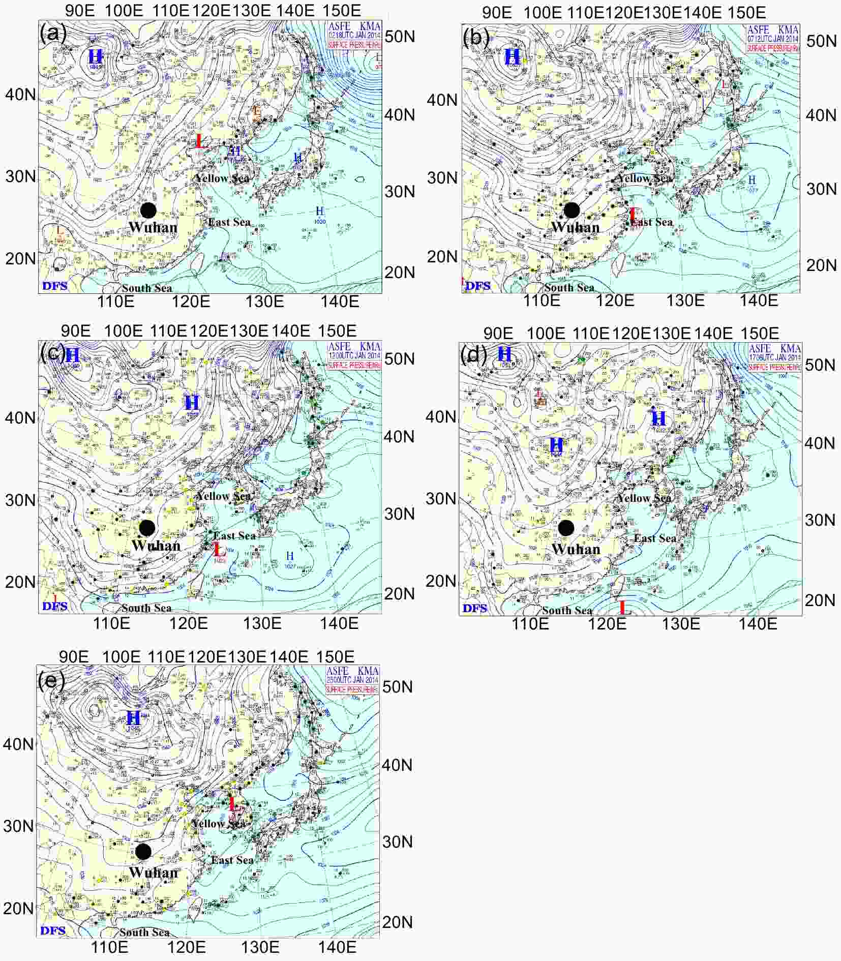 FigureS3. Sea-level weather pattern over eastern China at (a) 0200 LST 3 January 2014 (Ep. 1), (b) 2000 LST 7 January 2014 (Ep. 2), (c) 0800 LST 12 January (Ep. 3), (d) 1400 LST 17 January (Ep. 4), and (e) 0800 LST 25 January (Ep. 5) from the synoptic weather maps of the Korea Meteorological Administration.
Firstly, northerly winds were observed over Wuhan in the early stages of all haze episodes (Fig. 4), so we first analyzed the characteristics of weather patterns in upstream regions, including the whole of Central and East China and coastal areas in China (Fig. S3). It was found that a very similar configuration of the atmospheric circulation conditions over East Asia occurred in the early stages of Ep. 1–Ep. 2 and Ep. 5. Taking Ep. 2 for example, a strong and cold anticyclone from Mongolia moved southward, accompanied by a cyclonic system stagnating over the East China Sea. Such a configuration of weather systems led to a large pressure gradient and prevailing northerly winds over Central and East China. According to the observations in Fig. 4, the daily WS of 1.2 m s?1 on 6 January in Beijing increased to 2.3 m s?1 on 7 January, and the average value in Wuhan reached approximately 3.3–3.7 m s?1. During this period, Beijing experienced haze pollution, with observed daily mean PM2.5 values of 124.7 μg m?3 and 104.6 μg m?3 on 6 and 7 January, respectively. The strong northerly winds brought clean air masses from Mongolia to the NCP region, resulting in a significant decrease in the PM2.5 concentrations on 8 January (daily PM2.5 concentrations of 14.7 μg m?3 in Beijing). Simultaneously, the high concentrations of air pollutants over Beijing moved southward under the influence of the regional northerly winds, which were probably related to the rapid increase in the PM2.5 concentrations in Wuhan. Though the locations of the cyclonic and anticyclonic systems were slightly different, prevailing northwesterly winds in the northwest of the NCP and northerly winds in the NCP occurred during the stages of rapidly increasing PM2.5 concentrations in Ep. 1 and Ep. 5, respectively. In Ep. 3 and Ep. 4, a high-pressure system moving southeast was blocked by the strong weather system downstream and would have similarly resulted in strong winds over the NCP. Wuhan was in front of the surface high in Ep. 2 and Ep. 3, or controlled by sparse isobars in Ep. 1, Ep. 4 and Ep. 5, as shown in Fig. 6. Overall, the blocking high-pressure system moving southeastward was the key and typical weather pattern in the formation of the strong northerly winds in the NCP, and then the long-range transport of the polluted air masses from the NCP to Wuhan area.
The other type of atmospheric circulation controlled SouthCand Central China and occurred in Ep. 5a and Ep. 5b (see Fig. S4). The low-pressure system was located in Southwest China, and the high-pressure system was in the East China Sea. Such a configuration of two strong weather systems would have resulted in a large pressure gradient and prevailing southerly air flows over SouthC and Central China. According to the observations, persistent southerly winds dominated Wuhan, with average WSs of 3.0 m s?1 and 2.9 m s?1 in Ep. 5a and Ep. 5b, respectively.
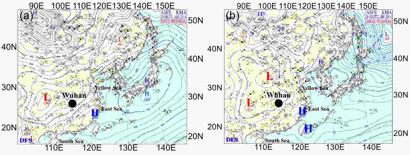 FigureS4. Sea-level weather pattern over eastern China at (a) 0200 LST 24 January 2014 and (b) 1100 LST 31 January 2014 from the synoptic weather maps of the Korea Meteorological Administration.
The results highlight two typical configurations of the synoptic systems related to Wuhan’s increase in PM2.5 concentrations and a strong link between the severe haze pollution over Wuhan in January 2014 to the regional haze pollution over the NCP and SouthC. This finding also indicates that special attention should be paid to the above configurations of synoptic systems and concurrent regional haze pollution over the NCP and SouthC with regards to the forecasting and control of haze pollution in Wuhan.
2
3.3. Mechanism for the formation and dissipation of PM2.5 episodes in Wuhan
The high-precision simulation data of the PM2.5 concentrations were used to investigate the formation and dissipation mechanism of the haze episodes in Wuhan.3
3.3.1. Mechanism for the sharp increase in PM2.5 concentrations
Figure 6 shows the distribution of simulated PM2.5 concentrations and winds during the sharp increase in PM2.5 concentrations in Ep. 1–Ep. 5. Taking Ep. 2 as an example, before the occurrence of the first synoptic system configuration mentioned in section 3.2, the NCP region, with the highest emission intensity of air pollutants in China, was suffering from regional haze pollution due to adverse meteorological conditions. A weak low-pressure band (not shown here) was the synoptic flow pattern associated with the occurrence of the haze episodes over the NCP region during January 2014. The weak WS, high RH, and shallow PBLH under this typical synoptic condition frequently leads to low-visibility events in winter (Ye et al., 2015). In addition, high RH provides favorable conditions for the hygroscopic growth of particles (Eichler et al., 2008), and aqueous or heterogeneous reactions of gaseous pollutants such as SO2 and NOx (Xie et al., 2015) that lead to significant increases in secondary pollutants in the NCP. As shown in Fig. 7b, the polluted air masses in NCP were transported to the Wuhan area when the northerly winds moved towards the south quickly. Video S1 and video S2 in the Electronic Supplementary Material provide detailed information on the evolution of the regional PM2.5 concentrations and wind fields in the horizontal and vertical directions during 6–8 January. As for the other episodes, similar pollutant transport processes are displayed in Figs. 7a, c, d and e. It should be noted that mountains, with a maximum altitude of 1777 m, are located in the north of the Wuhan city-cluster. In this case, the simulation results suggest that the air pollutants over the NCP can be transported directly to Wuhan due to the impetus of the strong weather system with high WSs. A different influence of the mountains on pollutant transport has been reported. In some cases with relatively weak northerly winds, the highest mountain peak in the north of the Wuhan city-cluster tends to change the transport pathway of the polluted air mass to a northwest or northeast route (Zhou et al., 2016; Bai et al., 2018).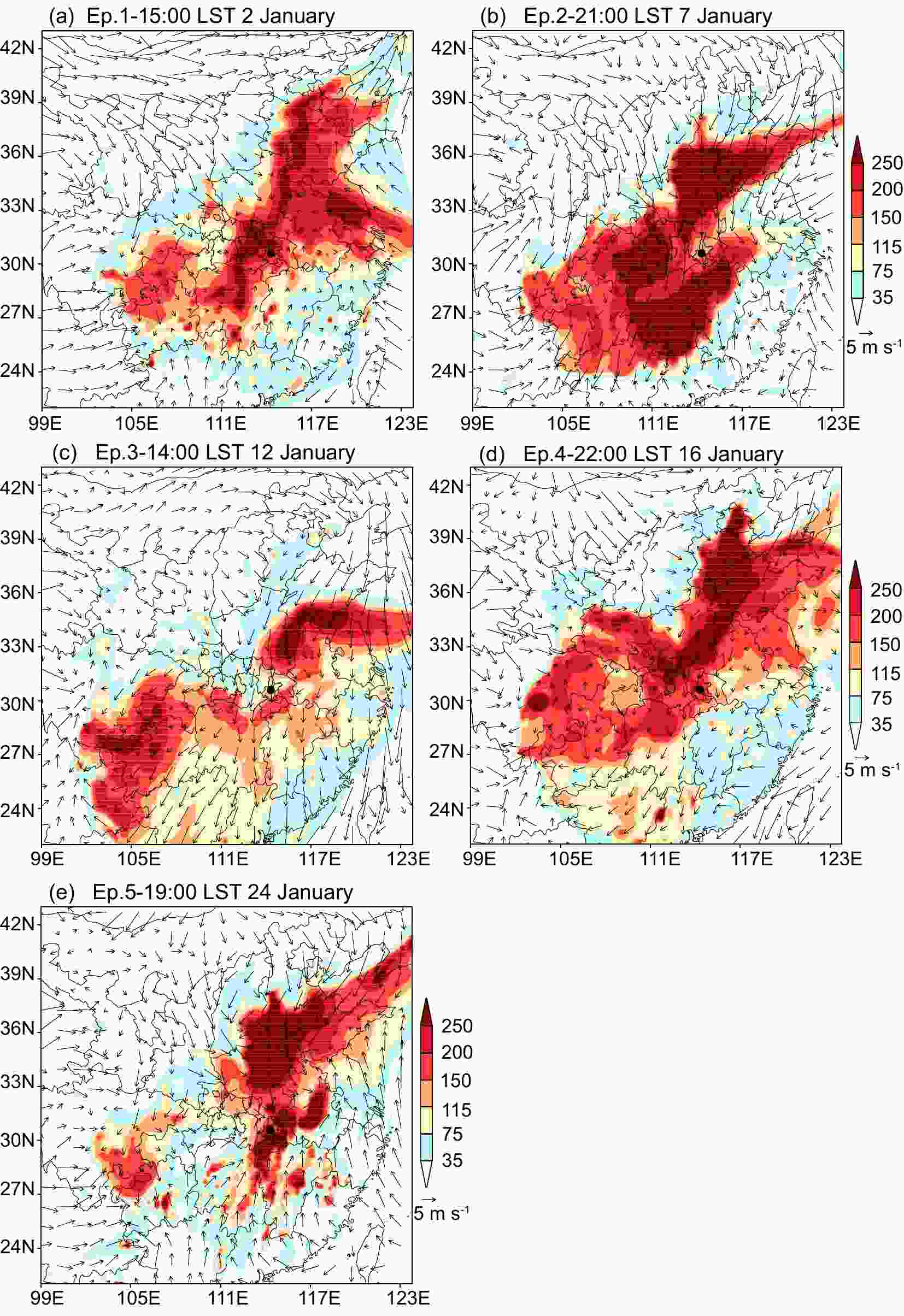 Figure7. The distribution of simulated PM2.5 concentrations (units: μg m?3) and winds at the same time as Fig. 6 during stages of increasing PM2.5 concentrations in Ep. 1–Ep. 5 over Wuhan in the first modeling domain.
To further identify the key source region contributing to Wuhan’s rapid increase in PM2.5 concentrations during January 2014, the source-tagged method described in section 2.2 was conducted. As shown in Fig. 1, the entire model domain was divided into six source regions based on administrative boundaries, including Wuhan, surrounding cities of Wuhan, the NCP, EastC, SouthC, and “AdjCity”. Figure 8 and Table 3 display the daily contributions of the six source regions to the PM2.5 concentration levels in Wuhan. During the early stage of the five episodes, the contribution rates from long-range regional transport were approximately 49.7%–84.9%, and the concentration contributions of PM2.5 reached approximately 90.8–244.7 μg m?3, with a mean value of 150.0 μg m?3. On the other hand, the contribution from local emissions was < 75 μg m?3 during the same period. This result suggests that long-range regional transport was the main factor for Wuhan’s rapid increase in PM2.5 concentrations, and was the direct trigger of the build-up of severe haze pollution in Wuhan during January 2014.
 Figure8. The observed daily average concentrations (black dotted lines) and mean contribution rate (column diagram) of PM2.5 over Wuhan among local, nearby cities (AdjCity), the North China Plain (NCP), East China (EastC), South China (SouthC), and other regions (Others).
From Fig. 8 and Table 3 we can see that the NCP was the most important source region. The average contribution of the NCP region to the PM2.5 concentrations in Wuhan reached 38.3% and 92.3 μg m?3 during the stages with rapidly increasing PM2.5 concentrations in the five episodes—especially Ep. 4 and Ep. 5, which showed concentration contributions of 105.1 μg m?3 and 182.1 μg m?3, respectively. If the contributions from the NCP were removed, the numbers of moderate and heavy pollution days in Wuhan during January 2014 were reduced by 4 days and 9 days, respectively. This result highlights the important impact of regional haze pollution over the NCP on the formation of haze episodes in Wuhan. Special attention should be paid to the NCP region with regards to mitigating and controlling haze pollution on a nationwide scale.
3
3.3.2. Mechanism for the slow decrease in PM2.5 concentrations
As described in section 3.2, the rates of decrease in PM2.5 concentrations in Wuhan in the five episodes were much slower than those observed in Beijing. This phenomenon was a key factor for connecting the five episodes to forming the haze pollution lasting almost an entire month in Wuhan. We investigated the characteristics of the meteorological conditions during the later stages. Figures 9a and c and 10a and c show the spatial distributions of the sea level pressure, wind fields and PM2.5 values. There were mainly two types of circulation fields found to be favorable to the decrease in the PM2.5 concentrations during the five episodes over Wuhan.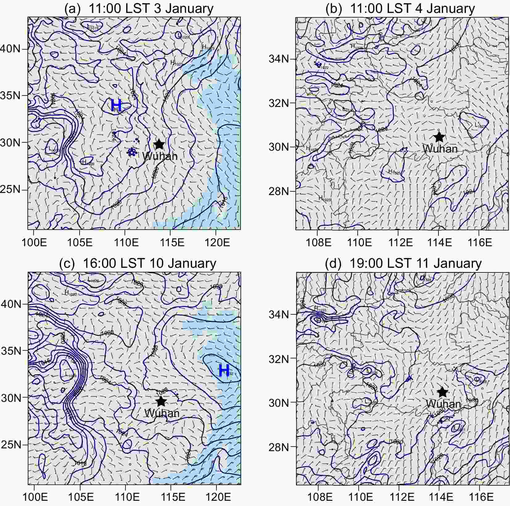 Figure9. The simulated sea-level weather patterns and wind fields at (a) 1100 LST 3 January in the first modeling domain (D1), (b) 1100 LST 4 January in the second modeling domain (D2), (c) 1600 LST 10 January in D1, and (d) 1900 LST 11 January in D2.
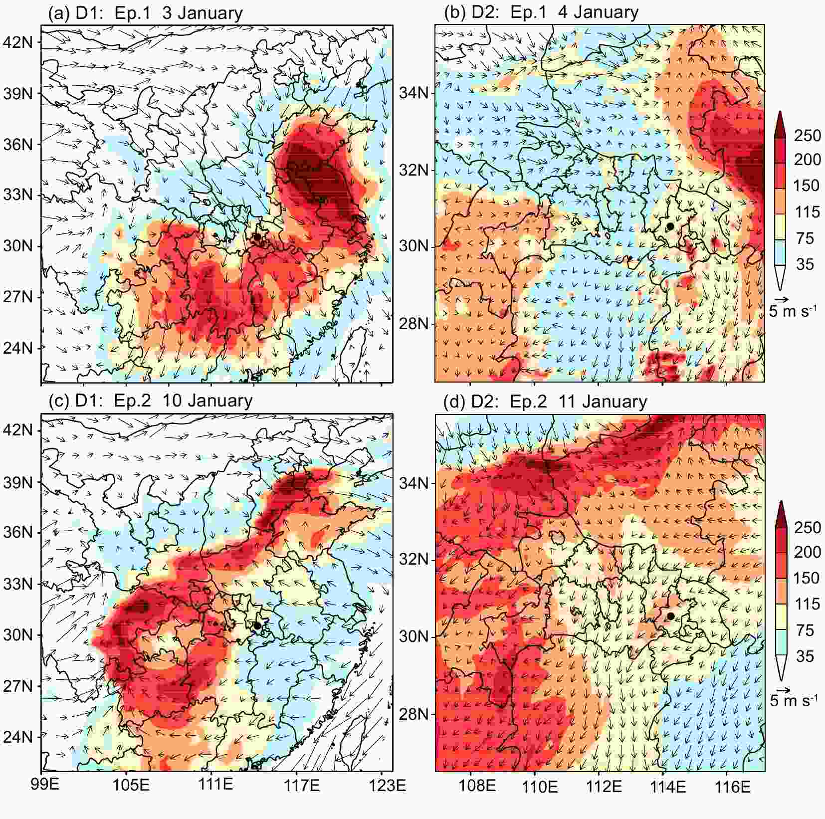 Figure10. The distribution of average simulated PM2.5 concentrations (units: μg m?3) and winds during the last two days of the haze episodes on (a) 3 January in the first modeling domain (D1) and (b) 4 January in the second modeling domain (D2) of episode 1 (Ep. 1), and (c) 10 January in D1 and 11 January in D2 of episode 2 (Ep. 2). The black dots represent Wuhan.
One situation, occurring in Ep. 1 and Ep. 4, was that prevailing northerly winds that dominated the whole of Central and East China with a strong high-pressure system from Siberia and Mongolia area moving southeastward. With the dry and clean air toward Wuhan, air pollutants dispersed partly. Ye et al. (2015) found that this typical atmospheric circulation reduces pollutant concentrations effectively over Beijing at the leading edge of the northerly cold advection in wintertime. Figure 4 also shows a similar situation in which the hourly PM2.5 concentrations in Beijing experienced a sharp decrease from 205 μg m?3 to 18 μg m?3 within 8 h and remained at values lower than 20 μg m?3 under the influence of northerly winds with daily WSs of approximately 2.3–3.5 m s?1 on 7 and 8 January. The second situation, occurring in Ep. 2, Ep. 3 and Ep. 5, was that a high-pressure system stagnated over eastern coastal areas of China and resultant regional easterly winds were conducive to removing the particle concentrations in Wuhan. This second typical situation is tightly linked to the mitigation of air pollution in EastC under the control of clean maritime airstreams (Shu et al., 2017). However, these two strong circulation fields did not lead to the expected decrease in Wuhan’s PM2.5 concentrations.
The main reason for the ineffectiveness of the two strong atmospheric conditions in removing pollutants from Wuhan was the city’s geographic limitations—specifically, the city being located in the center of regional haze pollution covering large areas of China (Fig. 2). When the clean air brought by the strong atmospheric circulation system was close to Wuhan, the circulation system often changed. As shown in Fig. 9, Wuhan was in front of the surface high on 3 January and was behind the offshore high-pressure system on 10 January, and then controlled by sparse isobars in the following days. The transitions of weather patterns were also found in the other episodes. Therefore, winds shifted from a northerly direction to a weak northeasterly one in Ep. 1, to a weak northeasterly one in Ep. 4, and to a weak southerly one in Ep. 5, respectively shown in Fig. 10 and Fig. S5. Additionally, prevailing easterly winds that were also carrying clean air weakened in Ep. 2 and Ep. 3. The results suggest that the change in the circulation system led to the end of the prevailing northerly winds and sea winds. By comparison, the high PM2.5 concentrations in Beijing could be eliminated immediately by the strong northerly winds due to its location at the edge of the regional haze (see Fig. 2) and lasted shorter (3–7 days) than that (4–10 days) in Wuhan. On the other hand, the variations of the PM2.5 concentrations of the two cities were strongly related under the influences of cold air from Siberia. From Fig. 5, the WS gradually decreased in the later stages of the episodes from the ground to a height of approximately 1.5 km, and the WDs shifted rapidly on the last day of the episodes on 4, 11, 16, 21 and 29 January. Referring to Ep. 2 as an example, the evolution of the PM2.5 pollution under weak winds is shown in Video S1 and Video S2. The stable weather conditions and weak winds were responsible for the accumulation of air pollutants and the maintenance of high PM2.5 concentrations in Wuhan during the later stages of the episodes. This would have been another key factor for the 30 haze days seen in Wuhan, as well as the long-range regional transport during the early stages of the episodes.
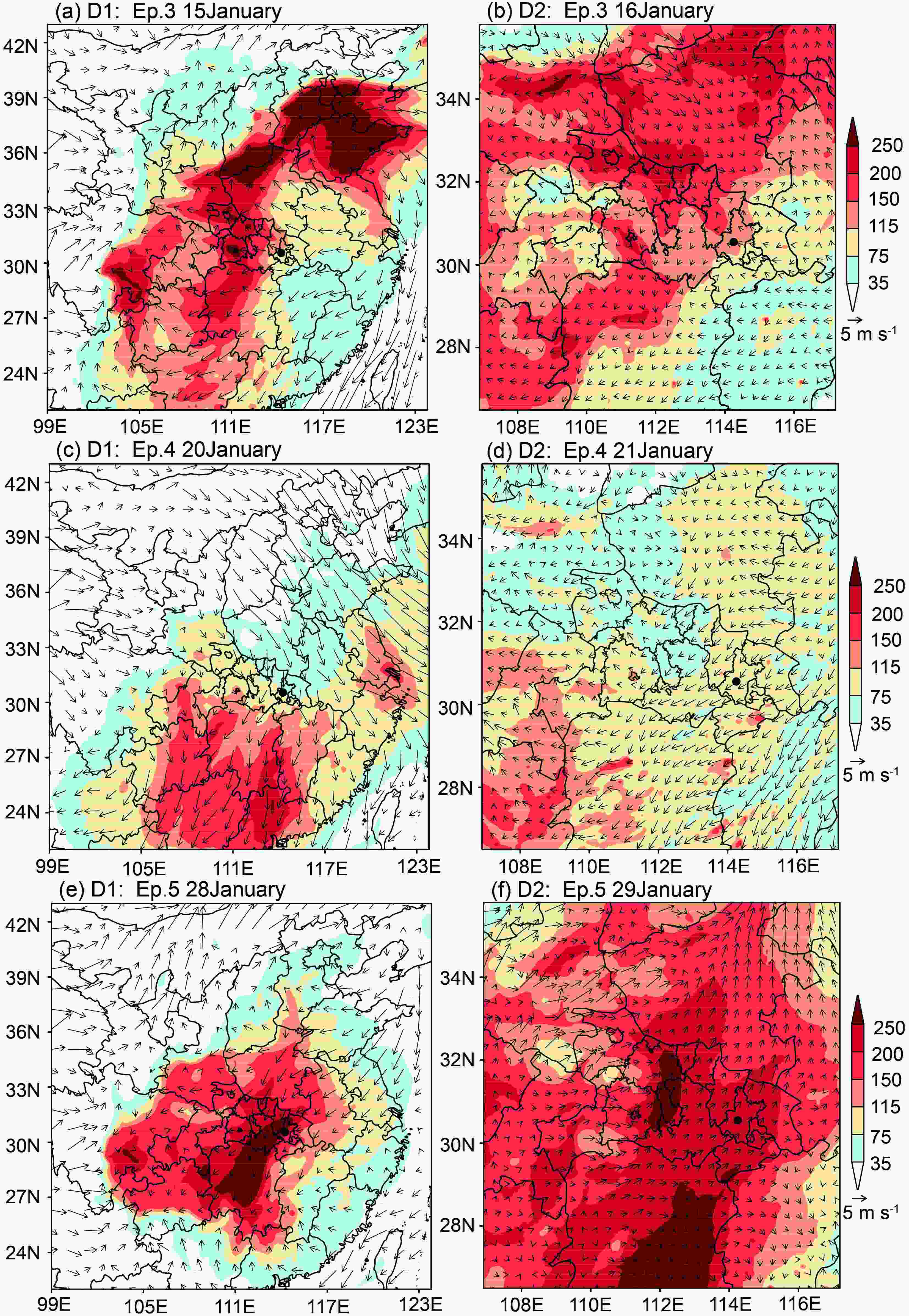 FigureS5. The distribution of the PM2.5 concentrations (units: μg m?3) and winds (units: m s?1) during the last two days of haze sub-episodes on (a) 15 January in the first modeling domain (D1) and (b) 16 January in the second modeling domain (D2) of sub-episode 3 (Ep.3); (c) 20 January in D1 and (d) 21 January in D2 of sub-episode 4 (Ep. 4); and (e) 28 January in D1 and (f) 29 January in D2 of sub-episode 5 (Ep. 5). The black dots represent Wuhan.
Additionally, there were a few cases that were not related to the regional transport of particles from the NCP, but rather to the transport from SouthC. As shown in Fig. 4, southerly and southeasterly winds occurred in Wuhan in Ep. 5 from 22 to 24 January (see Ep. 5a) and 30 and 31 January (see Ep. 5b), with daily average winds of approximately 2.6–3.6 m s?1 and 2.5–3.3 m s?1 and hourly peaks of 4.6 and 4.9 m s?1, respectively. According to the surface atmospheric circulation (Fig. S4), SouthC was controlled by a similar atmospheric circulation during these two periods. The low-pressure system was located in Southwest China, and the high-pressure system was in the East China Sea. Figures 5 and 11 show prevailing and persistent southerly winds were observed over SouthC and Wuhan from the ground to a height of 2.5 km. On 24 and 30 January, polluted air masses in SouthC with PM2.5 concentrations higher than 150 μg m?3 and 300 μg m?3, respectively, were transported to the Wuhan area by strong southerly winds. This further highlights the severity and complexity of PM2.5 pollution in Wuhan—especially pertaining to the city’s centrality among multiple city clusters. The variation in the PM2.5 pollution over Wuhan during the wintertime is strongly associated with the regional PM2.5 pollution over the extended areas of China, which makes pollution control in Wuhan more complex and difficult.
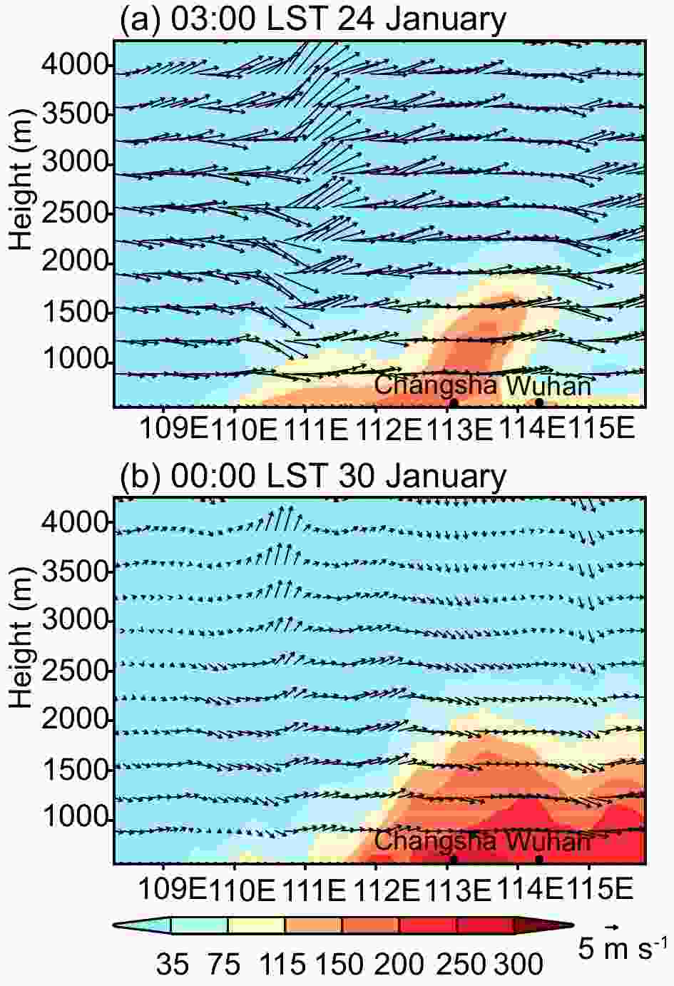 Figure11. The distribution of simulated PM2.5 concentrations (units: μg m?3) and wind fields in the vertical direction from South China to Wuhan via Changsha in Hunan Province at (a) 0300 LST 24 January and (b) 0000 LST 30 January.
Source-tagged modeling analyses were also conducted during the later stages of the five episodes. As shown in Fig. 8 and Table 3, the emissions from Wuhan and its surrounding cities contributed approximately 42.9%–84.8% of the PM2.5 concentrations during these periods, thus becoming the dominant sources of the PM2.5 pollution in Wuhan. In addition, the emissions from the NCP had important impacts on Wuhan’s PM2.5 concentrations during the later stages of Ep. 1 and Ep. 4, with average contributions of 24.1% and 29.0% respectively. Furthermore, the emissions from East China had an important influence during the later stages of Ep. 2 and Ep. 5, with average contributions of 21.0% and 10.7% respectively. Moreover, South China played a key role in the occurrence of haze days over Wuhan in Ep. 5a and Ep. 5b, contributing 30.3% and 31.8% of the PM2.5 concentrations respectively. The southern adjacent cities such as Xianning and Huangshi, contributed 31.1% and 33.0% with regional southerly winds. The contributions from local emissions were 30.9 μg m?3 and 48.9 μg m?3 or < 30%, respectively. The results above confirm the important roles played by the emissions from Wuhan and its surrounding cities in retaining high PM2.5 concentrations in Wuhan under weak winds and stable weather conditions during the later stages of the episodes. Both the high pollutant concentrations in source regions and the conducive wind field (e.g., relatively strong WS) are key factors in the occurrence of pollutant transport to Wuhan. Furthermore, the results also suggest that the haze pollution in Wuhan was aggravated by complex regional sources, including from the NCP, EastC and SouthC, and AdjCity. These key source regions could change rapidly with the meteorological conditions because of Wuhan’s location in the center of the regional haze pollution of China in that month. The change in the WD could only change the source regions of PM2.5 pollution in Wuhan, but it proved difficult to bring clean air quickly. Therefore, pollution control in Wuhan is a more complex issue compared to other regions, which raises concerns for rolling out effective national pollution control policies considering China’s diverse geography and regional climates.
(1) During the early stages of the five episodes, with a rapid increase in the PM2.5 concentrations, Wuhan, Central China and East China were dominated by strong northerly winds under a very similar synoptic system configuration. The strong northerly winds drove the polluted air masses past the NCP region to move further southward, leading to sharp increases in PM2.5 concentrations in Wuhan. The long-range transport was the main trigger for the formation of severe haze pollution during these stages, with contributions to the PM2.5 concentrations in Wuhan of approximately 49.7%–84.9%. The NCP was the key source region, with contributions of approximately 10.6%–63.0%.
(2) During the later stages of the five episodes, two atmospheric circulation conditions were favorable to the decreasing PM2.5 concentrations in Wuhan, but they did not lead to the expected decrease in PM2.5 concentrations to a healthy level like in Beijing. This was because Wuhan and Beijing were respectively located in the center and at the edge of where the regional haze pollution in Central and East China converged. Such a distribution of the regional haze made it difficult for the haze episodes in Wuhan to be dispersed by clean winds, and made them last longer than those in Beijing. Meanwhile, when the clean air brought by a strong synoptic system was close to Wuhan, the circulation system often changed and led to weakened winds and stable meteorological conditions over Central China. Therefore, the local accumulation of air pollutants over Wuhan and complex regional transport from surrounding cities, the NCP, EastC and SouthC occurred, which connected five episodes to form haze pollution of 30 days in January over Wuhan.
The results of this study highlight the special characteristics of the haze episodes in Wuhan during January 2014 and the strong relationship between the formation of PM2.5 pollution and regional transport from the NCP, EastC, SouthC, and AdjCity during the wintertime. It implies that applying interventions for pollution control in Wuhan is very complicated and raises challenges for national pollution control policies in China, as they must consider the environmental relations and geography. Further investigation of the air pollutant transport relationship between these regions would be useful for revealing the causes and formation of such extended haze pollution in China as shown in Fig. 2. In addition, considering the important role played by the emissions from the NCP in the build-up of the haze episodes in Wuhan, it would be important to see whether air quality improvement in the NCP (
In this study, some uncertainties—mainly from the methods employed—should be discussed. Firstly, the NAQPMS version without meteorology–aerosol feedback was used to simulate the pollution process over Wuhan in January 2014, which basically reproduced the spatial and temporal distribution of PM2.5 concentrations in 16 major capital cities across the country (see section 3.1 for more analysis). However, aerosol–meteorology interactions can change aerosol concentrations via physical mechanisms such as altering radiation budgets or cloud microphysical processes (Chen et al., 2014; Zhang et al., 2018), which may bring some uncertainties for the simulation results of the air quality model. Research by Zhang et al. (2018) showed that the enhancement of PM2.5 concentrations due to aerosol–radiation interactions was about 8.9 μg m?3 (6.9%) in January 2014, while the impact of cloud microphysics was very small. Numerical models with aerosol–meteorology interactions would require more thought in future research, which may reduce errors caused by the mechanism. In addition, the online source-tagged method employed in this study was considered as an efficient method for a range of source apportionment studies and has been widely used to quantify the regional contribution of PM, ozone, or other pollutants to a particular area. Compared to the traditional sensitivity method, such as the turning on/off of emissions, this method can effectively reduce errors caused by the nonlinearity of various chemical reactions among pollutants (He et al., 2008; Li et al., 2010). Moreover, online source apportionment has a relatively low computational cost because it can track the contribution of multiple source locations in one simulation. However, all molecules of a particular species have the same probability of reacting at a given time and location in the algorithm (Wagstrom et al., 2008). For example, SO2 emitted by power plants reacts identically to SO2 emitted by oil-refining facilities at a given time and grid. Such a hypothesis may give rise to a certain level of error in the calculation, which needs to be addressed in future studies.
Acknowledgments. The authors express their utmost gratitude to the NCAR for providing important biomass burning emissions data (FINNv1). We also thank Professor Shaodong XIE, Peking University, and Zhichao ZHU and Peipei QIU, Wuhan Research Academy of Environmental Sciences, for providing Wuhan’s 2014 emissions data. This study was supported by the National Key R&D Program (Grant Nos. 2017YFC0212603 and 2017YFC0212604), the Chinese Academy of Sciences Strategic Priority Research Program (Grant No. XDA19040201), and the National Natural Science Foundation of China (Grant Nos. 41575128 and 41620104008).
Open Access This article is distributed under the terms of the Creative Commons Attribution License which permits any use, distribution, and reproduction in any medium, provided the original author(s) and the source are credited.
Electronic supplementary material: Supplementary material is available in the online version of this article at
Electronic Supplementary Material to: Investigating the Transport Mechanism of PM2.5 Pollution during January 2014 in Wuhan, Central China*
Miaomiao LU1,2,6, Xiao TANG1,3, Zifa WANG1,3,6, Lin WU1, Xueshun CHEN1, Shengwen LIANG4, Hui ZHOU5, Huangjian WU1,6, Ke HU4, Longjiao SHEN4, Jia YU4, and Jiang ZHU1,6
1State Key Laboratory of Atmospheric Boundary Layer Physics and Atmospheric Chemistry,Institute of Atmospheric Physics, Chinese Academy of Sciences, Beijing 100029, China2State Environmental Protection Key Laboratory of Urban Ambient Air Particulate Matter Pollution Prevention andControl, College of Environmental Science and Engineering, Nankai University, Tianjin 300350, China3Center for Excellence in Regional Atmospheric Environment, Institute of Urban Environment,Chinese Academy of Sciences, Xiamen 361021, China4Wuhan Environmental Monitoring Center, Wuhan 430015, China5Hunan Meteorological Observatory, Changsha 410118, China6University of Chinese Academy of Sciences, Beijing 100049, China
ESM to: Lu, M. M., and Coauthors, 2019: Investigating the transport mechanism of PM2.5 pollution during January 2014 in Wuhan, Central China. Adv. Atmos. Sci., 36(11), 1217–1234, https://doi.org/10.1007/s00376-019-8260-5.
Text S1. Statistical parameters for model validation (“sim” and “obs” represent the simulated and the corresponding observed variables, respectively).
MO (mean observation)
MM (mean simulation)
MB (mean bias)
r (correlation coefficient)
MFB (mean fraction bias)
MFE (mean fraction error)
