Ming Li^,, Zi-Liang Cai, Zhi-Bo Feng, Zheng-Yin ZhaoCollege of Science, Xuchang University, Xuchang 461000, China

Received:2021-05-26Revised:2021-08-12Accepted:2021-08-16Online:2021-09-14


Abstract
Applying the transfer matrix and Green's function methods, we study the valley-resolved transport properties of zigzag graphene nanoribbon (ZGNR) junctions. The width of the left and right ZGNRs are N_L and N_R, and N_L ≥ N_R. The step/dip positions of the conductance G, the intravalley transmission coefficients (T_KK and ${T}_{{K}^{{\prime} }{K}^{{\prime} }}$), and the valley polarization efficiency ${P}_{{{KK}}^{{\prime} }}$ correspond to the subband edges of the right/left ZGNR that are controlled by N_R/N_L. The intervalley transmission coefficients (${T}_{{{KK}}^{{\prime} }}$ and ${T}_{{K}^{{\prime} }K}$) exhibit peaks at most of the subband edge of the left and right ZGNRs. In the bulk gap of the right ZGNR, ${T}_{{{KK}}^{{\prime} }}$ $={T}_{{K}^{{\prime} }K}$=0, and ${P}_{{{KK}}^{{\prime} }}$ = ±1, the valley polarization is well preserved. As N_R increases, the energy region for ${P}_{{{KK}}^{{\prime} }}$ = ±1 decreases. When N_L is fixed and N_R decreases, G, T_KK, ${T}_{{K}^{{\prime} }{K}^{{\prime} }}$ and ${P}_{{{KK}}^{{\prime} }}$ exhibit more and more dips, and the peaks of ${T}_{{{KK}}^{{\prime} }}$ (${T}_{{K}^{{\prime} }K}$) become more and more high, especially when (N_L − N_R)/2 is odd. These characters are quite useful for manipulating the valley dependent transport properties of carriers in ZGNR junctions by modulating N_L or N_R, and our results are helpful to the design of valleytronics based on ZGNR junctions.
Keywords： transfer matrix method;ZGNR junction;valley polarization;Landauer–Büttiker formula;edge state


PDF (2009KB)MetadataMetricsRelated articlesExportEndNote|Ris|BibtexFavorite
Cite this article
Ming Li, Zi-Liang Cai, Zhi-Bo Feng, Zheng-Yin Zhao. Valley-resolved transport in zigzag graphene nanoribbon junctions. Communications in Theoretical Physics, 2021, 73(11): 115701- doi:10.1088/1572-9494/ac1d9f

1. Introduction

With the progresses in fabricating stable graphene nanostructures, various electronic and optical properties of these structures, including graphene quantum dots, have been explored [1–3]. Since graphene has exceptional electron and thermal transport properties, it is a promising material that can be used in advanced low-energy electronic devices [4–7]. Zhang and Wu et al [8–10] investigated the resonant tunneling through S- and U-shaped graphene nanoribbons (GNRs) and graphene nanorings in between two semi-infinite zigzag GNR leads, thus tunability of the resonant tunneling is realized by only changing the geometry of the GNRs. Furthermore, a GNR junction can be formed by interconnecting two semi-infinite GNRs with different widths [11]. Moreover, the conductance of GNR metal–semiconductor junctions, as the key elements in all-graphene circuits, has been studied in detail recently [12–14]. Due to the energy mismatch between subbands in the left and right zigzag graphene nanoribbons (ZGNRs), a traveling carrier is scattered by the junction interface, which causes a finite junction conductance [11, 15, 16].

In addition to charge and spin, carriers in graphene host an extra valley degree of freedom, because there are two degenerate and inequivalent valleys (K and ${K}^{{\prime} }$) at the corners of the first Brillouin zone [17–19]. The valley-dependent properties in graphene have attracted a great amount of interest [7, 20–25]. A. Rycerz et al [21] proposed a valley filter and an electrostatically controlled valley valve based on a quantum point contact in a graphene sheet. Wu et al [25] showed that the gauge fields induced by strain can lead to valley-dependent transport phenomena in a single layer of graphene, such as the Brewster angles and the Goos–Hänchen effect. Other novel two-dimensional honeycomb lattice materials, such as silicene [26] and transition metal dichalcogenides [27] also have the valley degree of freedom. So the new field of valleytronics is born out of the manipulation of valley degree of freedom for carriers in these materials [20, 28–31].

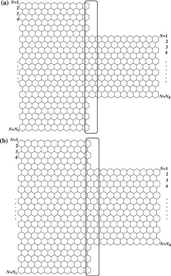
Moreover, to utilize the valley as an information carrier, the valley polarization efficiency of the transmission current is a key quantity. However, the valley degree of freedom is dependent on the momentum and highly related to the translation invariance of the crystal lattice. Therefore, for systems with interfaces, disorders as well as bias voltages, translational symmetry (TS) is broken and the momentum is not a good quantum number [32]. For systems lacking TS, the valley depolarization effect can be induced even without any disorder, which must be considered in the design of valleytronic devices [33]. It is therefore interesting to ask, what will the valley transport be like in a GNR junction? We wonder under such circumstances, whether the valley filter still perform high valley efficiency. What is more, modulation of the valley-resolved transport properties of ZGNR junctions by the width of the left and right ZGNRs has not been studied, which is crucial for designing valley filter with high efficiency based on ZGNR junctions. Thus in this paper, we main study ZGNR junctions. The left and right leads are composed of semi-infinite ZGNRs, and the central conduction region is marked by a box as shown in figure 1, which is different from that in [8–10, 21, 25]. By applying the transfer matrix and Green's function methods and analyzing the width dependent conductance channels (the edge states, the conduction subbands and valence subbands), we systematically investigate the dependence of valley-resolved transport properties of ZGNR junctions on the width of the left and right ZGNRs, and results are analyzed in detail. Step positions of G, T_KK, ${T}_{{K}^{{\prime} }{K}^{{\prime} }}$ and ${P}_{{{KK}}^{{\prime} }}$ are decided by N_R. As N_R increases, G, T_KK , ${T}_{{K}^{{\prime} }{K}^{{\prime} }}$ and their step numbers increase, the energy region for ${P}_{{{KK}}^{{\prime} }}=\pm 1$ decreases. For a fixed N_L and decreasing N_R, G, T_KK and ${T}_{{K}^{{\prime} }{K}^{{\prime} }}$ decrease, outside the bulk gap of the right ZGNR, G (T_KK, ${T}_{{K}^{{\prime} }{K}^{{\prime} }}$ and ${P}_{{{KK}}^{{\prime} }}$) exhibits more and more dips, and the peak values of ${T}_{{{KK}}^{{\prime} }}$ (${T}_{{K}^{{\prime} }K}$) become more and more large, especially when (N_L − N_R)/2 is odd. These transmission characters may be utilized to manipulate the valley degree of electrons in ZGNR junctions in the future.

Figure 1.

New window|Download| PPT slide
Figure 1.The geometry of ZGNR junctions. In the upper/lower panel, (N_L − N_R)/2 is even/odd. The central conduction region is marked by a box.


The rest of the paper is organized as follows. In section 2, we briefly introduce the transfer matrix and Green's function methods (the detailed descriptions are given in the appendix), the tight-binding model and the specific structure of ZGNR junctions. Results of numerical calculation and discussion are given in section 3. Finally, we give the conclusion in section 4.

2. Model and method

Figure 1 shows the geometry of ZGNR junctions, the left and right leads are composed of semi-infinite ZGNRs, and the central conduction region is marked by a box. Here N_L and N_R denote the width of the left and right ZGNRs, and N_L ≥ N_R. The Hamiltonian for the ZGNR junction reads [34–37](1)$\begin{eqnarray}H=-t\sum _{\langle {ij}\rangle \alpha }{c}_{i\alpha }^{\dagger }{c}_{j\alpha }.\end{eqnarray}$Here t = 2.75 eV is the transfer energy of the nearest neighbor hopping, ⟨ij⟩ represents the nearest neighbors. For ZGNR junctions, we assume that all edge sites at the interface are terminated by hydrogen atoms, and neglect the difference between the values of the site energy and the transfer energy for the atoms at the edge and the center [3, 38, 39].

Adopting the transfer matrix and Green's function method (see the appendix for detail), the physical transmission matrix element from mode (channel) i in the left terminal to mode (channel) j in the right terminal t_ij is calculated [32, 40–44]. The valley-resolved transmission coefficients are obtained by collecting t_ij in two separate valleys (K and ${K}^{{\prime} }$), and the transmission coefficient from valley K in the left terminal to valley ${K}^{{\prime} }$ in the right terminal is [32, 44](2)$\begin{eqnarray}{T}_{{{KK}}^{{\prime} }}(E)=\sum _{i\in K}\sum _{j\in {K}^{{\prime} }}{\left|{t}_{{ij}}(E)\right|}^{2}.\end{eqnarray}$

The linear conductance of the junction at zero temperature can be calculated by $G=\tfrac{2{e}^{2}}{h}({T}_{{KK}}+{T}_{{K}^{{\prime} }K}+{T}_{{{KK}}^{{\prime} }}\,+{T}_{{K}^{{\prime} }{K}^{{\prime} }})$ [45]. To investigate the valley polarization of transmission current, the valley polarization efficient is defined as [32](3)$\begin{eqnarray}{P}_{{{KK}}^{{\prime} }}=\displaystyle \frac{{T}_{{KK}}+{T}_{{K}^{{\prime} }K}-{T}_{{{KK}}^{{\prime} }}-{T}_{{K}^{{\prime} }{K}^{{\prime} }}}{{T}_{{KK}}+{T}_{{K}^{{\prime} }K}+{T}_{{{KK}}^{{\prime} }}+{T}_{{K}^{{\prime} }{K}^{{\prime} }}}.\end{eqnarray}$

3. Results and discussion

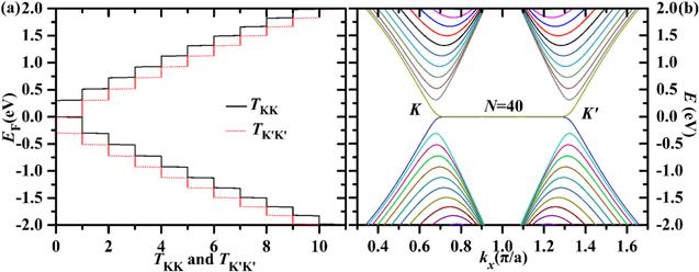
Figure 2 shows the intravalley transmission coefficients (T_KK and ${T}_{{K}^{{\prime} }{K}^{{\prime} }}$) as a function of E_F for a ZGNR with N_L = N_R = 40 and the corresponding energy band structure. Indeed, when E_F > 0, the step positions of T_KK and ${T}_{{K}^{{\prime} }{K}^{{\prime} }}$ coincide with the minima of the conduction subbands, while they coincide with the maxima of the valence subbands when E_F < 0. Therefore, the plateau height/step positions of T_KK and ${T}_{{K}^{{\prime} }{K}^{{\prime} }}$ are determined by the number/edges of occupied transverse subbands that are controlled by the ribbon width N. As can be seen in figures 2(a) and 2(b), ${T}_{{KK}}/{T}_{{K}^{{\prime} }{K}^{{\prime} }}$ jumps from 0 to 1 at E_F = 0, then increases step by step with decreasing/increasing E_F, and ${T}_{{KK}}/{T}_{{K}^{{\prime} }{K}^{{\prime} }}$ jumps from 0 to 1 when E_F crosses the lowest conduction subband/topmost valence subband, then increases step by step with increasing/decreasing E_F. In fact, this is also the case for G and ${P}_{{{KK}}^{{\prime} }}$, as shown in figure 3. Around E_F = 0, there are two conducting channels contributing to G by the edge states, but only the one at ${K}^{{\prime} }/K$ valley contributes to G when E_F > 0/E_F < 0, assuming the current is right-going in the device. Thus the carriers can transmit through the ${K}^{{\prime} }$ valley and ${T}_{{K}^{{\prime} }{K}^{{\prime} }}({E}_{F})\gt {T}_{{KK}}({E}_{F})$ when E_F > 0, and through the K valley and ${T}_{{K}^{{\prime} }{K}^{{\prime} }}({E}_{F})\lt {T}_{{KK}}({E}_{F})$ when E_F < 0 [17]. If there are no edge states, the conductance is zero around E_F = 0 and a conductance gap will appear, since there are no conducting channels. So the energy region between the top of the first valence subband and the bottom of the first conduction subband is defined as the bulk gap region.

Figure 2.

New window|Download| PPT slide
Figure 2.(a) T_KK and ${T}_{{K}^{{\prime} }{K}^{{\prime} }}$ versus E_F and (b) the band structure for a ZGNR with N = 40.

Figure 3.

New window|Download| PPT slide
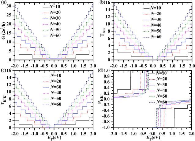
Figure 3.G, T_KK, ${T}_{{K}^{{\prime} }{K}^{{\prime} }}$ and ${P}_{{{KK}}^{{\prime} }}$ versus E_F for ZGNRs with different width N.


In figure 3, we show G, T_KK, ${T}_{{K}^{{\prime} }{K}^{{\prime} }}$ and ${P}_{{{KK}}^{{\prime} }}$ as a function of E_F for pure ZGNRs with different width N. G, T_KK, ${T}_{{K}^{{\prime} }{K}^{{\prime} }}$ and ${P}_{{{KK}}^{{\prime} }}$ show perfect quantized step-like plateaus and the step height of G is 4e²/h. For a pure ZGNR device, the intervalley transmission coefficients (${T}_{{{KK}}^{{\prime} }}$ and ${T}_{{K}^{{\prime} }K}$) are zero. Because the left and right ZGNRs have the same number of conductance channels, which match well at the interface, carriers are not strongly scattered and can transmit only within the same valley. Thus the valley degree of freedom for carriers can be well preserved when they transmit through a pure ZGNR. Step positions of G, T_KK, ${T}_{{K}^{{\prime} }{K}^{{\prime} }}$ and ${P}_{{{KK}}^{{\prime} }}$ are decided by the ribbon width N. As N increases, the energy space between subbands decreases rapidly, so G, T_KK, ${T}_{{K}^{{\prime} }{K}^{{\prime} }}$ and their step numbers increase accordingly. In the bulk gap region of a pure ZGNR, because ${T}_{{K}^{{\prime} }{K}^{{\prime} }}=1$ for E_F > 0 and T_KK = 1 for E_F < 0, the full valley polarization (${P}_{{{KK}}^{{\prime} }}$ = ±1) can be produced by the zigzag edge states. As N increases, the energy region for ${P}_{{{KK}}^{{\prime} }}$ = ±1 decreases, and the step number of ${P}_{{{KK}}^{{\prime} }}$ increases. The plateau height of $| {P}_{{{KK}}^{{\prime} }}| $ are 1, 1/3, 1/5, 1/7, 1/9, etc, as can be derived from equation (3) and can be seen in figures 3(b) and (c), because $| {T}_{{KK}}-{T}_{{K}^{{\prime} }{K}^{{\prime} }}| =1$, and the sum of T_KK and ${T}_{{K}^{{\prime} }{K}^{{\prime} }}$ are 1, 3, 5, 7, 9, etc.

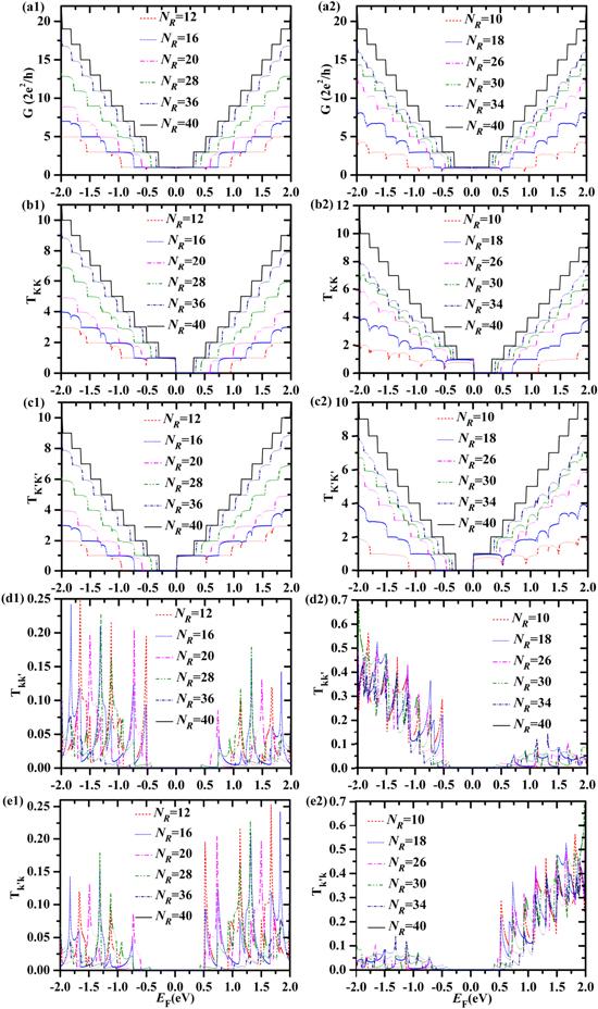
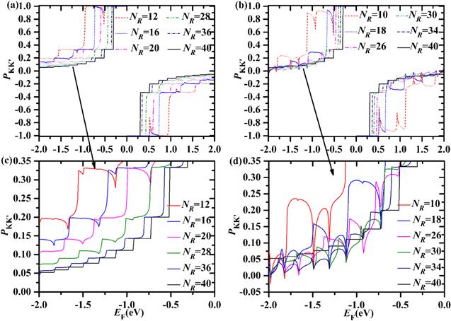
In figures 4 and 5, we show G, T_KK, ${T}_{{{KK}}^{{\prime} }}$, ${T}_{{K}^{{\prime} }K}$, ${T}_{{K}^{{\prime} }{K}^{{\prime} }}$ and ${P}_{{{KK}}^{{\prime} }}$ as a function of E_F for ZGNR junctions with N_L = 40 and different N_R. Compared with pure ZGNRs, the conductance properties of ZGNR junctions show evident differences. Step positions of G, T_KK, ${T}_{{K}^{{\prime} }{K}^{{\prime} }}$ and ${P}_{{{KK}}^{{\prime} }}$ are decided by N_R, their curves still show obvious plateaus when (N_L − N_R)/2 is even, but exhibit sharp dips. Because the left and right ZGNRs have different number of conductance channels, which mismatch at the interface, and carriers are strongly scattered, especially when (N_L − N_R) is large. For (N_L − N_R)/2 being odd, due to the stronger scattering at the mismatched interface, the conductance plateaus are destroyed to a certain degree, G exhibits sharp dips and even oscillation behavior. But in almost the whole bulk gap region of the right ZGNR, ${T}_{{{KK}}^{{\prime} }}=0$, ${P}_{{{KK}}^{{\prime} }}$ = 1, the full valley polarization (${P}_{{{KK}}^{{\prime} }}$ = ±1) can still be remained. This can be ascribed to the zigzag edge states of the right ZGNR. In the bulk gap region of the right ZGNR, carriers transmit completely through the ${K}^{{\prime} }$ valley when E_F > 0 and through the K valley when E_F < 0 [17], assuming the current is right-going in the device. So carriers can transmit only within the same valley, and there are no intervalley transmissions (${T}_{{{KK}}^{{\prime} }}$ and ${T}_{{K}^{{\prime} }K}$ are zero). Therefore, within the gap interval regime, the valley degree of freedom for carriers can be well preserved, implying that the valley polarization efficiency could be high.

Figure 4.

New window|Download| PPT slide
Figure 4.G, T_KK, ${T}_{{K}^{{\prime} }{K}^{{\prime} }}$, ${T}_{{{KK}}^{{\prime} }}$, and ${T}_{{K}^{{\prime} }K}$ versus E_F for ZGNR junctions with N_L = 40 and different N_R. In the left/right panels, (N_L − N_R)/2 is even/odd.


When N_L is fixed and N_R decreases, G, T_KK, ${T}_{{K}^{{\prime} }{K}^{{\prime} }}$ and their step numbers decrease rapidly, they show more and more dips, the energy region for ${P}_{{{KK}}^{{\prime} }}$ = ±1 increases and the step number of ${P}_{{{KK}}^{{\prime} }}$ also decreases, and ${T}_{{{KK}}^{{\prime} }}$ (${T}_{{K}^{{\prime} }K}$) increases outside the bulk gap of the right ZGNR. In figure 5, panels (c) and (d) are the zoom in of panels (a) and (b), respectively, which clearly present the behavior of ${P}_{{{KK}}^{{\prime} }}$ in the high ∣E_F∣ region. As shown in figures 5(a) and (c), when (N_L − N_R)/2 is even, $| {P}_{{{KK}}^{{\prime} }}| $ shows dips outside the bulk gap of the right ZGNR, but the plateaus are basically intact. As shown in figures 5(b) and (d), when (N_L − N_R)/2 is odd, dips of $| {P}_{{{KK}}^{{\prime} }}| $ become deeper, plateaus of ${P}_{{{KK}}^{{\prime} }}$ are broken seriously as N_R decreases to a certain degree. Naturally, the intervalley scattering in a pure ZGNR is vanishing. Nevertheless, in ZGNR junctions, when E_F is not in the bulk gap of the right ZGNR, carriers may be transmitted from one valley to another (${T}_{{{KK}}^{{\prime} }}$ and ${T}_{{K}^{{\prime} }K}$ are not zero), and many deep dips appear in the profile of G, T_KK, ${T}_{{K}^{{\prime} }{K}^{{\prime} }}$ and ${P}_{{{KK}}^{{\prime} }}$, especially when (N_L − N_R)/2 is large and odd, due to the strong scattering of carriers at the mismatched interface. Therefore, in order to strengthen ${T}_{{{KK}}^{{\prime} }}$ (${T}_{{K}^{{\prime} }K}$), we can increase (N_L − N_R)/2 and let it be odd. However, compared with the intravalley transmission coefficients (T_KK and ${T}_{{K}^{{\prime} }{K}^{{\prime} }}$), the intervalley transmission coefficients (${T}_{{{KK}}^{{\prime} }}$ and ${T}_{{K}^{{\prime} }K}$) are much smaller. Thus the intravalley transmission coefficients (T_KK and ${T}_{{K}^{{\prime} }{K}^{{\prime} }}$) contribute dominantly to G. So the valley dependent transport properties of carriers in ZGNR junctions can be manipulated by both N_L and N_R.

Figure 5.

New window|Download| PPT slide
Figure 5.${P}_{{{KK}}^{{\prime} }}$ versus E_F for ZGNR junctions with N_L = 40 and different N_R. In the left (right) panels, (N_L − N_R)/2 is even (odd). The enlarged area in the lower panels clearly present the behavior of ${P}_{{{KK}}^{{\prime} }}$ in the high ∣E_F∣ region.


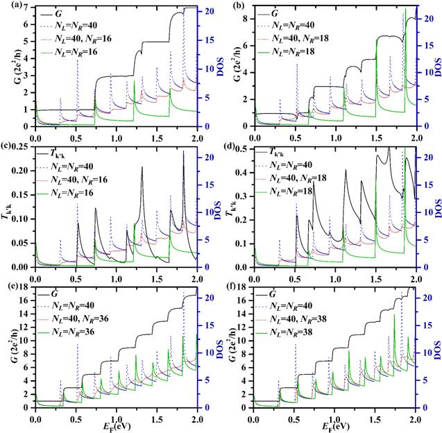
Next, in order to further clarify the complex behavior of G and ${T}_{{K}^{{\prime} }K}$ in ZGNR junctions, we calculate the corresponding density of states (DOS). In figure 6, G, ${T}_{{K}^{{\prime} }K}$ and DOS (the red dot line) versus E_F for ZGNR junctions with N_L = 40 and N_R = 16, 18 , 36 and 38 are shown, the DOS versus E_F for ZGNRs with N_L = N_R = 40, 16, 18, 36 and 38 are also shown for comparison. Obviously, for ZGNR junctions, step and dip positions of G correspond exactly to the peaks of the DOS. For ZGNRs, the DOS (the blue dash line for N = 40 and the green real line for other N) peaks coincide with the edges of the subbands. Either at the subband edges of the left wider or the right narrower ZGNR, the DOS of the ZGNR junction (the red dot line) increases, and even shows peaks. G shows dips at some of the subband edges of the left wider ZGNR where there exists a DOS peak, while G exhibits steps at every subband edge of the right narrower ZGNR, and ${T}_{{K}^{{\prime} }K}$ exhibits peaks at most of the subband edges of both the left and right ZGNRs. Therefore, in ZGNR junctions, dip positions of G are determined by the width of the left wider ZGNR N_L, step positions of G are determined by the width of the right narrower ZGNR N_R, and peak positions of ${T}_{{K}^{{\prime} }K}$ are determined by both N_L and N_R. For a fixed N_L and decreasing N_R, by comparing panel (a)/(b) with panel (e)/(f) in figure 6, we can see that a DOS peak (the red dot line) appears at more and more subband edges of the left wider ZGNR, thus G shows more and more dips and the peaks of ${T}_{{K}^{{\prime} }K}$ become more and more high, especially when (N_L − N_R)/2 is odd. As (N_L − N_R) approaches zero, most dips of G and peaks of ${T}_{{K}^{{\prime} }K}$ disappear, since most of the DOS peaks (the red dot line) located at the subband edges of the left wider ZGNR disappear, especially when ∣E_F∣ is not very large, as shown in figures 6(e) and (f) for N_R = 36 and 38, respectively. Because the energy mismatch between subbands in the left and right ZGNRs decreases, the scattering of carriers at the mismatched interface becomes weaker. The curves of T_KK, ${T}_{{K}^{{\prime} }{K}^{{\prime} }}$, ${T}_{{{KK}}^{{\prime} }}$ and ${P}_{{{KK}}^{{\prime} }}$ versus E_F can be analyzed similarly.

Figure 6.

New window|Download| PPT slide
Figure 6.G, ${T}_{{K}^{{\prime} }K}$ and DOS (the red dot line) versus E_F for ZGNR junctions with N_L = 40 and N_R = 16, 18, 36 and 38, the DOS versus E_F for ZGNRs with N_L = N_R = 40, 16, 18, 36 and 38 are also shown for comparison.

4. Conclusion

In summary, the valley dependent transport properties of ZGNR junctions are studied by the transfer matrix and Green's function method. In the bulk gap region of the right ZGNR, ${T}_{{{KK}}^{{\prime} }}={T}_{{K}^{{\prime} }K}=0$ and the valley polarization ${P}_{{{KK}}^{{\prime} }}$ = ±1, thus the valley polarization can be well preserved. Out of the bulk gap of the right ZGNR, the plateau values of $| {P}_{{{KK}}^{{\prime} }}| $ are 1/3, 1/5, 1/7, 1/9, etc. It is found that step/dip positions of G, T_KK, ${T}_{{K}^{{\prime} }{K}^{{\prime} }}$ and ${P}_{{{KK}}^{{\prime} }}$ can be modulated by N_R/N_L and peaks positions of ${T}_{{{KK}}^{{\prime} }}$ and ${T}_{{K}^{{\prime} }K}$ can be manipulated by both N_L and N_R. As N_R increases, G, T_KK , ${T}_{{K}^{{\prime} }{K}^{{\prime} }}$ and their step numbers increase, the energy region for ${P}_{{{KK}}^{{\prime} }}$ = ±1 decreases. When N_L is fixed and N_R decreases, outside the bulk gap of the right ZGNR, G (T_KK, ${T}_{{K}^{{\prime} }{K}^{{\prime} }}$ and ${P}_{{{KK}}^{{\prime} }}$) shows more and more dips, and ${T}_{{{KK}}^{{\prime} }}$ (${T}_{{K}^{{\prime} }K}$) has more and more high peaks, especially when (N_L − N_R)/2 is odd. So ${T}_{{{KK}}^{{\prime} }}$ and ${T}_{{K}^{{\prime} }K}$ can be strengthened by increasing (N_L − N_R)/2 and letting it be odd. However, compared with the intravalley transmission coefficients (T_KK and ${T}_{{K}^{{\prime} }{K}^{{\prime} }}$), the intervalley transmission coefficients (${T}_{{{KK}}^{{\prime} }}$ and ${T}_{{K}^{{\prime} }K}$) are much smaller. So the intravalley transmission contributes dominantly to G. Our findings may provide valuable guidance for the design and fabrication of valleytronic devices based on ZGNR junctions.

Appendix

Let us introduce the transfer matrix and Green's function method in detail. Assuming the lead is characterized by the unit cell Hamiltonian h and nearest-neighbor hopping matrix t = H_i,i+1. Here the number of basis states in each unit cell is assumed to be M and thus h and t are M × M matrices. The wave propagation in this lead is governed by the uniform Schrödinger equation [9, 41, 42](A1)$\begin{eqnarray}-{t}^{\dagger }{c}_{i-1}+({EI}-h){c}_{i}-{{tc}}_{i+1}=0,\end{eqnarray}$here I is the M × M identity matrix and c_i is a vector of dimension M containing the wave-function coefficients on all sites and/or orbitals of the ith unit cell. Assuming the thickness of each unit cell in the lead is a, and imposing the Bloch symmetry c_i = λc_i−1, c_i+1 = λ²c_i−1 (λ ≡ e^ika is the Bloch factor), the above equation can be written as [9, 41, 42](A2)$\begin{eqnarray}[-{t}^{\dagger }+({EI}-h)\lambda -{\lambda }^{2}t]{c}_{i-1}=0.\end{eqnarray}$

The above equation can be rewritten as a generalized 2M × 2M eigenvalue problem [9, 41](A3)$\begin{eqnarray}\begin{array}{l}\left[\begin{array}{cc}0 & 1\\ -{t}^{\dagger } & {EI}-h\end{array}\right]\left[\begin{array}{c}{c}_{i-1}\\ \lambda {c}_{i-1}\end{array}\right]\\ =\lambda \left[\begin{array}{cc}1 & 0\\ 0 & t\end{array}\right]\left[\begin{array}{c}{c}_{i-1}\\ \lambda {c}_{i-1}\end{array}\right].\end{array}\end{eqnarray}$

For a given energy E and without imposing any boundary conditions, equation (A3) can be solved to yield 2M eigenmodes, which are classified into M right-going ones and M left-going ones according to the characteristics of their corresponding k (λ) [41]. The eigenvalues are denoted as λ_±,i where i = 1, · · · , M, and the corresponding eigenvectors are u_±,i, which are M × 1 matrices. Here + and − correspond to the right-going and left-going waves, respectively.

The propagation matrices P_± for left-going and right-going waves can be written as [9, 40–42](A4)$\begin{eqnarray}{P}_{\pm }={U}_{\pm }\left[\begin{array}{ccc}{\lambda }_{\pm ,1} & & \\ & \ddots & \\ & & {\lambda }_{\pm ,M}\end{array}\right]{U}_{\pm }^{-1},\end{eqnarray}$with ${U}_{\pm }=[\left|{u}_{\pm ,1}\right\rangle ,\cdot \cdot \cdot ,\left|{u}_{\pm ,M}\right\rangle ]$. The group velocity of the eigenmode i in the p lead can be calculated by [41, 42](A5)$\begin{eqnarray}{v}_{\pm ,i}^{p}=-\displaystyle \frac{2a}{{\hslash }}\mathrm{Im}\left\langle {u}_{\pm ,i}\right|{\lambda }_{\pm ,i}t\left|{u}_{\pm ,i}\right\rangle .\end{eqnarray}$

Generally, the layered system can be divided into the semi-infinite left lead L, the central region C (unit cells 1 ≤ m ≤ N), and the semi-infinite right lead R. The Green's function of the central region can be expressed as(A6)$\begin{eqnarray}G={[E+{\rm{i}}{0}^{+}-H-{{\rm{\Sigma }}}^{L}-{{\rm{\Sigma }}}^{R}]}^{-1},\end{eqnarray}$where H is the effective Hamiltonian for the central region, and Σ^L,R are self-energy corrections due to the left and right leads, which can be calculated by [41, 42](A7)$\begin{eqnarray}{{\rm{\Sigma }}}^{L}={t}_{L}^{\dagger }{\left({P}_{-}^{L}\right)}^{-1},{{\rm{\Sigma }}}^{R}={t}_{R}{P}_{+}^{R}.\end{eqnarray}$

The physical transmission matrix element from the right-going eigenmode i in the left terminal to the right-going eigenmode j in the right terminal is computed by [32, 40–44](A8)$\begin{eqnarray}{t}_{{ij}}(E)=\sqrt{\displaystyle \frac{{v}_{+,j}^{R}{a}_{L}}{{v}_{+,i}^{L}{a}_{R}}}{\left({U}_{+,j}^{R}\right)}^{-1}{G}_{N,1}{Q}_{0}{U}_{+,i}^{L},\end{eqnarray}$here ${Q}_{0}=(E+{\rm{i}}{0}^{+})I-h-{t}_{L}^{\dagger }{\left({P}_{-}^{L}\right)}^{-1}-{t}_{R}{P}_{+}^{L}$, G_N,1 is the (N, 1) block of G, which relates the first unit cell to the last unit cell of the central region, and a_L (a_R) is the thickness of the unit cell in the left (right) lead.

Thus the valley-resolved transmission coefficients are obtained by collecting t_ij in two separate valleys (K and ${K}^{{\prime} }$), and the transmission coefficient from valley K in the left terminal to valley ${K}^{{\prime} }$ in the right terminal is [32, 44](A9)$\begin{eqnarray}{T}_{{{KK}}^{{\prime} }}(E)=\sum _{i\in K}\sum _{j\in {K}^{{\prime} }}{\left|{t}_{{ij}}(E)\right|}^{2}.\end{eqnarray}$

Acknowledgments

This work was supported by the Natural Science Foundation of Henan Province under Grant No. 212300410388, and the “316” Project Plan of Xuchang University.

Reference View Option By original order
By published year
By cited within times
By Impact factor

[1]Goerbig M O Fuchs J N Kechedzhi K Falko V I 2007 Phys. Rev. Lett. 99 087402
DOI:10.1103/PhysRevLett.99.087402 [Cited within: 1]

[2]Gusynin V P Sharapov S G Carbotte J P 2007 Phys. Rev. Lett. 98 157402
DOI:10.1103/PhysRevLett.98.157402

[3]Zhang Z Z Chang K Peeters F M 2008 Phys. Rev. B 77 235411
DOI:10.1103/PhysRevB.77.235411 [Cited within: 2]

[4]Bolotin K I Sikes K J Jiang Z Fudenberg G Hone J Kim P Stormer H L 2008 Solid State Commun. 146 351
DOI:10.1016/j.ssc.2008.02.024 [Cited within: 1]

[5]Balandin A A Ghosh S Bao W Calizo I Teweldebrhan D Miao F Lau C N 2008 Nano Lett. 8 902
DOI:10.1021/nl0731872

[6]Novoselov K S Geim A K Morozov S V Jiang D Zhang Y Dubonos S V Grigorieva I V Firsov A A 2004 Science 306 666
DOI:10.1126/science.1102896

[7]Gunlycke D White C T 2011 Phys. Rev. Lett. 106 136806
DOI:10.1103/PhysRevLett.106.136806 [Cited within: 2]

[8]Zhang Z Z Chang K Chan K S 2008 Appl. Phys. Lett. 93 062106
DOI:10.1063/1.2970957 [Cited within: 2]

[9]Zhang Z Z Wu Z H Chang K Peeters F M 2009 Nanotechnology 20 415203
DOI:10.1088/0957-4484/20/41/415203 [Cited within: 4]

[10]Wu Z H Zhang Z Z Chang K Peeters F M 2010 Nanotechnology 21 185201
DOI:10.1088/0957-4484/21/18/185201 [Cited within: 2]

[11]Li H D Wang L Lan Z H Zheng Y S 2009 J. Appl. Phys. 105 013703
DOI:10.1063/1.3054449 [Cited within: 2]

[12]Hong S Yoon Y Guo J 2008 Appl. Phys. Lett. 92 083107
DOI:10.1063/1.2885095 [Cited within: 1]

[13]Li T C Lu S P 2008 Phys. Rev. B 77 085408
DOI:10.1103/PhysRevB.77.085408

[14]Xu Z P Zheng Q S 2007 Appl. Phys. Lett. 90 223115
DOI:10.1063/1.2745268 [Cited within: 1]

[15]Wu Y Childs P A 2011 Nanoscale Res. Lett. 6 62
DOI:10.1007/s11671-010-9791-y [Cited within: 1]

[16]Li M Han H P Feng Z B Zhao Z Y 2019 Physica E 111 172
DOI:10.1016/j.physe.2019.03.020 [Cited within: 1]

[17]Shen M Zhang Y Y An X T Liu J J Li S S 2014 J. Appl. Phys. 115 233702
DOI:10.1063/1.4883193 [Cited within: 3]

[18]Castro Neto A H Guinea F Peres N M R Novoselov K S Geim A K 2009 Rev. Mod. Phys. 81 109
DOI:10.1103/RevModPhys.81.109

[19]Wu Q P Chang L L Li Y Z Liu Z F Xiao X B 2020 Nanoscale Res. Lett. 15 46
DOI:10.1186/s11671-020-3275-5 [Cited within: 1]

[20]Xiao D Yao W Niu Q 2007 Phys. Rev. Lett. 99 236809
DOI:10.1103/PhysRevLett.99.236809 [Cited within: 2]

[21]Rycerz A Tworzydlo J Beenakker C W J 2007 Nat. Phys. 3 172
DOI:10.1038/nphys547 [Cited within: 2]

[22]Pereira J MJrPeeters F M Filho R N C Farias G A 2009 J. Phys.: Condens. Matter 21 045301
DOI:10.1088/0953-8984/21/4/045301

[23]Zhai F Zhao X F Chang K Xu H Q 2010 Phys. Rev. B 82 115442
DOI:10.1103/PhysRevB.82.115442

[24]Jiang Y J Low T Chang K Katsnelson M I Guinea F 2013 Phys. Rev. Lett. 110 046601
DOI:10.1103/PhysRevLett.110.046601

[25]Wu Z H Zhai F Peeters F M Xu H Q Chang K 2011 Phys. Rev. Lett. 106 176802
DOI:10.1103/PhysRevLett.106.176802 [Cited within: 3]

[26]Aufray B Kara A Vizzini S Oughaddou H Leandri C Ealet B Le Lay G 2010 Appl. Phys. Lett. 96 183102
DOI:10.1063/1.3419932 [Cited within: 1]

[27]Mak K F Lee C Hone J Shan J Heinz T F 2010 Phys. Rev. Lett. 105 136805
DOI:10.1103/PhysRevLett.105.136805 [Cited within: 1]

[28]Zeng H Dai J Yao W Xiao D Cui X 2012 Nat. Nanotechnol. 7 490
DOI:10.1038/nnano.2012.95 [Cited within: 1]

[29]Mak K F McGill K L Park J McEuen P L 2014 Science 344 1489
DOI:10.1126/science.1250140

[30]Shimazaki Y Yamamoto M Borzenets I V Watanabe K Taniguchi T Tarucha S 2015 Nat. Phys. 11 1032
DOI:10.1038/nphys3551

[31]Pan H Li X Zhang F Yang S Y A 2015 Phys. Rev. B 92 041404(R)
DOI:10.1103/PhysRevB.92.041404 [Cited within: 1]

[32]Cheng S G Zhou J J Jiang H Sun Q F 2016 New J. Phys. 18 103024
DOI:10.1088/1367-2630/18/10/103024 [Cited within: 6]

[33]Zhang L Gong K Chen J Z Liu L Zhu Y Xiao D Guo H 2014 Phys. Rev. B 90 195428
DOI:10.1103/PhysRevB.90.195428 [Cited within: 1]

[34]Haldane F D M 1988 Phys. Rev. Lett. 61 2015
DOI:10.1103/PhysRevLett.61.2015 [Cited within: 1]

[35]Long W Sun Q F Wang J 2008 Phys. Rev. Lett. 101 166806
DOI:10.1103/PhysRevLett.101.166806

[36]Li J Shen S Q 2008 Phys. Rev. B 78 205308
DOI:10.1103/PhysRevB.78.205308

[37]Beenakker C W J 2008 Rev. Mod. Phys. 80 1337
DOI:10.1103/RevModPhys.80.1337 [Cited within: 1]

[38]Ezawa M 2006 Phys. Rev. B 73 045432
DOI:10.1103/PhysRevB.73.045432 [Cited within: 1]

[39]Wakabayashi K Fujita M Ajiki H Sigrist M 1999 Phys. Rev. B 59 8271
DOI:10.1103/PhysRevB.59.8271 [Cited within: 1]

[40]Ando T 1991 Phys. Rev. B 44 8017
DOI:10.1103/PhysRevB.44.8017 [Cited within: 3]

[41]Zhang S H Yang W Chang K 2017 Phys. Rev. B 95 075421
DOI:10.1103/PhysRevB.95.075421 [Cited within: 6]

[42]Khomyakov P A Brocks G Karpan V Zwierzycki M Kelly P J 2005 Phys. Rev. B 72 035450
DOI:10.1103/PhysRevB.72.035450 [Cited within: 5]

[43]Cheng S G Liu H W Jiang H Sun Q F Xie X C 2018 Phys. Rev. Lett. 121 156801
DOI:10.1103/PhysRevLett.121.156801

[44]Cheng S G Zhang R Z Zhou J J Jiang H Sun Q F 2018 Phys. Rev. B 97 085420
DOI:10.1103/PhysRevB.97.085420 [Cited within: 4]

[45]Fisher D S Lee P A 1981 Phys. Rev. B 23 6851
DOI:10.1103/PhysRevB.23.6851 [Cited within: 1]