Yu-Jiao Bo^,, Wen-Wen Li^,, Yu-Chen Guo^,, Ji-Chong Yang^,∗Department of Physics, Liaoning Normal University, Dalian 116029, China

First author contact: ∗Author to whom any correspondence should be addressed.
Received:2021-04-11Revised:2021-04-30Accepted:2021-05-1Online:2021-06-01


Abstract
Compared with the traditional magnetic bubble, a skyrmion has a smaller size, and better stability and therefore is considered as a very promising candidate for future memory devices. When skyrmions are manipulated, erased and created, the density of skyrmions can be varied, however the relationship between the radii and the densities of skyrmions needs more exploration. In this paper, we study this problem both theoretically and by using the lattice simulation. The average radius of skyrmions as a function of material parameters, the strength of the external magnetic field and the density of skyrmions is obtained and verified. With this explicit function, the skyrmion radius can be easily predicted, which is helpful for the future study of skyrmion memory devices.
Keywords： radius of a skyrmion;shape of a skyrmion;lattice simulation


PDF (2357KB)MetadataMetricsRelated articlesExportEndNote|Ris|BibtexFavorite
Cite this article
Yu-Jiao Bo, Wen-Wen Li, Yu-Chen Guo, Ji-Chong Yang. The relation between the radii and the densities of magnetic skyrmions. Communications in Theoretical Physics, 2021, 73(7): 075701- doi:10.1088/1572-9494/abfda0

1. Introduction

Skyrmion is a topological soliton originally proposed to describe the baryons [1]. In condensed matter, a particle-like object known as magnetic skyrmion was introduced theoretically in 1989 [2]. It was observed for the first time in 2D magnetic systems [3–6] involving Dzyaloshinskii-Moriya interactions (DMI) [7, 8]. Compared with the traditional magnetic bubble, the skyrmion is smaller, more stable and needs lower power to manipulate, therefore, it has been proposed that the skyrmion is a promising candidate for high density, high stability, high speed, high storage and low energy consumption memory devices [9–11]. As a result, the magnetic skyrmions have drawn a lot of attention and been studied intensively recently [11–15].

A prerequisite for the use of skyrmions in devices is the knowledge of the relationship between the size of a skyrmion and parameters such as exchange strength, DMI strength and the strength of external magnetic field. Such a relationship can be investigated by solving the Euler–Lagrange equation of a skyrmion, for example numerically [16] or by using an ansatz [9], or by using the harmonic oscillation expansion [17], or by an asymptotic matching [18]. It has been noticed that the radius of a skyrmion in the skyrmion phase is much smaller than that of an isolated skyrmion [17]. Both the radii of an isolated skyrmion and the skyrmions in the skyrmion lattice were studied quantitatively in [19]. In particular, numerical results were obtained for the equilibrium radii of skyrmion lattices.

However, as a potential candidate for storage, the skyrmion is meant to be manipulated, erased and created. In this case, the number of skyrmions can vary from only just one to filling the entire skyrmion lattice. The transformation of a skyrmion lattice to the saturated state is continuous, in this process, the skyrmion lattice gradually decomposes into isolated skyrmions in the saturated state [15]. In this paper, we study the average radius of skyrmions with the density of skyrmions in the range between a single isolated skyrmion and the skyrmion lattice. While the results have been obtained for a single isolated skyrmion, and for skyrmion lattices, up to our knowledge, the radius of a skyrmion when the density of the skyrmions is between the skyrmion lattice and the single isolated skyrmion is poorly understood at a quantitative level.

The rest of the paper is organized as the following. The analytical and numerical results based on circular cell approximation are established in section 2. In section 3, we introduce the lattice simulation of Landau–Lifshitz-Gilbert (LLG) equation. We compare the theoretical results with the results of lattice simulation in section 4. A summary is made in section 5.

2. Circular cell approximation

The local magnetic moment of a skyrmion can be parameterized as(1)$\begin{eqnarray}{\boldsymbol{n}}(r,\phi ,z)=\sin [m\theta (r)+\gamma ]{{\boldsymbol{e}}}_{\phi }+g\cos [\theta (r)]{{\boldsymbol{e}}}_{z},\end{eqnarray}$where r, φ, z are coordinates in a cylindrical coordinate, γ is the helicity angle, m = 1 for a skyrmion and m = −1 for an anti-skyrmion, g = ± 1. The skyrmion number is Q = − mg. In the following, we only consider the skyrmion with Q = 1 (m = 1, g = − 1).

By using the circular cell approximation, the skyrmions are viewed as sitting in circular cells with radius R, which means the boundary condition θ(0) = π and θ(R) = 0 [19]. In principle, θ(r) can be expanded using any Hilbert space. Since the wave-function of the ground state of the harmonic oscillator and the numerical solution of the Euler–Lagrange equation of a skyrmion are close in shape [17], we use the Hilbert space of harmonic oscillator to expand θ(r). We do not require $\theta ^{\prime} (r)=0$ as in [17] because $\theta ^{\prime} (r)\ne 0$ is allowed by the Euler–Lagrange equation, therefore the eigen-functions of odd energy levels are also included. To impose the boundary conditions θ(0) = π and θ(R) = 0, θ(r) to the next-to-next-to leading order can be written as(2)$\begin{eqnarray}\begin{array}{l}\theta (r)=\displaystyle \sum _{n=0}^{2}{C}_{n}{\phi }_{n}(r)=\pi {{\rm{e}}}^{-\tfrac{\omega {r}^{2}}{2}}\\ \quad -\displaystyle \frac{1+{{cR}}^{2}}{R}r\pi {{\rm{e}}}^{-\tfrac{\omega {r}^{2}}{2}}+c\pi {r}^{2}{{\rm{e}}}^{-\tfrac{\omega {r}^{2}}{2}},\end{array}\end{eqnarray}$where φ_n are eigen-functions of harmonic oscillator, ω and c are parameters to be determined. By assuming the coefficients of the higher order terms are small, the power counting yields c ∼ 1/R² and 1/R ≪ 1.

We concentrate on the case when the anisotropy is absent, the energy to be minimized is $F=2\pi {\int }_{0}^{R}{\rm{d}}{rr}{ \mathcal F }(r)$ with the energy density(3)$\begin{eqnarray}\begin{array}{l}{ \mathcal F }(r)=2J\left\{\left[{\left(\displaystyle \frac{1}{2}\displaystyle \frac{\partial \theta }{\partial r}+\displaystyle \frac{d}{2}\right)}^{2}-{\left(\displaystyle \frac{d}{2}\right)}^{2}\right.\right.\\ \quad \left.\left.+\displaystyle \frac{{\sin }^{2}(\theta )}{4{r}^{2}}+\displaystyle \frac{d\sin (2\theta )}{4r}\right]-\displaystyle \frac{b}{2}(\cos (\theta )-1)\right\},\end{array}\end{eqnarray}$where d ≡ D/J and b ≡ B/J, J is the strength of local ferromagnetic exchange, D is the strength of DMI, B is the strength of the external magnetic field which is assumed to be parallel to the z-axis. For simplicity, we consider dimensionless parameters, the matching is discussed in section 4.4.

Denoting s ≡ 1/R, F can be expanded as $F=\hat{F}+{ \mathcal O }({s}^{5})$ with(4)$\begin{eqnarray}\begin{array}{rcl}\hat{F} & = & -\frac{1}{72{s}^{4}{\omega }^{3}}\left\{-36{\pi }^{3}{{bc}}^{2}{s}^{4}{f}_{\mathrm{1,2},\mathrm{1,0}}+12{\pi }^{3}{bs}\sqrt{\omega }\left(c+{s}^{2}\right)\right.\\ & & \times \ \left(6{{cs}}^{2}{f}_{1,\tfrac{3}{2},\mathrm{1,0}}-\pi {f}_{\tfrac{3}{2},\tfrac{3}{2},\mathrm{0,1}}{\left(c+{s}^{2}\right)}^{2}\right)\\ & & +3{\pi }^{5}{{bf}}_{\mathrm{2,2},\mathrm{1,0}}{\left(c+{s}^{2}\right)}^{4}+36{\pi }^{4}{{bcs}}^{2}{f}_{\tfrac{3}{2},\mathrm{2,0,1}}{\left(c+{s}^{2}\right)}^{2}\\ & & +72{\pi }^{2}{{bs}}^{3}{\omega }^{3/2}{f}_{\tfrac{1}{2},\tfrac{1}{2},\mathrm{0,1}}\left(c+{s}^{2}\right)\\ & & +144{\pi }^{3}{c}^{2}d{s}^{4}\sqrt{\omega }{f}_{1,\tfrac{3}{2},\mathrm{1,1}}-144{\pi }^{2}{{cds}}^{4}{\omega }^{3/2}{f}_{\tfrac{1}{2},\tfrac{1}{2},\mathrm{2,0}}\\ & & +144{\pi }^{3}d{s}^{2}{\omega }^{3/2}{f}_{1,\tfrac{1}{2},\mathrm{1,1}}{\left(c+{s}^{2}\right)}^{2}\\ & & -48{\pi }^{5}d\sqrt{\omega }{f}_{2,\tfrac{3}{2},\mathrm{1,1}}{\left(c+{s}^{2}\right)}^{4}\\ & & +288{\pi }^{4}{{cds}}^{2}\sqrt{\omega }{f}_{\tfrac{3}{2},\tfrac{3}{2},\mathrm{2,0}}{\left(c+{s}^{2}\right)}^{2}\\ & & -24{\pi }^{3}s{\omega }^{3/2}\left(c+{s}^{2}\right)\left(3{{cs}}^{2}\left({f}_{1,\tfrac{1}{2},\mathrm{0,2}}-{f}_{1,\tfrac{1}{2},\mathrm{2,0}}\right)\right.\\ & & \left.+2\pi {f}_{\tfrac{3}{2},\tfrac{1}{2},\mathrm{1,1}}{\left(c+{s}^{2}\right)}^{2}\right)\\ & & +72{\pi }^{2}{s}^{3}{\omega }^{5/2}{f}_{\tfrac{1}{2},-\tfrac{1}{2},\mathrm{1,1}}\left(c+{s}^{2}\right)-72\pi d{s}^{4}{\omega }^{5/2}{f}_{0,-\tfrac{1}{2},\mathrm{1,1}}\\ & & -36\pi {s}^{4}{\omega }^{3}{f}_{0,-\mathrm{1,0,2}}\\ & & +36{s}^{2}\omega \left[4\pi b\left({c}^{2}(-\mathrm{Ci}(\pi )+{\gamma }_{E}-2+\mathrm{log}(\pi ))-4{{cs}}^{2}\right.\right.\\ & & \left.+{s}^{4}(-\mathrm{Ci}(\pi )+{\gamma }_{E}-2+\mathrm{log}(\pi )\right)\\ & & \left.+4{\pi }^{5/2}\sqrt{2}{{cds}}^{2}\sqrt{\omega }-{\pi }^{3}\omega {\left(c+{s}^{2}\right)}^{2}\right]\\ & & -144\pi {{bs}}^{4}{\omega }^{2}(-\mathrm{Ci}(\pi )+{\gamma }_{E}+\mathrm{log}(\pi ))\\ & & +18\pi \omega \left({c}^{4}+{s}^{8}\right)(-\mathrm{Ci}(2\pi )+{\gamma }_{E}+\mathrm{log}(2\pi ))\\ & & +3\pi s\omega \left[16d\mathrm{Si}(2\pi )\left({c}^{3}+{s}^{6}\right)+16\pi d{\left(c+{s}^{2}\right)}^{3}\right.\\ & & \left.+15{\pi }^{5/2}{{cs}}^{2}\sqrt{\omega }\left(c+{s}^{2}\right)\right]-12{\pi }^{3}\omega \\ & & \left({c}^{4}+4{c}^{3}{s}^{2}+12{c}^{2}{s}^{4}+4{{cs}}^{6}+{s}^{8}\right)\\ & & -16{\pi }^{9/2}\sqrt{6}{{cds}}^{2}\sqrt{\omega }{\left(c+{s}^{2}\right)}^{2}+18{\pi }^{2}{s}^{3}{\omega }^{2}\\ & & \times \ \left(c+{s}^{2}\right)\left({\pi }^{3/2}\sqrt{\omega }-8d\right)\\ & & \left.+72{\pi }^{5/2}\sqrt{2}d{s}^{4}{\omega }^{5/2}-36{\pi }^{3}{s}^{4}{\omega }^{3}\right\},\end{array}\end{eqnarray}$where γ_E is the Euler constant, Ci and Si are cosine and sine integral functions, and ${f}_{m,n,{n}_{c},{n}_{s}}$ are constant numbers defined as(5)$\begin{eqnarray}{f}_{m,n,{n}_{c},{n}_{s}}\equiv {\int }_{0}^{\infty }{\rm{d}}x{{\rm{e}}}^{-{mx}}{x}^{n}{\cos }^{{n}_{c}}\left(\pi {{\rm{e}}}^{-\tfrac{{x}^{2}}{2}}\right){\sin }^{{n}_{s}}\left(\pi {{\rm{e}}}^{-\tfrac{{x}^{2}}{2}}\right).\end{eqnarray}$This seemingly lengthy expression of $\hat{F}$ is nothing more than a polynomial of $\sqrt{\omega }$ and c. To achieve a higher precision, in principle, both the expansions of θ(r) and F can be worked out for higher orders.

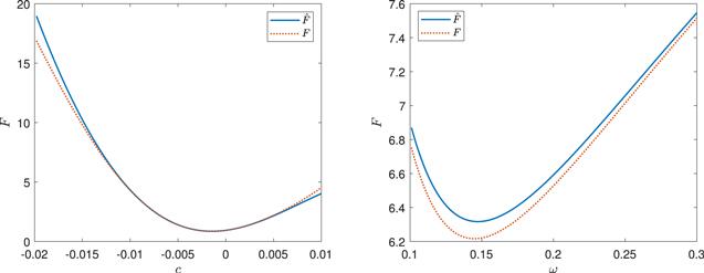
For d = 0.4, b = 0.1, R = 20, in the region that ω ∼ 0.15 and c ∼ − 0.01, we compare F with $\hat{F}$ in figure 1. $\hat{F}$ can approximate F well in the region concerned. Especially, the positions where F and $\hat{F}$ are minimized fit each other very well. To minimize F, we use variational method, so that there are two equations ∂F/∂ω = 0 and ∂F/∂c = 0, by which ω and c can be solved.

Figure 1.

New window|Download| PPT slide
Figure 1.Compare F with $\hat{F}$ at d = 0.4, b = 0.1, R = 20. The left panel is F and $\hat{F}$ at ω = 0.15 as functions of c, the right panel is F and $\hat{F}$ at c = − 0.012 as functions of ω.


By setting a threshold h such that the sites with n_z < h are determined as inside a skyrmion, the radius of a skyrmion can be obtained by solving the equation $\cos (\theta (r))=h$. Considering the leading order approximation which corresponds to c = s = 0 (denoted as θ_LO), by solving $\cos ({\theta }_{\mathrm{LO}}(r))=h$, the radius of a skyrmion (denoted as r_s) is approximately(6)$\begin{eqnarray}{r}_{s}=\sqrt{\displaystyle \frac{2}{\omega }\mathrm{log}\left(\displaystyle \frac{\pi }{{\cos }^{-1}(h)}\right)},\end{eqnarray}$where ω can be solved by the equations $\partial \hat{F}/\partial \omega \,=\partial \hat{F}/\partial c=0$ mentioned above. We choose the solution that ω and c are real numbers, and ∣c∣ ≪ 1.

With the numerical solutions of ω, we can investigate the change of r_s as function of s. For this purpose, we define $\hat{r}={r}_{s}/{r}_{\mathrm{iso}}$ where r_s is calculated by ω solved at s, and r_iso is the radius of a single isolated skyrmion which is calculated by ω solved at s → 0.

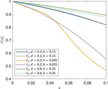
Since the numerical solutions are inconvenient to use, we fit the solutions as bilinear function of s around d ∼ 0.4, with the numerical solution of $\hat{r}$ denoted as ${\hat{r}}_{n}$ and the fitted solution denoted as ${\hat{r}}_{f}$, the result is ${\hat{r}}_{n}\approx {\hat{r}}_{f}$ with(7)$\begin{eqnarray}\begin{array}{l}{\hat{r}}_{f}\approx 1+\left(105.837{b}^{2}-197.435{bd}+55.6138b\right.\\ \left.+62.0744{d}^{2}-22.544d-0.873711\right)s\\ +\left(-653.657{b}^{2}+1108.47{bd}-301.911b\right.\\ \left.-483.322{d}^{2}+310.55d-60.965\right){s}^{2}\end{array}\end{eqnarray}$${\hat{r}}_{f}$ is compared with ${\hat{r}}_{n}$ in figure 2. It can be found that, for most cases $\hat{r}$ is smaller than 1 and is decreasing with the growth of s, which indicates that the skyrmions become smaller with the growth of density even when b and d are unchanged.

Figure 2.

New window|Download| PPT slide
Figure 2.${\hat{r}}_{f}$ Compared with ${\hat{r}}_{n}$.


We define the density of skyrmions as ρ = N/A where N is the number of skyrmions within an area A. R is approximately half of the average distance between the skyrmions, therefore R can be related to ρ. Assuming the skyrmions are distributed homogenously, then N ≈ A/πR², and $s\approx \sqrt{\pi N/A}$.

It has been found that, by using the leading order ansatz θ_LO, to minimize F yields ω = w₀b²/d² where w₀ = 0.768548 is a constant [17]. By using equation (6), the average radius r_s can be written as(8)$\begin{eqnarray}{r}_{s}(b,d,N)=\sqrt{\displaystyle \frac{2}{{w}_{0}}\mathrm{log}\left(\displaystyle \frac{\pi }{{\cos }^{-1}(h)}\right)}\times \displaystyle \frac{d}{b}\times \hat{r}\left(s=\sqrt{\displaystyle \frac{\pi N}{A}}\right).\end{eqnarray}$

For a skyrmion, n_z varies from −1 to 1 from the center to the edge, and the radius is determined by the number of sites with n_z < 1. But n_z only approaches 1, so we need to set a threshold slightly smaller than 1. If the approximate expression for θ(r) is sufficiently precise, the radius of the skyrmion is consistent as long as we choose a same h for theoretical predictions, lattice simulations and experimental measurements, and the verification of the theory is independent of the specific value of h taken. In this paper we choose 0.9 which is close to 1, other choices would lead to small differences, but would not change the conclusion. Then $\sqrt{2\mathrm{log}\left(\pi /{\cos }^{-1}(h)\right)/{w}_{0}}\approx 2.247\,44$, using ${\hat{r}}_{f}$ to approximate $\hat{r}$,(9)$\begin{eqnarray}\begin{array}{l}{r}_{s}(b,d,\rho )\approx \displaystyle \frac{2.247d}{b}\left\{1+\left[d(975.6-1518.4d)\right.\right.\\ \left.-2053.5{b}^{2}+b(3482.4d-948.481)-191.5\right]\rho \\ +\left[b(98.57-349.9d)+187.6{b}^{2}\right.\\ \left.\left.+d(110.0d-39.96)-1.549\right]\sqrt{\rho }\right\}.\end{array}\end{eqnarray}$

In [19], the equilibrium R is numerically solved by minimize the energy density. Note that R in this case is independent of the density of the skyrmions. In our case, R is a quantity between the case of skyrmion lattice and the case of a single isolated skyrmion, and is determined by the density of the skyrmions, one can calculate r_s after R is given.

3. Lattice simulation

The lattice simulation is based on the LLG equation, denoting n_r as the local magnetic momentum at site r, the LLG can be written as [20–23](10)$\begin{eqnarray}\displaystyle \frac{{\rm{d}}}{{\rm{d}}t}{{\boldsymbol{n}}}_{{\boldsymbol{r}}}=-{{\boldsymbol{B}}}_{\mathrm{eff}}({\boldsymbol{r}})\times {{\boldsymbol{n}}}_{{\boldsymbol{r}}}-\alpha {{\boldsymbol{n}}}_{{\boldsymbol{r}}}\times \displaystyle \frac{{\rm{d}}}{{\rm{d}}t}{{\boldsymbol{n}}}_{{\boldsymbol{r}}},\end{eqnarray}$where n_r is the local magnetic moment, α is the Gilbert damping constant and the effective magnetic field B_eff is(11)$\begin{eqnarray}{{\boldsymbol{B}}}_{\mathrm{eff}}({\boldsymbol{r}})=-\displaystyle \frac{\delta H}{\delta {{\boldsymbol{n}}}_{{\boldsymbol{r}}}},\end{eqnarray}$with the discretized version of Hamiltonian defined as [24, 25](12)$\begin{eqnarray}H=\sum _{{\boldsymbol{r}},i=x,y}\left[-J({\boldsymbol{r}}){{\boldsymbol{n}}}_{{\boldsymbol{r}}+{\delta }_{i}}-D({\boldsymbol{r}}){{\boldsymbol{n}}}_{{\boldsymbol{r}}+{\delta }_{i}}\times {{\boldsymbol{e}}}_{i}-{\boldsymbol{B}}\right]\cdot {{\boldsymbol{n}}}_{{\boldsymbol{r}}},\end{eqnarray}$where δ_i refers to each neighbor. On a square lattice, one has δ_i = e_i, therefore(13)$\begin{eqnarray}\begin{array}{l}{{\boldsymbol{B}}}_{\mathrm{eff}}({\boldsymbol{r}})=\displaystyle \sum _{i=x,y}\left[J({\boldsymbol{r}}){{\boldsymbol{n}}}_{{\boldsymbol{r}}+{\delta }_{i}}+J({\boldsymbol{r}}-{\delta }_{i}){{\boldsymbol{n}}}_{{\boldsymbol{r}}-{\delta }_{i}}\right]\\ +\displaystyle \sum _{i=x,y}\left[D({\boldsymbol{r}}){{\boldsymbol{n}}}_{{\boldsymbol{r}}+{\delta }_{i}}\times {{\boldsymbol{e}}}_{i}-D({\boldsymbol{r}}-{\delta }_{i}){{\boldsymbol{n}}}_{{\boldsymbol{r}}-{\delta }_{i}}\times {{\boldsymbol{e}}}_{i}\right]+{\boldsymbol{B}}({\boldsymbol{r}}).\end{array}\end{eqnarray}$The simulation was carried out on the GPU [20] which has a great advantage over CPUs because of the ability of parallel computing of the GPU. Equation (1) is numerically integrated by using the fourth-order Runge-Kutta method.

4. Numerical results

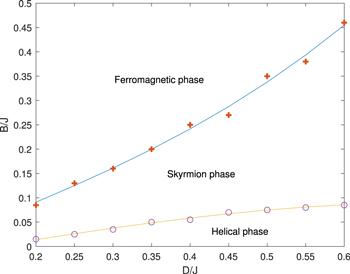
We run the simulation on a 512 × 512 square lattice. In the simulation, we use dimensionless homogeneous J, D and B. J = 1 is used as the definition of the energy unit [25–27], the results are presented with d and b. In the previous works, the Gilbert constant was chose to be α = 0.01 to 1 [21, 23, 26–35]. In this work, we use α = 0.04 which is in the region of commonly used α. The time step is denoted as Δt. We use Δt = 0.01 time unit, and the configurations typically become stable after about 10⁶−10⁷ steps starting with a randomized initial state. The average radius of the skyrmions is measured as r_s = A_s/NA where A_s is the total area of the skyrmions which is determined by the number of sites in the isoheight n_z = h with h = 0.9, A = 512² and N is the number of skyrmions. The standard errors of the radii of skyrmions are also measured.

To investigate the relationship between r, d and b, we simulate with d in the range of 0.2−0.6, and with growing b for each fixed d. We focus on those configurations that are in the skyrmion phase when stable. The phase diagram is shown in figure 3.

Figure 3.

New window|Download| PPT slide
Figure 3.The phase diagram obtained by lattice simulation of LLG with randomized initial states.

4.1. The relationship between the average radius and density

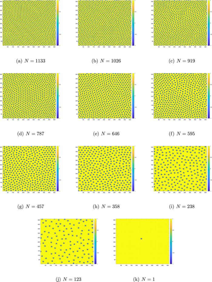
In this subsection, we use the configurations at d = 0.2, b = 0.025, d = 0.35, b = 0.1, d = 0.4, b = 0.1, d = 0.4, b = 0.2, d = 0.45, b = 0.15 and d = 0.6, b = 0.15 to investigate the relationship between the average radius and density. Firstly we calculate the number of skyrmions in each configuration. By repeatedly and randomly erasing about 10% of the total number of skyrmions at a time and performing the simulation sequentially, we obtain the configurations at different N. Taking the case of d = 0.4, b = 0.1 as an example, the resulting configurations are shown in figure 4.

Figure 4.

New window|Download| PPT slide
Figure 4.The configurations corresponding to different N.


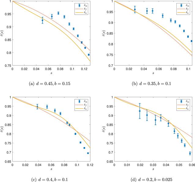
Because the size of the lattice is 512 × 512, $s\approx \sqrt{N\pi /{512}^{2}}\approx 0.003\,46\sqrt{N}$. The ratios of the average radii of skyrmions at different N to the radius of an isolated skyrmion are measured and denoted as ${\hat{r}}_{m}$. We compare ${\hat{r}}_{m}$, ${\hat{r}}_{f}$ and ${\hat{r}}_{n}$ in figure 5. It can be seen that the theocratical results ${\hat{r}}_{n}$ and ${\hat{r}}_{f}$ can approximately predict ${\hat{r}}_{m}$ correctly, the deviations between ${\hat{r}}_{m}$ and ${\hat{r}}_{s,f}$ are generally within about 10%. Besides, for larger skyrmions, the theocratical results are generally better. Especially, for d = 0.4, b = 0.1, ${\hat{r}}_{s}$ can fit ${\hat{r}}_{m}$ very well. For the cases where the sizes of skyrmions are relatively smaller, there are several possible reasons for the deviation. On one hand, when the skyrmions are smaller, they are not homogenously aligned, the distances between the skyrmions become larger, consequently the actual s is smaller for ${\hat{r}}_{m}$, so the points of ${\hat{r}}_{m}$ are biased towards a larger s. Secondly, the lattice simulation is more coarse for smaller skyrmions, which can also lead to differences with the theoretical results. Similarly, if the skyrmions are small and occupy only hundreds of sites, the θ(r) can no longer be treated as a continuous function.

Figure 5.

New window|Download| PPT slide
Figure 5.Compare ${\hat{r}}_{m}$ with ${\hat{r}}_{n}$ and ${\hat{r}}_{f}$.


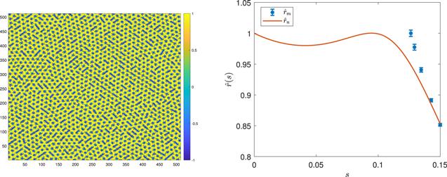
There are also cases that the ${\hat{r}}_{m}$ are not fitted very well by the theocratical predictions. In the case of d = 0.6, b = 0.15, after erasing some skyrmions, the configuration began to enter the helical phase as shown in figure 6(a). In this case, when an isolated skyrmion is created, it is not stable and will grow into stripes. If we choose the average radius near the phase transition as a baseline, that is, we choose the ${\hat{r}}_{m}$ near the phase transition as 1, the results are shown in figure 6(b). It can be seen that the ${\hat{r}}_{m}$ approaches ${\hat{r}}_{n}$.

Figure 6.

New window|Download| PPT slide
Figure 6.Compare ${\hat{r}}_{m}$ with ${\hat{r}}_{n}$ for d = 0.6, b = 0.15.


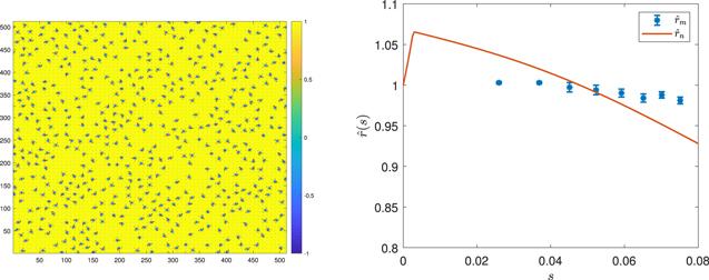
Another case is when d = 0.4, b = 0.2 as shown in figure 7. This is an example that when the skyrmions are small, they are no longer homogenously aligned. It can been found from figure 3 that the configuration is also near the phase transition from the skyrmion phase to the ferromagnetic phase. It is interesting that, the average radius is not always decreasing with s especially when s is small. For N = 51, r_s = 4.7003 ± 0.0054, for N = 103, r_s = 4.7005 ± 0.0043, which are larger than the case of a signle isolated skyrmion r_s = 4.6865. One can see that ${\hat{r}}_{n}$ has a similar behavior.

Figure 7.

New window|Download| PPT slide
Figure 7.Compare ${\hat{r}}_{m}$ with ${\hat{r}}_{n}$ for d = 0.4, b = 0.2.

4.2. A formula for the average radius in the skyrmion phase

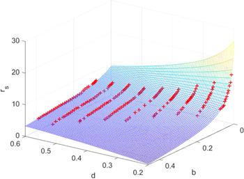
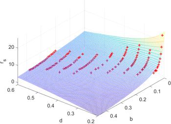
Since we start from the randomized initial state, the obtained configurations are the skyrmion lattices. In this case, the relationship between r_s, d and b are fitted by a rational function, the result is(14)$\begin{eqnarray}\begin{array}{l}{r}_{s}(d,b)\ =\displaystyle \frac{-130.88{b}^{2}+203.89{bd}-25.2503b-66.6575{d}^{2}+65.0494d+0.577576}{18.3341b+3.88567d-0.353591}.\end{array}\end{eqnarray}$r_s and fitted r_s(d, b) (equation (10)) are shown in figure 8. One can see that the rational function is consistent with the numerical results.

Figure 8.

New window|Download| PPT slide
Figure 8.r_s at different d and b (marked as ‘+') and the fitted r_s(d, b), i.e. Equation (10).


We compare equation (9) with equation (14) in figure 9. Since the ρ for each configuration is different, the results of r_s(b, d, ρ) are depicted as points in figure 9. Note that we remove the points correspond to the cases that the single isolated skyrmions are not stable such as d = 0.6, b = 0.15. It can be seen that r_s(b, d, ρ) can match the results very well. r_s(d, b, ρ) can be used to predict the average radius of the skyrmions when d, b and the density are given.

Figure 9.

New window|Download| PPT slide
Figure 9.r_s calculated with equation (9) (marked as ‘+') compared with equation (14) (the curved surface).

4.3. The shape of the skyrmion in the skyrmion phase

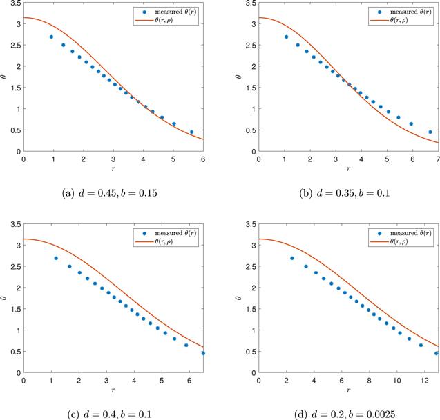
The function θ(r) is often used to describe the shape of a skyrmion [17]. It has been assumed that the higher order corrections to θ(r) are small, which in fact requires that the shape of a skyrmion is not changed significantly in the skyrmion phase. Choosing the configurations at d = 0.2, b = 0.025, d = 0.35, b = 0.1, d = 0.4, b = 0.1 and d = 0.45, b = 0.15 as examples, we measure the average θ(r) with θ in the range ${\cos }^{-1}(0.9)\leqslant \theta \leqslant {\cos }^{-1}(-0.9)$. The results are compared with θ_LO(r) with r rescaled according to $r\to r/{\hat{r}}_{f}(s)$, for example, in the case of d = 0.4, b = 0.1, one has s ≈ 0.116 165 and θ(r, ρ) = θ_LO(r/0.783516). The results are shown in figure 10.

Figure 10.

New window|Download| PPT slide
Figure 10.The shapes of isolated skyrmions in the saturated state.


As shown in figure 10, the shapes of isolated skyrmions in a saturated state are similar to the shape of a single isolated skyrmion with r rescaled. This result indicates that our assumption is valid. Note that θ(r, ρ) is also the function θ_LO(r) with b rescaled as $b/\hat{r}$. It implies that the skyrmions can be seen as being experiencing an effective magnetic strength $B^{\prime} =B/\hat{r}$ when affected by other skyrmions.

4.4. Matching

In the calculations and lattice simulations, we use dimensionless parameters. The numerical results can be matched to the real material by using the rescaling introduced in [21, 36]. The rescaling factor is denoted as q and $q\,=(D/J)\lambda /(2\pi \sqrt{2}a)$ where λ is helical wavelength and a is the lattice spacing. The helical wavelengthes of real materials can be found in [12]. For example, if we take λ ≈ 60 nm, a = 0.4 nm and D/J = 0.4, then q ≈ 6.75. Then r = 6.2854 corresponds to r = 6.2854 × q × a ≈ 16.97 nm. Meanwhile the time unit is rescaled as $t^{\prime} ={q}^{2}J{\hslash }/J^{\prime} $, where J is the dimensionless exchange strength and $J^{\prime} $ is the exchange strength of a real material. If we choose $J^{\prime} \approx 3\ \mathrm{meV}$, the time unit is $t^{\prime} \approx 0.01\ \mathrm{ns}$. The time step in the simulation is ${\rm{\Delta }}t=0.01t^{\prime} \approx 1\ \mathrm{ps}$.

5. Summary

One of the reasons that the skyrmion is proposed as a candidate for the future memory devices is because the size of a skyrmion is small. The radius of a skyrmion when the density of skyrmions is between the skyrmion lattice and the single isolated skyrmion is an important issue which is lack of exploration. In this paper, we study the average radius of skyrmions when the density is between a skyrmion lattice and a single isolated skyrmion. By using the harmonic oscillator expansion, the dependency of the average radius of skyrmions on the parameters of materials, strength of external magnetic field and the density of skyrmions is obtained theoretically. Then, a lattice simulation of LLG equation is performed to verify our results.

The theoretical result is presented in equation (9). Our result indicates that generally the average radius of skyrmions will decrease with the growth of density even when b and d are unchanged. The average radii at different d and b are measured by using lattice simulation. We confirm that our theoretical results can fit the simulated results well. With this relation, the skyrmion radius for different materials at different densities can be easily predicted. We also find that, the shapes of the skyrmions are insensitive to the density, which implies that the interactions between skyrmions can be seen as an effective magnetic strength.

Acknowledgments

This work was partially supported by the National Natural Science Foundation of China under Grant No. 12 047 570 and the Natural Science Foundation of the Liaoning Scientific Committee Grant No. 2019-BS-154.

Reference View Option By original order
By published year
By cited within times
By Impact factor

[1]Skyrme T 1962 Nucl. Phys. 31 556
DOI:10.1016/0029-5582(62)90775-7 [Cited within: 1]

[2]Bogdanov A N Yablonskii D A 1989 Sov. Phys. JETP 68 101
[Cited within: 1]

[3]Rößler U K Bogdanov A N Pfleiderer C 2006 Nature 442 797
DOI:10.1038/nature05056 [Cited within: 1]

[4]Mühlbauer S Binz B Jonietz F Pfleiderer C Rosch A Neubauer A Georgii R Böni P 2009 Science 323 915
DOI:10.1126/science.1166767

[5]Yu X Onose Y Kanazawa N Park J Han J Matsui Y Nagaosa N Tokura Y 2010 Nature 465 901
DOI:10.1038/nature09124

[6]Heinze S von Bergmann K Menzel M Brede J Kubetzka A Wiesendanger R Bihlmayer G Blügel S 2011 Nat. Phys. 7 713
DOI:10.1038/nphys2045 [Cited within: 1]

[7]Dzyaloshinsky I 1958 J. Phys. Chem. Solids 4 241
DOI:10.1016/0022-3697(58)90076-3 [Cited within: 1]

[8]Moriya T 1960 Phys. Rev. 120 91
DOI:10.1103/PhysRev.120.91 [Cited within: 1]

[9]Wang X Yuan H Wang X 2018 Commun. Phys. 1 31
DOI:10.1038/s42005-018-0029-0 [Cited within: 2]

[10]Iwasaki J Mochizuki M Nagaosa N 2013 Nat. Commun. 4 1463
DOI:10.1038/ncomms2442

[11]Fert A Reyren N Cros V 2017 Nat. Rev. Mater. 2 17031
DOI:10.1038/natrevmats.2017.31 [Cited within: 2]

[12]Nagaosa N Tokura Y 2013 Nat. Nanotechnol. 8 899
DOI:10.1038/nnano.2013.243 [Cited within: 1]

[13]Lonsky M Hoffmann A 2020 APL Mater. 8 100903
DOI:10.1063/5.0027042

[14]Leonov A O Monchesky T L Romming N Kubetzka A Bogdanov A N Wiesendanger R 2016 New J. Phys. 18 065003
DOI:10.1088/1367-2630/18/6/065003

[15]Bogdanov A N Panagopoulos C 2020 Nat. Rev. Phys. 2 492
DOI:10.1038/s42254-020-0203-7 [Cited within: 2]

[16]Bogdanov A Hubert A 1994 Phys. Status Solidi B Basic Res. 186 527
DOI:10.1002/pssb.2221860223 [Cited within: 1]

[17]Yang J-C Mao Q-Q Shi Y 2019 J. Phys. Condens. Matter. 31 165802
DOI:10.1088/1361-648x/ab01ef [Cited within: 6]

[18]Komineas S Melcher C Venakides S 2020 Nonlinearity 33 3395
DOI:10.1088/1361-6544/ab81eb [Cited within: 1]

[19]Bogdanov A Hubert A 1994 J. Magn. Magn. Mater. 138 255
DOI:10.1016/0304-8853(94)90046-9 [Cited within: 3]

[20]Yang J-C Mao Q-Q Shi Y 2019 Mod. Phys. Lett. B 33 1950040
DOI:10.1142/S0217984919500404 [Cited within: 2]

[21]Liu Y-H Li Y-Q 2013 J. Phys. Condens. Matter. 25 076005
DOI:10.1088/0953-8984/25/7/076005 [Cited within: 2]

[22]Tatara G Kohno H Shibata J 2008 Phys. Rep. 468 213
DOI:10.1016/j.physrep.2008.07.003

[23]Zang J Mostovoy M Han J H Nagaosa N 2013 J. Phys. Condens. Matter. 25 076005
DOI:10.1088/0953-8984/25/7/076005 [Cited within: 2]

[24]Iwasaki J Mochizuki M Nagaosa N 2013 Nat. Nanotech. 8 742
DOI:10.1038/nnano.2013.176 [Cited within: 1]

[25]Mochizuki M 2011 Phys. Rev. Lett. 108 017601
DOI:10.1103/PhysRevLett.108.017601 [Cited within: 2]

[26]Schütte C Iwasaki J Rosch A Nagaosa N 2014 Phys. Rev. B 90 174434
DOI:10.1103/PhysRevB.90.174434 [Cited within: 1]

[27]Koshibae W Nagaosa N 2017 Sci. Rep. 7 42645
DOI:10.1038/srep42645 [Cited within: 1]

[28]Wang C Zhai H 2017 Phys. Rev. B 96 144432
DOI:10.1103/PhysRevB.96.144432

[29]Nepal R Güngördü U Kovalev A A 2018 Appl. Phys. Lett. 112 112404
DOI:10.1063/1.5013620

[30]Sampaio J Cros V Rohart S Thiaville A Fert A 2013 Nat. Nanotechnol. 8 839
DOI:10.1038/nnano.2013.210

[31]Litzius K et al. 2017 Nat. Phys. 13 170
DOI:10.1038/nphys4000

[32]Jiang W et al. 2017 Nat. Phys. 13 162
DOI:10.1038/nphys3883

[33]Tomasello R Puliafito V Martinez E Manchon A Ricci M Carpentieri M Finocchio G 2017 J. Phys. D: Appl. Phys. 50 325302
DOI:10.1088/1361-6463/aa7a98

[34]Yang S H Ryu K S Parkin S 2015 Nat. Nanotechnol. 10 221
DOI:10.1038/nnano.2014.324

[35]Barker J Tretiakov O A 2016 Phys. Rev. Lett. 116 147203
DOI:10.1103/PhysRevLett.116.147203 [Cited within: 1]

[36]Tchoe Y Han J H 2012 Phys. Rev. B 85 174416
DOI:10.1103/PhysRevB.85.174416 [Cited within: 1]