Yu-Qi Xin, Jun-Gang Deng, Hong-Fei Zhang^,School of Nuclear Science and Technology, Lanzhou University, 730000 Lanzhou, China

Received:2021-01-7Revised:2021-04-8Accepted:2021-04-8Online:2021-04-29


Abstract
In the present work, we systematically investigate the proton radioactivity half-lives of spherical proton emitters adopting a generalized liquid drop model (GLDM) with 16 different proximity potentials, of which the proximity potential Prox.77-13 gives the closest results to the experimental data. Combined with the previous conclusion that the GLDM with proximity potential Prox.77-13 can also best describe $\alpha$ decay half-lives, which makes the model more uniform and consistent. Further, we use the proximity potential Prox.77-13 in GLDM to predict the proton radioactivity half-lives of 14 spherical proton emitters that are allowed energetically but not yet observed experimentally or specifically quantified. Finally, we research the Geiger−Nuttall law for proton radioactivity. The results reveal that the Geiger−Nuttall law can also be well used to study the proton radioactivity half-lives of isotopes with the same orbital angular momentum l.
Keywords： spherical proton emitter;GLDM;proximity energy;Geiger−Nuttall law


PDF (0KB)MetadataMetricsRelated articlesExportEndNote|Ris|BibtexFavorite
Cite this article
Yu-Qi Xin, Jun-Gang Deng, Hong-Fei Zhang. Proton radioactivity within the generalized liquid drop model with various versions of proximity potentials. Communications in Theoretical Physics, 2021, 73(6): 065301- doi:10.1088/1572-9494/abf5e6

1. Introduction

The research of exotic processes near the extremes of the nuclide chart is one of the current hot topics in nuclear physics, and proton radioactivity is one such exotic process. Since the first discovery of proton radioactivity by Jackson et al in 1970 [1], with the development and improvement of experimental facilities and radiation beams, proton radioactivity has also been observed for many nuclei with mass numbers spanning from 110 to 185 [2], with half-life length concentrated in the range of 10⁻⁶ seconds to a few seconds. Proton-rich nuclei above the proton drip line would tend to stabilize by spontaneously emitting protons, and in turn, the proton drip line inherently provides certain limiting conditions for the synthesis of proton-rich nuclei in explosive objects as well, known as rapid proton capture [3-5]. Proton radioactivity, as a typical decay mode of nuclei beyond the proton drop line, is a powerful tool for studying the properties and structures of very proton-rich nuclei [6, 7]. Thus both experimental measurements and theoretical studies of proton radioactivity are becoming increasingly necessary.

In this study, we calculate the proton radioactivity half-lives of spherical proton emitters within the generalized liquid drop model (GLDM). The GLDM takes into account the asymmetry of mass and charge, shape evolution, and proximity energy, and it is a relatively unified theory that is well able to describe and predict the half-lives of proton radioactivity, $\alpha$ decay, cluster radioactivity, spontaneous fission, and the reaction crossing section of heavy-ion fusion [8-13]. In the GLDM, when the potential barrier corresponding to the reaction process is constructed, the process can be considered as a barrier penetration problem and the WKB approximation can be used to calculate the penetration probability of the potential barrier. Besides, for proton radioactivity, the contribution of the centrifugal potential from the orbital angular momentum should be taken into account in the total energy E of the system. So far, many theoretical models have used different nuclear potentials between the emitted proton and the daughter nucleus to calculate the proton radioactive half-life, such as the Jeukenne, Lejeune, and Mahaux (JLM) effective interaction [14], the effective interaction of density-dependent M3Y (DDM3Y) [14-16], the distorted wave Born approximation [17], the Coulomb and proximity model (CPPM) [18, 19], the Gamow-like model [20, 21] and so on.

The special features of GLDM lie in two main aspects, namely the quasimolecular shape mechanism [10] and the proximity potential. The benefit of the quasimolecular shape is the ability to describe the static transition process between one and two bodies during fission or fusion. During this process, a deep and narrow neck emerges, while attractive nuclear forces remain between the nucleon on either side of the neck [10, 22-25], this is called the proximity potential, and it has a significant effect on the potential barriers. Since the proximity potential was first used in 1977 [24], many physicists have improved or proposed new proximity potentials, either by adopting a better format for the surface energy coefficients [26-32] or by going further and improving the form of the universal function [25, 33-41]. These parameters are determined from experimental data on heavy-ion reactions and given that experimental data on proton radioactivity have become more abundant since 1970. It is necessary to investigate which of the current proximity potentials can best describe the available experimental data on proton radioactivity when applied to the more uniform GLDM. A recent work [18] has shown that using the proximity potential Guo2013 to the CPPM model provides the best description of proton radioactivity data, while the GLDM [42] combined with the proximity potential Prox.77-13 gives the closest results to the $\alpha$ decay half-life data. Inspired by this, we have first systematically studied the proton radioactivity half-lives of spherical proton emitters using GLDM with different proximity potentials, compared them with experimental data, and analyzed their physical mechanism. This proximity potential is then applied to GLDM to predict the half-lives of proton radioactivity for those spherical proton emitters that are energetically permissible but not yet observed or specifically quantified experimentally. Finally, the Geiger−Nuttall law for proton radioactivity is investigated.

The paper is organized as follows: the theoretical framework for calculating the radioactive half-life of protons and the expressions for the proximity potential involved in the calculation are briefly described in section 2. The results of the calculations and the discussion are given in section 3. Finally, a summary is presented in section 4.

2. Model and method

2.1. The generalized liquid drop model

For the GLDM [8-10, 13, 22, 43], the total energy includes five parts: the volume, surface, Coulomb, proximity energies, and the additional centrifugal potential:
(1)$\begin{eqnarray}E={E}_{V}+{E}_{S}+{E}_{C}+{E}_{\mathrm{Prox}}+{E}_{l}.\end{eqnarray}$


In the one−body case, they are each given by:
(2)$\begin{eqnarray}{E}_{V}=-15.494(1-1.8{I}^{2})A,\end{eqnarray}$

(3)$\begin{eqnarray}{E}_{S}=17.9439(1-2.6{I}^{2}){A}^{2/3}(S/4\pi {R}_{0}^{2}),\end{eqnarray}$

(4)$\begin{eqnarray}{E}_{C}=0.6{e}^{2}({Z}^{2}/{R}_{0})\times 0.5\int {\left(V(\theta )/{V}_{0})(R(\theta )/{R}_{0}\right)}^{3}\sin \theta {\rm{d}}\theta ,\end{eqnarray}$
where I is the relative neutron excess and S is the surface area of the one-body nucleus. V(θ) denotes the electrostatic potential on the surface and V₀ represents the surface potential of the sphere. When transformed into two bodies:
(5)$\begin{eqnarray}{E}_{V}=-15.494[(1-1.8{I}_{1}^{2}){A}_{1}+(1-1.8{I}_{2}^{2}){A}_{2}],\end{eqnarray}$

(6)$\begin{eqnarray}{E}_{S}=17.9439[(1-2.6{I}_{1}^{2}){A}_{1}^{2/3}+(1-2.6{I}_{2}^{2}){A}_{2}^{2/3}],\end{eqnarray}$

(7)$\begin{eqnarray}{E}_{C}=0.6{e}^{2}{Z}_{1}^{2}/{R}_{1}+0.6{e}^{2}{Z}_{2}^{2}/{R}_{2}+{e}^{2}{Z}_{1}{Z}_{2}/r.\end{eqnarray}$


The centrifugal energy E_l(r) can be obtained by [44]
(8)$\begin{eqnarray}{E}_{l}=\displaystyle \frac{{{\hslash }}^{2}{\left(l+1/2\right)}^{2}}{2\mu {r}^{2}}.\end{eqnarray}$
Here A_i, Z_i, R_i, and I_i are the mass numbers, proton numbers, radii, and the relative neutron excesses of proton and daughter nucleus, respectively. Should note that the I₂ of the proton is set to 0 to ensure a positive and a negative volume and surface energy. And l is the angular momentum carried away by the emitted proton. The calculation is done using its minimum value [45], which is given by observing the spin−parity conservation laws. The radius of proton radioactivity decay parent nucleus, daughter nucleus, and the emitted proton can be obtained by
(9)$\begin{eqnarray}{R}_{i}=1.28{A}_{i}^{1/3}-0.76+0.8{A}_{i}^{-1/3}(i=0,1,2).\end{eqnarray}$


The half-life of a spherical proton emitter is defined as $\nu P=\mathrm{ln}2/{T}_{1/2}$. The assault frequency ν is given by
(10)$\begin{eqnarray}\nu =\displaystyle \frac{1}{2{R}_{0}}\sqrt{\displaystyle \frac{2{E}_{p}}{{M}_{p}}},\end{eqnarray}$
here, E_p and M_p are the kinetic energy and mass of the emitted proton. The barrier penetrating probability P can be obtained by the following formula
(11)$\begin{eqnarray}P=\exp \left[-\displaystyle \frac{2}{{\hslash }}{\int }_{{r}_{\mathrm{in}}}^{{r}_{\mathrm{out}}}\sqrt{2B(r)({E}_{r}-E(\mathrm{sphere}))}{\rm{d}}r\right],\end{eqnarray}$
where r denotes the distance between the centers of the emitted proton and of the daughter nucleus. The classical two turning points r_in and r_out are calculated by: r_in = R₁ + R₂ and E(r_out) = Q_p. B(r) = $\mu$ denotes the reduced mass between the emitted proton and daughter nucleus.

2.2. The proximity energy

As covered in the introductory section, when a deep and narrow neck occurs during fission or fusion, the nuclear forces, or proximity energies, between nucleon close together on either side of the neck need to be considered. The proximity energy is defined as the product of a factor concerning the average curvature of the interaction surfaces and a universal function with respect to the separation distance [18, 33]. In this study, a total of 16 proximity potentials are chosen to replace the original proximity potential in the GLDM to calculate the proton radioactivity half-lives, namely: proximity potential Prox.77 [24] and its 12 improved versions [26-32, 46], Bass80 [41], Prox.81 [25], and Guo2013 [34].

2.2.1. The proximity potential Prox.77

The proximity energy Prox.77 [24] are expressed as,
(12)$\begin{eqnarray}{E}_{\mathrm{Prox}}(r)=4\pi \gamma b\bar{R}\phi (\xi ),\end{eqnarray}$
here, the mean curvature radius $\bar{R}$ can be calculated with
(13)$\begin{eqnarray}\bar{R}=\displaystyle \frac{{C}_{1}{C}_{2}}{{C}_{1}+{C}_{2}},\end{eqnarray}$
where C₁ and C₂ represent the matter radii of proton and daughter nucleus, respectively. These two cofficients are given by
(14)$\begin{eqnarray}{C}_{i}={R}_{i}\left[1-{\left(\displaystyle \frac{b}{{R}_{i}}\right)}^{2}\right](i=1,2),\end{eqnarray}$
with the effective sharp radius R_i calculating by equation (9).

γ is the surface energy coefficient:
(15)$\begin{eqnarray}\gamma ={\gamma }_{0}(1-{k}_{s}{A}_{s}^{2}),\end{eqnarray}$
where, A_s = (N − Z)/A is the neutron-proton excess. The improved versions of the proximity potential Prox.77 have only had its surface energy constant γ₀ and the surface asymmetry constant k_s adjusted accordingly:Prox.77-1: γ₀ = 0.9517 (MeV fm⁻²), k_s = 1.7826 [24]
Prox.77-2: γ₀ = 1.017 34 (MeV fm⁻²), k_s = 1.79 [26]
Prox.77-3: γ₀ = 1.460 734 (MeV fm⁻²), k_s = 4.0 [27]
Prox.77-4: γ₀ = 1.2402 (MeV fm⁻²), k_s = 3.0 [28]
Prox.77-5: γ₀ = 1.1756 (MeV fm⁻²), k_s = 2.2 [29]
Prox.77-6: γ₀ = 1.273 26 (MeV fm⁻²), k_s = 2.5 [29]
Prox.77-7: γ₀ = 1.2502 (MeV fm⁻²), k_s = 2.4 [29]
Prox.77-8: γ₀ = 0.9517 (MeV fm⁻²), k_s = 2.6 [47]
Prox.77-9: γ₀ = 1.2496 (MeV fm⁻²), k_s = 2.3 [30]
Prox.77-10: γ₀ = 1.252 84 (MeV fm⁻²), k_s = 2.345 [31]
Prox.77-11: γ₀ = 1.089 48 (MeV fm⁻²), k_s = 1.9830 [32]
Prox.77-12: γ₀ = 0.9180 (MeV fm⁻²), k_s = 0.7546 [32]
Prox.77-13: γ₀ = 0.911 445 (MeV fm⁻²), k_s = 2.2938 [32]
The universal function φ(ξ) is written as
(16)$\begin{eqnarray}\begin{array}{l}\phi (\xi )\\ =\left\{\begin{array}{ll}-\displaystyle \frac{1}{2}{\left(\xi -{\xi }_{0}\right)}^{2}-0.0852{\left(\xi -{\xi }_{0}\right)}^{3}, & 0\lt \xi \leqslant 1.2511,\\ -3.347\exp (\displaystyle \frac{-\xi }{0.75}), & \xi \geqslant 1.2511,\end{array}\right.\end{array}\end{eqnarray}$
where ξ₀ = 2.54. ξ = (r − C₁ − C₂)/b represents the distance between the near surface of the daughter nucleus and the emitted proton with the width coefficient b fixed to a unity value.

2.2.2. The proximity potential Prox.81

The form of the proximity energy Prox.81 [25] is very similar to that of the proximity energy Prox.77 but the universal function φ(ξ) in it has a different expression than that of Prox.77:
(17)$\begin{eqnarray}\begin{array}{l}\phi (\xi )\,=\,\left\{\begin{array}{ll}-4.41{{\rm{e}}}^{-\xi /0.7176}, & \xi \geqslant 1.9475,\\ -1.7817\,+\,0.927\xi +0.01696{\xi }^{2}-0.05148{\xi }^{3}, & 0\lt \xi \lt 1.9475,\\ -1.7817\,+\,0.927\xi +0.143{\xi }^{2}-0.09{\xi }^{3}, & \xi \leqslant 0,\end{array}\right.\end{array}\end{eqnarray}$
here γ₀ = 0.9517 (MeV/fm²), k_s = 1.7826.

2.2.3. The proximity potential Bass80

Bass (1977, 1980) [41] derived a potential using a geometric interpretation of fusion data above the barrier for systems with Z₁Z₂ = 64 − 850:
(18)$\begin{eqnarray}{E}_{\mathrm{Prox}}(r)=-\bar{R}{[0.033\exp (\xi /3.5)+0.007\exp (\xi /0.65)]}^{-1},\end{eqnarray}$
where ξ and $\bar{R}$ take the same form as before, but here ${C}_{i}={R}_{i}\left(1-\tfrac{0.98}{{{R}_{i}}^{2}}\right)$.

3. Results and discussion

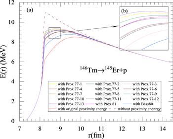
Since this work requires the application of different proximity potentials to the GLDM, these proximity potentials should first meet certain conditions in order to be self-consistent with the GLDM. This means that the radius equations for these proximity potentials should be consistent with those in the framework of the GLDM and that the total potential curves constructed should be reasonable. We, therefore, chose 16 proximity potentials that satisfy the above conditions and applied them to the GLDM to investigate which of the calculated proton radioactivity half-lives gives the lowest root-mean-square (RMS) value compared to the experimental data. These are the proximity potential Prox.77-1 [24] and its 12 improved versions Prox.77-2-13 [26-32, 47] obtained by improving the corresponding surface energy coefficients, as well as the proximity potentials Bass80 [41], Prox.81 [25] and Guo2013 [34], which are obtained by improving the universal functions. In the specific calculation, it should be the same problem as the one encountered in Deng’s article [42] that the proximity potential Guo2013 cannot be applied in GLDM. For example, in figure 1, the potential barrier curves for ¹⁴⁶Tm when applying different proximity potentials in GLDM are given. In the region shown in figure 1(a), the barrier corresponding to the proximity potential Guo2013 drops abruptly to −7.5 MeV from 8.1 fm and then increases smoothly until 12 fm, until the curve coincides with other proximity potential curves. The graph also shows that for ¹⁴⁶Tm the effect of the proximity potential on the barrier curve is almost exclusively between 8 and 12 fm, as the rest range of the curve coincides almost exactly. So it can be attributed that the proximity potential Guo2013 gives an attractive effect that is too strong.

Figure 1.

New window|Download| PPT slide
Figure 1.Total potential barrier curves for ¹⁴⁶Tm when using different proximity potentials in GLDM.


The experimental proton radioactive half-lives, spin, parity, and Q_p used in this work are all taken from the recently evaluated atomic mass table AME2016 [47, 48] and the nuclear properties table NUBASE2016 [49]. We calculated the RMS values $\sigma =\sqrt{\sum {\left({\mathrm{log}}_{10}{T}_{1/2}^{{\rm{th}}}-{\mathrm{log}}_{10}{T}_{1/2}^{{\rm{\exp }}}\right)}^{2}/n}$ between the calculated proton radioactivity half-lives using GLDM with different proximity potentials and the experimental data for 27 spherical proton emitters ranging in proton number between 69 and 83, and the relevant results are presented in table 1. As can be seen in this table, the differences between the calculated results are not particularly large. The proximity potential Prox.77-13 gives the closest results to the experimental data, while the original version, gives the largest deviation from the experimental data. The proximity potential Prox.77-13, when applied to the GLDM, improves the original version by 5.71%, which is not a large improvement, but firstly based on the relatively small amount of experimental data on proton radioactivity itself, and secondly, the effect of the proximity potential on the total potential barrier is only in the small range of 3-4 fm, this result is still of some significance. This, coupled with the recent work by Deng et al [42] that the most suitable proximity potential for the calculation of $\alpha$ decay within GLDM is also Prox.77-13, suggests that the results of our work are more coherent and general.


Table 1.
Table 1.The second column denotes the RMS deviations between logarithmic calculated proton radioactivity half-lives by GLDM with different proximity potentials and experimental data. The last column denotes the logarithmic values of proton radioactivity half-lives of ¹⁴⁶Tm calculated by GLDM with different proximity potentials. The half-lives are in units of 's’.

GLDM with proximity potential	σ	${\mathrm{log}}_{10}{T}_{1/2}^{{}^{146}{\rm{Tm}}}$
Prox.77-1	0.6646	−0.747 35
Prox.77-2	0.6663	−0.751 23
Prox.77-3	0.6774	−0.777 33
Prox.77-4	0.6718	−0.764 27
Prox.77-5	0.6703	−0.760 57
Prox.77-6	0.6728	−0.766 37
Prox.77-7	0.6722	−0.765 00
Prox.77-8	0.6645	−0.747 21
Prox.77-9	0.6722	−0.764 99
Prox.77-10	0.6723	−0.765 18
Prox.77-11	0.6681	−0.755 48
Prox.77-12	0.6639	−0.745 53
Prox.77-13	0.6635	−0.744 90
Prox.81	0.6652	−0.750 41
Bass80	0.6814	−0.786 00
Original one	0.7037	−0.833 77

New window|CSV

Next, we explore what makes them differ from each other in terms of results. From the previous section 2, it is clear that the half-life is only related to two factors, the assault frequency ν and the penetrating probability P, while ν is fixed for the same nucleus. From the formula for calculating P, it is clear that it is only related to r_in, r_out, and the shape of the total potential barrier. From the formulas for r_in and r_out, we know that these two values are also fixed, thus the difference between the calculated proton radioactivity half-lives is due to the different total GLDM energy. Take ¹⁴⁶Tm as an example, we list in the last column of table 1 the logarithmic values of the proton radioactivity half-lives of ¹⁴⁶Tm obtained when the different proximity potentials are applied to the GLDM, and the relevant area in figure 1(a) is shown enlarged in figure 1(b). Firstly, we can see that the proximity potential makes the height of the barrier decrease and the position of the peak point change. Secondly, we see that the purple curve represents the highest total barrier curve corresponding to the proximity potential Prox.77-13, resulting in the longest half-life, while the red curve represents the lowest total barrier curve corresponding to the original proximity potential, resulting in the shortest half-life.

Subsequently, we present the experimental data and the best and worst results compared to the experimental data in table 2. The first and second columns represent the parent nuclei and daughter nuclei, respectively, and the two immediately following columns represent their corresponding spin/parity. The fifth column shows the decay energies. The sixth column represents the minimum angular momentum carried away by the emitted protons. The seventh column represents the experimental proton radioactivity half-lives, and the last two columns are the proton radioactivity half-lives calculated by GLDM using the proximity potential Prox.77-13 and the original version, respectively, labeled as ${\mathrm{log}}_{10}{T}_{1/2}^{77-13}$ and ${\mathrm{log}}_{10}{T}_{1/2}^{\mathrm{Ori}}$. Among them, the parent nucleus ^146mTm decays to ¹⁴⁵Er accompanied by ${l}_{\min }=5$. If it follows the binding energy and spin/parity of ^145mEr given in NUBASE2016 [49], i.e. ^146mTm decays to ^145mEr, with Q_p = 1.001MeV, ${l}_{\min }=0$ and the corresponding proton radioactivity half-life is calculated to be ${\mathrm{log}}_{10}{T}_{1/2}=-2.5$ (here and below T_1/2 is in units of 's’); whereas if it decays to ¹⁴⁵Er, the corresponding result ${\mathrm{log}}_{10}{T}_{1/2}=-1.365$ is closer to the experimental datum; combined with [50], which gives the same ${l}_{\min }=5$, Q_p is also closer compared to when decays to ^145mEr. For nucleus ^150mLu, the uncertain spin/parity is given in NUBASE2016 [49]. If 1⁺ state is regarded as the spin/parity of the proton emitter, its ${l}_{\min }$ is equal to zero, and the calculated half-life is ${\mathrm{log}}_{10}{T}_{1/2}=-5.45$. However, we find that if we treat it as a 2⁺ state, although ${l}_{\min }$ increases to 2, the half-life given is closer to the experimental datum. Also, in combination with [50], we find that it has the same Q_p and ${l}_{\min }=2$ as the experimental data. So the conclusion is that the spin/parity of the nucleus ^150mLu maybe 2⁺.


Table 2.
Table 2.The logarithmic values of the proton radioactive half-lives derived when the proximity potential Prox.77-13 is applied to the GLDM, together with the corresponding results when the original version of the proximity potential is used. Elements with upper prefixes 'm'and 'n'represent the order of the excited isomeric states. '()'denotes the spin and/or parity is indeterminate. '#'means these values are estimated from the tendency of neighboring nuclides having the same Z and N parities. The experimental half-lives, spin/parity, and the proton radioactivity energies of the spherical proton emitters are taken from the NUBASE2016 [49]. All proton radioactivity half-lives and energies are in units of 's'and 'MeV’.

Proton	Daughter	${j}_{p}^{\pi }$	${j}_{d}^{\pi }$	Qp	${l}_{\min }$	${\mathrm{log}}_{10}{T}_{1/2}^{\exp }$	${\mathrm{log}}_{10}{T}_{1/2}^{77-13}$	${\mathrm{log}}_{10}{T}_{1/2}^{\mathrm{Ori}}$
145Tm	144Er	(11/2−)	0+	1.741	5	−5.498 94	−6.024 20	−6.088 03
146Tm	145Er	(1+)	1/2+#	0.891	0	−0.809 67	−0.744 90	−0.833 77
146mTm	145Er	(5−)	1/2+#	l.201	5	−1.124 94	−1.365 37	−1.429 20
147Tm	146Er	11/2−	0+	1.059	5	0.572 87	0.406 40	0.341 77
147mTm	146Er	3/2+	0+	1.120	2	−3.443 70	−3.322 00	−3.405 65
150mLu	149Yb	(1+, 2+)	(1/2+)	1.291	2	−4.397 94	−4.683 97	−4.762 38
151mLu	150Yb	(3/2+)	0+	1.291	2	−4.782 52	−4.693 05	−4.772 86
155Ta	154Hf	(11/2−)	0+	1.451	5	−2.494 85	−2.930 10	−2.989 59
156Ta	155Hf	(2−)	7/2−#	1.021	2	−0.826 81	−0.726 51	−0.802 13
156mTa	155Hf	(9+)	7/2−#	1.111	5	0.923 76	0.830 10	0.770 23
157Ta	156Hf	1/2+	0+	0.941	0	−0.528 71	−0.211 58	−0.294 78
160Re	159W	(4−)	7/2−#	1.271	0	−3.163 68	−4.121 50	−4.199 74
161Re	160W	1/2+	0+	1.201	0	−3.356 55	−3.310 40	−3.389 68
161mRe	160W	11/2−	0+	1.321	5	−0.679 85	−1.174 20	−1.232 43
165mIr	164Os	(11/2−)	0+	1.721	5	−3.429 46	−4.294 27	−4.350 21
166Ir	165Os	(2−)	(7/2−)	1.161	2	−0.841 64	−1.484 46	−1.554 32
166mIr	165Os	(9+)	(7/2−)	1.331	5	−0.090 44	−0.792 18	−0.848 35
167Ir	166Os	1/2+	0+	1.071	0	−1.127 84	−0.965 68	−1.042 01
167mIr	166Os	11/2−	0+	1.246	5	0.778 15	0.175 67	0.118 72
170Au	169Pt	(2−)	(7/2−)	1.471	2	−3.488 12	−4.386 11	−4.452 73
170mAu	169Pt	(9+)	(7/2−)	1.751	5	−2.974 69	−4.109 69	−4.163 58
171Au	170Pt	(1/2+)	0+	1.448	0	−4.651 70	−4.879 26	−4.952 22
171mAu	170Pt	11/2−	0+	1.702	5	−2.586 70	−3.740 66	−3.795 34
176Tl	175Hg	(3−, 4−, 5−)	(7/2−)	1.261	0	−2.207 61	−2.306 56	−2.375 19
177Tl	176Hg	(1/2+)	0+	1.155	0	−1.178 49	−0.929 37	−0.998 74
177mTl	176Hg	(11/2−)	0+	1.962	5	−3.459 67	−5.190 03	−5.246 75
185mBi	184Pb	1/2+	0+	1.607	0	−4.191 79	−5.352 62	−5.423 39

New window|CSV

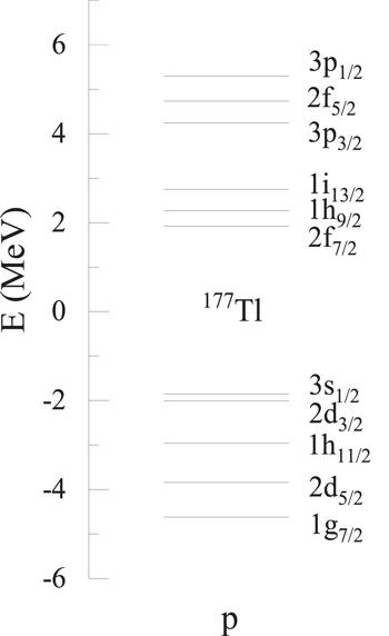
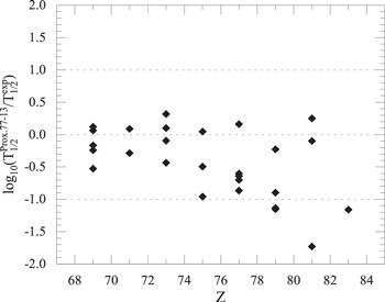
From table 2, we can see that the half-life calculated for ^177mTl is more than one order of magnitude smaller than the experimental value. Moreover, we note that the spin/parity of the parent nucleus is uncertain, and if the value of ${l}_{\min }$ increases, the half-life length will be significantly longer. If we take ${l}_{\min }=6$, the final result is ${\mathrm{log}}_{10}{T}_{1/2}=-4.01366$, which is closer to the experimental value, that is, the spin/parity of the parent nucleus should be 13/2⁺. However, this conclusion is unreasonable, as we present in figure 2 the spherical single-particle energy levels corresponding to the protons of ¹⁷⁷Tl obtained by using the WS* parameters [51-53]. From the figure, we can see that the energy level 1i_13/2, which corresponds to 13/2⁺, is above the main shell Z = 82, and its position is much higher than the position of 3s_1/2 in the ground state. The difference in energy between ¹⁷⁷Tl and ^177mTl is calculated by the AME2016 mass table [47, 48] to be only 807 KeV, which clearly shows that the spin/parity of ^177mTl should be wrong at 13/2⁺. The reason for such a large difference may originate from microscopic effects. Subsequently, we realized that the spectroscopic factor [54-56] ${S}_{p}={u}_{j}^{2}$ is also important for calculating the proton radioactivity, where u²_j represents the probability that the spherical orbit of the emitted proton is empty in the corresponding daughter nucleus. The spectroscopic factors are quite important from the viewpoint of nuclear structure. Since the proton is a quasiparticle in the nuclear volume, however, the previous results were only based on calculations with 'pure'potential, so the results should be corrected by the spectroscopic factors. It is also noted that the spectroscopic factors calculated from the relativistic mean field theory combined with the BCS method in [56] have been successfully applied to the GLDM to calculate the proton radioactivity half-lives. If the spectroscopic factor S_p = 0.022 for nucleus ^177mTl from [56] is used and substituted into the equation ${S}_{p}P\nu =\mathrm{ln}2/{T}_{1/2}$, where both ν and P are calculated in this work, the final result of the proton radioactive half-life can be found to be ${\mathrm{log}}_{10}{T}_{1/2}=-3.53$, which is very close to the experimental value of ${\mathrm{log}}_{10}{T}_{1/2}=-3.46$. We then plotted the logarithmic difference between ${\mathrm{log}}_{10}{T}_{1/2}^{77-13}$ and ${\mathrm{log}}_{10}{T}_{1/2}^{\mathrm{Ori}}$ in figure 3. From this picture, it is clear that the deviation between the theoretical and experimental half-lives tends to become larger near the proton number 82, which may be attributed to the shell effect that becomes apparent as Z approaches 82.

Figure 2.

New window|Download| PPT slide
Figure 2.The spherical single-particle levels of the proton of ¹⁷⁷Tl using WS* parameters [51-53].

Figure 3.

New window|Download| PPT slide
Figure 3.The logarithmic differences between ${\mathrm{log}}_{10}{T}_{1/2}^{{\rm{77-13}}}$ and ${\mathrm{log}}_{10}{T}_{1/2}^{{\rm{\exp }}}$.


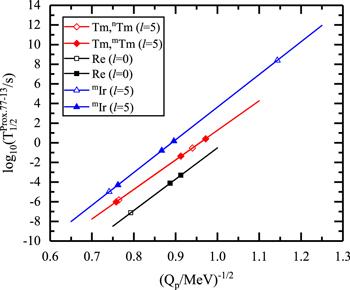
Further, we applied the proximity potential Prox.77-13 to the GLDM to predict the proton decay half-lives of 14 spherical proton emitters, where all 14 nuclei are energetically allowed in NUBASE2016 [49] but not yet observed experimentally or specifically quantified. The predicted calculations are listed in table 3, where the first six columns are all the same as those indicated in table 2. The last column shows the predicted half-lives of proton radioactivity, labeled as ${\mathrm{log}}_{10}{T}_{1/2}^{77-13}$. Much works have been done on natural $\alpha$ radioactivity since the beginning of the last century, and Geiger and Nuttall [57] found a correlation between decay energy and decay half-lives. For $\alpha$ decay, there has been recent work [58] that makes important development to the original Geiger−Nuttall law by adding terms to the law. Meanwhile, many studies [18, 45, 59-61] have shown that the Geiger−Nuttall law can also apply to describe the proton radioactivity isotopes with the same ${l}_{\min }$. In addition, Ren et al [62] have recently developed a new formula to reproduce the half-lives of cluster radioactivity, extending the Geiger−Nuttall law from simple $\alpha$ decay to complex cluster radioactivity. In the present work, we plot the calculated logarithmic half-lives ${\mathrm{log}}_{10}{T}_{1/2}^{77-13}$ against ${Q}_{p}^{-1/2}$ for Tm, Re, and Ir isotopes in figure 4, where each kind of isotopes have the same angular momentum ${l}_{\min }$. The solid symbols indicate the ${\mathrm{log}}_{10}{T}_{1/2}^{77-13}$ from table 2, while the open symbols indicate the ${\mathrm{log}}_{10}{T}_{1/2}^{77-13}$ predicted from table 3. In this figure, a good linear relationship is maintained between ${\mathrm{log}}_{10}{T}_{1/2}^{77-13}$ and ${Q}_{p}^{-1/2}$ for each isotopes. In particular, as many as five nuclei in each of the Tm and Ir isotopes are perfectly in a straight line, including the predicted results represented by the open symbols, which further proves the credibility of our calculations. This reveals that the Geiger−Nuttall law is a good guide for both theoretical calculations and experimental discrimination of proton radioactivity half-lives.


Table 3.
Table 3.Same as table 2, but for predicted radioactivity half-lives of spherical proton emitters, whose proton radioactivity are energetically allowed in NUBASE2016 [49] but not yet observed experimentally or not yet specifically quantified, using GLDM with the proximity potential Prox.77-13.

Proton	Daughter	${j}_{p}^{\pi }$	${j}_{d}^{\pi }$	Qp	${l}_{\min }$	${\mathrm{log}}_{10}{T}_{1/2}^{77-13}$
144Tm	143Er	(10+)	9/2−#	1.711	5	−5.821 49
146nTm	145mEr	(10+)	11/2−#	1.131	5	−0.531 52
150Lu	149Yb	(5−, 6−)	(1/2+)	1.271	5	−1.623 98
151Lu	150Yb	(11/2−)	0+	1.241	5	−1.304 93
159Re	158W	1/2+#	0+	1.591	0	−7.129 46
159mRe	158W	11/2−	0+	1.801	5	−5.255 31
164Ir	163Os	2−#	7/2−	1.561	2	−5.673 61
164mIr	163Os	(9+)	7/2−	1.821	5	−4.994 51
165Ir	164Os	1/2+#	0+	1.541	0	−6.233 44
169mIr	168Os	(11/2−)	0+	0.765	5	8.389 62
169Au	168Pt	1/2+#	0+	1.931	0	−8.602 79
172Au	171Pt	(2−)	7/2−	0.861	2	4.143 58
185nBi	184Pb	13/2+#	0+	1.703	6	−1.751 81
185Bi	184Pb	9/2−#	0+	1.523	5	−1.345 77

New window|CSV

Figure 4.

New window|Download| PPT slide
Figure 4.The Geiger−Nuttall law for different cases of proton radioactivity between ${\mathrm{log}}_{10}{T}_{1/2}^{77-13}$ and ${Q}_{p}^{-1/2}$. The solid symbols indicate the ${\mathrm{log}}_{10}{T}_{1/2}^{77-13}$ from table 2, while the open symbols indicate the ${\mathrm{log}}_{10}{T}_{1/2}^{77-13}$ predicted from table 3.

4. Summary

In summary, with the development of proximity potentials and abundance of experimental data on proton radioactivity, it has become increasingly important at this stage to find the most suitable proximity potential type within the GLDM to describe and predict proton radioactivity half-lives more precisely. It is found that GLDM with the proximity potential Prox.77-13 gives the lowest RMS deviation in reproducing the proton radioactivity half-lives data of spherical proton emitters, and the combination also can give the closest results to the experimental $\alpha$ half-lives, making the model more uniform and consistent. In the calculation, we find that the ^146mTm proton radioactivity corresponds to a ¹⁴⁵Er final state that is closer to the experimental data than to the ^145mEr state, and the angular momentum carried away by the proton also matches the experimental value; the spin/parity of the ^150mLu state is uncertain, which is suggested to be the 2⁺ state instead of the 1⁺ state by our calculation results; the proton spherical single-particle levels of the ¹⁷⁷Tl indicate that the angular momentum carried by the proton during the proton radioactivity of the ^177mTl is 5 and cannot be equal to 6, these theoretical results may provide some guidance for experimentation. Finally, we use the proximity potential Prox.77-13 within the GLDM to predict the proton radioactivity half-lives and investigate the Geiger−Nuttall law for proton radioactivity. The theoretically calculated ${\mathrm{log}}_{10}{T}_{1/2}^{77-13}$ and ${Q}_{p}^{-1/2}$ of the isotopes are found to maintain a very good linear relationship, including the predicted values, thus further enhancing the reliability of the predictions. These imply that the Geiger−Nuttall law can also be employed to describe the proton radioactivity half-lives of isotopes with the same angular momentum. After completing this work, we note that the spectroscopic factor is relatively important for improving the accuracy and predictive reliability of the proton radioactivity half-life calculations. Therefore, as an outlook, it is interesting to take the spectroscopic factor into account in our model, and this work is in progress.

Acknowledgments

This work is supported by National Natural Science Foundation of China (Grants No. 11 675 066, No. 11 665 019, and No. 11 947 229), the China Postdoctoral Science Foundation (No. 2019M663853), by the Fundamental Research Funds for the Central Universities (Grants No. lzujbky-2017-ot04, and No. lzujbky-2020-it01), and Feitian Scholar Project of Gansu province.

Reference View Option By original order
By published year
By cited within times
By Impact factor

[1]Jackson K P et al. 1970 Phys. Lett. B 33 281
DOI:10.1016/0370-2693(70)90269-8 [Cited within: 1]

[2]Sonzogni A A 2002 Nucl. Data Sheets 95 1
DOI:10.1006/ndsh.2002.0001 [Cited within: 1]

[3]Schatz H et al. 1998 Phys. Rep. 294 167
DOI:10.1016/S0370-1573(97)00048-3 [Cited within: 1]

[4]Wanajo S 2006 Astrophys. J. 647 1323
DOI:10.1086/505483

[5]Wallace R K, Woosley S E 1981 Astrophys. J. Suppl. Ser. 45 389
DOI:10.1086/190717 [Cited within: 1]

[6]Karny M et al. 2008 Phys. Lett. B 664 52
DOI:10.1016/j.physletb.2008.04.056 [Cited within: 1]

[7]Kruppa A T, Nazarewicz W 2004 Phys. Rev. C 69 054311
DOI:10.1103/PhysRevC.69.054311 [Cited within: 1]

[8]Zhang H F, Zuo W, Li J Q, Royer G 2006 Phys. Rev. C 74 017304
DOI:10.1103/PhysRevC.74.017304 [Cited within: 2]

[9]Zhang H F, Royer G 2007 Phys. Rev. C 76 047304
DOI:10.1103/PhysRevC.76.047304

[10]Royer G 2000 J. Phys. G: Nucl. Part. Phys. 26 1149
DOI:10.1088/0954-3899/26/8/305 [Cited within: 3]

[11]Royer G, Zbiri K, Bonilla C 2004 Nucl. Phys. A 730 355
DOI:10.1016/j.nuclphysa.2003.11.010

[12]Bao X J et al. 2012 J. Phys. G:Nucl. Part. Phys. 39 095103
DOI:10.1088/0954-3899/39/9/095103

[13]Wang Y Z, Zhang H F, Dong J M, Royer G 2009 Phys. Rev. C 79 014316
DOI:10.1103/PhysRevC.79.014316 [Cited within: 2]

[14]Bhattacharya M, Gangopadhyay G 2007 Phys. Lett. B 651 263
DOI:10.1016/j.physletb.2007.06.012 [Cited within: 2]

[15]Basu D N, Roy Chowdhury P, Samanta C 2005 Phys. Rev. C 72 051601 (R)
DOI:10.1103/PhysRevC.72.051601

[16]Qian Y B, Ren Z Z, Ni D D 2010 Chin. Phys. Lett. 27 072301
DOI:10.1088/0256-307X/27/3/030508 [Cited within: 1]

[17]Åberg S, Semmes P B, Nazarewicz W 1997 Phys. Rev. C 56 1762
DOI:10.1103/PhysRevC.56.1762 [Cited within: 1]

[18]Deng J G, Li X H, Chen J L 2019 Eur. Phys. J. A 55 58
DOI:10.1140/epja/i2019-12728-0 [Cited within: 4]

[19]Santhosh K P, Sukumaran I 2017 Phys. Rev. C 96 034619
DOI:10.1103/PhysRevC.96.034619 [Cited within: 1]

[20]Zdeb A et al. 2016 Eur. Phys. J. A 52 323
DOI:10.1140/epja/i2016-16323-7 [Cited within: 1]

[21]Chen J L et al. 2019 J. Phys. G:Nucl. Part. Phys. 46 065107
DOI:10.1088/1361-6471/ab1a56 [Cited within: 1]

[22]Bao X J et al. 2014 Nucl. Phys. A 921 85
DOI:10.1016/j.nuclphysa.2013.11.002 [Cited within: 2]

[23]Zhang H F et al. 2014 Phys. Rev. C 90 054313
DOI:10.1103/PhysRevC.90.054313

[24]Blocki J et al. 1977 Ann. Phys. 105 427
DOI:10.1016/0003-4916(77)90249-4 [Cited within: 5]

[25]Blocki J, Świaţecki W J 1981 Ann. Phys. 132 53
DOI:10.1016/0003-4916(81)90268-2 [Cited within: 5]

[26]Myers W D, Swiatecki W J 1966 Nucl. Phys. 81 1
DOI:10.1016/0029-5582(66)90639-0 [Cited within: 4]

[27]Möller P, Nix J R 1976 Nucl. Phys. A 272 502
DOI:10.1016/0375-9474(76)90345-6 [Cited within: 1]

[28]Krappe H J, Nix J R, Sierk A J 1979 Phys. Rev. C 20 992
DOI:10.1103/PhysRevC.20.992 [Cited within: 1]

[29]Möller P, Nix J R 1981 Nucl. Phys. A 361 117
DOI:10.1016/0375-9474(81)90473-5 [Cited within: 3]

[30]Möller P, Nix J R 1988 At. Data Nucl. Data Tables 39 213
DOI:10.1016/0092-640X(88)90022-8 [Cited within: 1]

[31]Möller P et al. 1995 At. Data Nucl. Data Tables 59 185
DOI:10.1006/adnd.1995.1002 [Cited within: 1]

[32]Pomorski K, Dudek J 2003 Phys. Rev. C 67 044316
DOI:10.1103/PhysRevC.67.044316 [Cited within: 6]

[33]Dutt I, Puri R K 2010 Phys. Rev. C 81 044615
DOI:10.1103/PhysRevC.81.044615 [Cited within: 2]

[34]Guo C L, Zhang G L, Le X Y 2013 Nucl. Phys. A 897 54
DOI:10.1016/j.nuclphysa.2012.10.003 [Cited within: 2]

[35]Myers W D, Świaţecki W J 2000 Phys. Rev. C 62 044610
DOI:10.1103/PhysRevC.62.044610

[36]Dutt I, Bansal R 2010 Chin. Phys. Lett. 27 112402
DOI:10.1088/0256-307X/27/11/112402

[37]Dutt I 2011 Pramana 76 921
DOI:10.1007/s12043-011-0094-3

[38]Bass R 1973 Phys. Lett. B 47 139
DOI:10.1016/0370-2693(73)90590-X

[39]Bass R 1974 Nucl. Phys. A 231 45
DOI:10.1016/0375-9474(74)90292-9

[40]Bass R 1977 Phys. Rev. Lett. 39 265
DOI:10.1103/PhysRevLett.39.265

[41]Reisdorf W 1994 J. Phys. G: Nucl. Part. Phys. 20 1297
DOI:10.1088/0954-3899/20/9/004 [Cited within: 4]

[42]Deng J G, Zhang H F 2021 Chin. Phys. C 45 024104
DOI:10.1088/1674-1137/abcc5a [Cited within: 3]

[43]Zhang H F, Royer G 2008 Phys. Rev. C 77 054318
DOI:10.1103/PhysRevC.77.054318 [Cited within: 1]

[44]Morehead J J 1995 J. Math. Phys.J. Math. Phys. 36 5431
DOI:10.1063/1.531270 [Cited within: 1]

[45]Chen J L et al. 2019 Eur. Phys. J. A 55 214
DOI:10.1140/epja/i2019-12927-7 [Cited within: 2]

[46]Royer G, Remaud B 1984 J. Phys. G: Nucl. Phys. 10 1057
DOI:10.1088/0305-4616/10/8/011 [Cited within: 1]

[47]Huang W J et al. 2017 Chin. Phys. C 41 030002
DOI:10.1088/1674-1137/41/3/030002 [Cited within: 4]

[48]Wang M et al. 2017 Chin. Phys. C 41 030003
DOI:10.1088/1674-1137/41/3/030003 [Cited within: 2]

[49]Audi G et al. 2017 Chin. Phys. C 41 030001
DOI:10.1088/1674-1137/41/3/030001 [Cited within: 6]

[50]Blank B, Borge M J G 2008 Prog. Part. Nucl .Phys. 60 403
DOI:10.1016/j.ppnp.2007.12.001 [Cited within: 2]

[51]Wang N, Liang Z Y, Liu M, Wu X Z 2010 Phys. Rev. C 82 044304
DOI:10.1103/PhysRevC.82.044304 [Cited within: 2]

[52]Cwiok S et al. 1987 Comput. Phys. Commun. 46 379
DOI:10.1016/0010-4655(87)90093-2

[53]Damgaard J, Pauli H C, Pashkevich V V, Strutinsky V M 1969 Nucl. Phys. A 135 432
DOI:10.1016/0375-9474(69)90174-2 [Cited within: 2]

[54]Zhang Z X, Dong J M 2018 Chin. Phys. C 42 014104
DOI:10.1088/1674-1137/42/1/014104 [Cited within: 1]

[55]Delion D S, Liotta R J, Wyss R 2006 Phys. Rep. 424 113
DOI:10.1016/j.physrep.2005.11.001

[56]Dong J M, Zhang H F, Royer G 2009 Phys. Rev. C 79 054330
DOI:10.1103/PhysRevC.79.054330 [Cited within: 3]

[57]Geiger H, Nuttall J M 1911 Phil. Mag. S 22 613
DOI:10.1080/14786441008637156 [Cited within: 1]

[58]Ren Y J, Ren Z Z 2012 Phys. Rev. C 85 044608
DOI:10.1103/PhysRevC.85.044608 [Cited within: 1]

[59]Santhosh K P, Sukumaran I 2017 Eur. Phys. J. Plus 132 431
DOI:10.1140/epjp/i2017-11743-x [Cited within: 1]

[60]Sreeja I, Balasubramaniam M 2018 Eur. Phys. J. A 54 106
DOI:10.1140/epja/i2018-12542-2

[61]Brown B A 1992 Phys. Rev. C 46 811
DOI:10.1103/PhysRevC.46.811 [Cited within: 1]

[62]Ren Z Z, Xu C, Wang Z J 2004 Phys. Rev. C 70 034304
DOI:10.1103/PhysRevC.70.034304 [Cited within: 1]