Fu-Bin Yang(羊富彬)^,Department of Physics & Key laboratory of Photonic and Optical Detection in Civil Aviation, Civil Aviation Flight University of China, Guanghan 618307, China

Received:2020-10-23Revised:2020-12-14Accepted:2021-01-9Online:2021-02-08

Fund supported:

Science Foundation of Civil Aviation Flight University of China.JG2019-19

Abstract
We consider a single-level quantum dot (QD) and a topological superconducting wire hosting Majorana bound states at its ends. By the equation of motion method, we give the analytical Green's function of the QD in the noninteracting and the infinite interacting case. We study the effects of QD energy level and the spin polarization on the density of states (DOS) and linear conductance of the system. In the noninteracting case, the DOS resonance shifts with the change of energy level and it shows bimodal structure at large spin polarization strength. In the infinite interacting case, the up-spin linear conductance first increases and then decreases with the increase of spin polarization strength, but the down-spin is stable. However, the DOS shows a splitting phenomenon in the large energy level with the increase of spin polarization strength. This provides an interesting way to explore the physical properties of such spin dependent effect in the hybrid Majorana QD systems.
Keywords： Majorana system;Kondo effect;spin polarized


PDF (1238KB)MetadataMetricsRelated articlesExportEndNote|Ris|BibtexFavorite
Cite this article
Fu-Bin Yang(羊富彬). Majorana–Kondo interplay in a Majorana wire-quantum dot system with ferromagnetic contacts^*. Communications in Theoretical Physics, 2021, 73(3): 035702- doi:10.1088/1572-9494/abda19

Recently, the interplay between the quantum dot (QD) and a topological superconducting wire hosting Majorana bound states (MBSs) is studied in the center of condensed matter physics [1–4]. The Majorana fermions are expected to be detected by attaching quantum objects around them. In this consideration, the Majorana zero-energy modes can provide some excited solid-state signatures of the Majorana fermions, which have been reported in a number of experiments [5–10]. It has been demonstrated that the detection of MBSs can be performed by measuring the transport current through a QD, which paves the way for more sophisticated experimental realizations of hybrid Majorana QD system. From this perspective, it is necessary to provide further theoretical models and understanding of Majorana QD system, for that the strong Coulomb repulsion in a QD coupled to metallic leads can induce the Kondo problem at low temperature [11, 12]. For example, a QD coupled to topological quantum wire is fertile to explore the physical properties of hybrid Majorana-QD system [13]. Facts have been proved that the existence of Majorana mode leads to unique transmission characteristics, including fractional values of the conductance [14].

Another point is the QD coupled to the topological Majorana wire is abundant to explore the physical properties of the Majorana fermions by measuring the transport properties [15–18]. Also, in the strong coupling regime, the Majorana–Kondo interplay determines the transport behavior of the Majorana-QD junction, where the zero-bias conductance is found to be split when the Majorana fermions coupling exceeds the Kondo temperature [19]. It has also been shown that the direct Majorana leakage into the QD gives rise to a subtle interplay between the two-stage Kondo screening and the Majorana quasiparticles [20, 21]. It is interesting that the Kondo effect can coexist with Majorana zero-energy modes in the recent theoretical studies [17], or in the presence of ferromagnetic contacts [18]. The transport properties of strongly correlated QD coupled to ferromagnetic leads have become the subject of in-depth theoretical and experimental research [22–24]. However, the question of why Kondo screening still takes place in the presence of Majorana fermion is still not well understood. In particular, the Kondo resonance in the QD can be suppressed by an exchange field generated by the leads’ spin-polarization. So it is natural to think about the Majorana–Kondo interplay in the hybrid Majorana- QD system, since the interrelation between the Kondo physics in the QD and the Majorana physics is prevailing on the topological superconductor.

In this work, we revisit the Majorana–Kondo problem in a single-level QD coupled to a topological superconducting wire hosting MBSs at its ends. The central point of our analysis is that the Kondo problem in the QD is a useful tool for identifying the Majorana–Kondo interplay at the ends of topological superconducting. We demonstrate the correlation and competition behavior between Majorana and QD through the description of QD's density of states (DOS) and linear conductance of the system. Also, we show that the existence of the exchange field generated by the spin-dependent coupling can suppress the Kondo effect, which results in spin-splitting of the dot level [25]. Here, we show that the transport properties have changed drastically in the presence of additional coupling to Majorana wire. The spin dependent coupling leads to a splitting of the dot level, which has a different growth trends revealed in the QD's DOS and linear conductance.

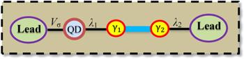
The considered system consists of a QD attached directly to the ferromagnetic lead and a Majorana wire, which is coupled to a metallic lead. The schematic illustration of this system is presented in figure 1. The studied system can be described by the following Hamiltonian(1)$\begin{eqnarray}H={H}_{C}+{H}_{{\mathtt{DM}}}+{H}_{t}.\end{eqnarray}$Here, H_C models the left and right contacts as reservoirs of noninteracting quasiparticles(2)$\begin{eqnarray}{H}_{C}=\displaystyle \sum _{k,\alpha =L,R,\sigma }{\varepsilon }_{k\alpha \sigma }{c}_{k\alpha \sigma }^{+}{c}_{k\alpha \sigma }^{},\end{eqnarray}$where ${c}_{k\alpha \sigma }^{+}$ is the creation operator for an electron with spin σ, momentum k and energy ϵ_kασ in the left or right lead. The second term H_DM accounts for the QD-Majorana wire system and it can be written as(3)$\begin{eqnarray}\begin{array}{rcl}{H}_{{\mathtt{DM}}} & = & \displaystyle \sum _{\sigma }{\varepsilon }_{d\sigma }{d}_{\sigma }^{+}{d}_{\sigma }+{{Un}}_{\sigma }{n}_{\bar{\sigma }}+{\mathtt{i}}{\varepsilon }_{M}{\gamma }_{1}^{}{\gamma }_{2}^{}\\ & & +\,{\lambda }_{1}({d}_{\sigma }^{}-{d}_{\sigma }^{+}){\gamma }_{1}^{},\end{array}\end{eqnarray}$where ${d}_{\sigma }^{+}({d}_{\sigma })$ is the creation (annihilation) operator for the dot with the energy ϵ_dσ, and U denotes the Coulomb interaction which is usually sufficiently large (U → ∞ ) for the forbidden of double occupancy. The Majorana quasiparticles are described by the operators γ₁₍₂₎. ϵ_M is the overlap between the wave functions of these two quasiparticles. The last term in equation (3) defines the coupling effect between the QD and Majorana wire, where λ₁ is the corresponding coupling element.

Figure 1.

New window|Download| PPT slide
Figure 1.Schematic representation of the system: A single level quantum dot (QD), coupled to a ferromagnetic (FM) leads with coupling strengths V_σ in the left part. λ₁ is the effective coupling strength between the QD and a topological superconducting wire (TSW) hosting Majorana bound states (MBSs) γ₁ and γ₂ at its ends, which is coupled to a metallic lead in the right part by the coupling strength λ₂.


The term H_t in equation (1) models for the tunneling processes between the QD-Majorana wire and the external leads, which is simply reads(4)$\begin{eqnarray}\begin{array}{rcl}{H}_{t} & = & \displaystyle \sum _{{kL},\sigma }({V}_{\sigma }{c}_{{kL}\sigma }^{+}{d}_{\sigma }^{}+{\mathtt{H}}.{\mathtt{C}}.)\\ & & +\,{\lambda }_{2}\displaystyle \sum _{{kR},\sigma }{\rm{i}}({c}_{{kR}\sigma }^{+}+{c}_{{kR}\sigma }^{}){\gamma }_{2}^{},\end{array}\end{eqnarray}$where λ₂ describes the coupling between the Majorana wire and the right lead. V_σ represents the tunneling matrix element between the left lead and the dot. The coupling to the left lead gives rise to the broadening of the dot, which can be described by ${{\rm{\Gamma }}}_{L}^{\sigma }=\pi {\sum }_{k\sigma }{\left|{V}_{\sigma }\right|}^{2}\delta (\varepsilon -{\varepsilon }_{{kL}\sigma })$ in the wide band limit. We can assume an up- and down-spin dependent coupling definition for the electrode in these considerations, namely ${{\rm{\Gamma }}}_{L}^{\uparrow \downarrow }=(1\pm p){{\rm{\Gamma }}}_{0}^{}$, in which p represents strength of the spin polarization. ${{\rm{\Gamma }}}_{0}^{}$ is the value at p = 0 and set to be the unit in our numerical results. The Majorana operators γ₁₍₂₎ can be represented by a fermionic creation f⁺ and annihilation operators f by defining ${\gamma }_{1}^{}=(f+{f}_{}^{+})/\sqrt{2}$ and ${\gamma }_{2}^{}=-{\mathtt{i}}(f-{f}_{}^{+})/\sqrt{2}$, which transforms the Hamiltonian H_DM as:(5)$\begin{eqnarray}\begin{array}{rcl}{H}_{{\rm{DM}}} & = & \displaystyle \sum _{\sigma }{\varepsilon }_{d\sigma }{d}_{\sigma }^{+}{d}_{\sigma }+{{Un}}_{\sigma }{n}_{\bar{\sigma }}+{\varepsilon }_{M}\left({f}_{M}^{+}{f}_{M}-\displaystyle \frac{1}{2}\right)\\ & & +\,\displaystyle \frac{{\lambda }_{1}^{}}{\sqrt{2}}({d}_{\sigma }^{}-{d}_{\sigma }^{+})({f}_{M}+{f}_{M}^{+}).\end{array}\end{eqnarray}$In this representation, the effective coupling between the Majorana wire and the right lead in equation (4) becomes:(6)$\begin{eqnarray}\begin{array}{rcl}{H}_{t} & = & \displaystyle \sum _{{kL},\sigma }({V}_{\sigma }{c}_{{kL}\sigma }^{+}{d}_{\sigma }^{}+{\mathtt{H}}.{\mathtt{C}}.)\\ & & +\,{\lambda }_{2}/\sqrt{2}\displaystyle \sum _{{kR},\sigma }({c}_{{kR}\sigma }^{+}+{c}_{{kR}\sigma })({f}_{M}-{f}_{M}^{+}).\end{array}\end{eqnarray}$We are interested in studying the influence of the Majorana wire on the physical properties of the QD mediated by the contact. To access the relevant physical quantities we employ the Green's function formalism, which allows us to obtain the spin-resolved DOS and the linear conductance of the system. According to the time-dependent evolution of the electron number in the left lead, the current through the left lead is defined as(7)$\begin{eqnarray}I=-e[\displaystyle \sum _{{kL}}{\dot{N}}_{{kL}}]=\displaystyle \frac{{\mathtt{i}}e}{h}\left\langle \displaystyle \sum _{{kL}}[{N}_{{kL}},H]\right\rangle .\end{eqnarray}$By introducing the relevant Keldysh non-equilibrium Green’s function method, we can further derive the Landauer current formula of this system [26](8)$\begin{eqnarray}I=\displaystyle \frac{2e}{h}\displaystyle \sum _{\sigma }\int ({f}_{L}(\varepsilon )-{f}_{R}(\varepsilon )){T}_{\sigma }(\varepsilon ){\rm{d}}\varepsilon ,\end{eqnarray}$where f_L(R)(ϵ) is the Fermi distribution function of the left (right) lead. T_σ(ϵ) is the transmission probability per spin given by ${T}_{\sigma }(\varepsilon )=\tfrac{{{\rm{\Gamma }}}_{L}^{\sigma }\cdot {\rm{\Lambda }}}{{{\rm{\Gamma }}}_{L}^{\sigma }+{\rm{\Lambda }}}\mathrm{Im}\ll {d}_{\sigma }^{},{d}_{\sigma }^{+}\gg $, where $\ll {d}_{\sigma }^{},{d}_{\sigma }^{+}\gg $ represents the retarded Green's function of the dot. Λ is the effective hybridization strength between the Majorana wire and the right lead defined by ${\sum }_{{kR}\sigma }\tfrac{{\lambda }_{2}^{2}}{2(\varepsilon +{\varepsilon }_{{kR}\sigma }^{})}\,={\sum }_{{kR}\sigma }\tfrac{{\lambda }_{2}^{2}}{2(\varepsilon -{\varepsilon }_{{kR}\sigma }^{})}=-{\mathtt{i}}{\rm{\Lambda }}$. We use the equation of motion (EOM) procedure to obtain the retarded Green's function of the dot [27](9)$\begin{eqnarray}\begin{array}{l}(\varepsilon +{\mathtt{i}}{0}^{+})\ll {d}_{\sigma },{d}_{\sigma }^{+}\gg \\ \quad =\,\left\langle \left\{\left.{d}_{\sigma },{d}_{\sigma }^{+}\right\}\right.\right\rangle +\ll \left[{d}_{\sigma },H\right],{d}_{\sigma }^{+}\gg ,\end{array}\end{eqnarray}$where H is the Hamiltonian given in equation (1) and 0⁺ is an infinitesimal number. In what follows, we will not write either the superscript i or the infinitesimal number 0⁺ for simplicity. For the dot, it is straightforward to write down the corresponding retarded Green's function $\ll {d}_{\sigma },{d}_{\sigma }^{+}\gg $ as(10)$\begin{eqnarray}\begin{array}{l}(\varepsilon -{\varepsilon }_{d\sigma }+{\mathtt{i}}{{\rm{\Gamma }}}_{L}^{\sigma })\ll {d}_{\sigma },{d}_{\sigma }^{+}\gg \\ \quad =1+U\ll {d}_{\sigma }{n}_{d\bar{\sigma }},{d}_{\sigma }^{+}\gg \\ \quad -\,{t}_{m1}(\ll {f}_{},{d}_{\sigma }^{+}\gg +\ll {f}_{}^{+},{d}_{\sigma }^{+}\gg ).\end{array}\end{eqnarray}$The term ${{\rm{\Gamma }}}_{L}^{\sigma }$ in equation (10) comes from the self-energy of the coupling between the lead and the dot and ${t}_{m1}={\lambda }_{1}/\sqrt{2}$ for simplicity. Now the new part in equation (10) for $\ll {f}_{}^{+},{d}_{\sigma }^{+}\gg (\ll f,{d}_{\sigma }^{+}\gg )$ can be simplified by their EOM procedure as follows:(11)$\begin{eqnarray}\begin{array}{l}(\varepsilon +{\varepsilon }_{M}+{\mathtt{i}}2{\rm{\Lambda }})\ll {f}_{}^{+},{d}_{\sigma }^{+}\gg \\ \quad =\,{t}_{m1}(\ll {d}_{\sigma }^{+},{d}_{\sigma }^{+}\gg -\ll {d}_{\sigma }^{},{d}_{\sigma }^{+}\gg )\\ \quad +{\mathtt{i}}2{\rm{\Lambda }}\ll {f}_{},{d}_{\sigma }^{+}\gg \\ \quad (\varepsilon -{\varepsilon }_{M}+{\mathtt{i}}2{\rm{\Lambda }})\ll {f}_{}^{},{d}_{\sigma }^{+}\gg ={t}_{m1}\\ \ \ \ \ \ \times \,(\ll {d}_{\sigma }^{+},{d}_{\sigma }^{+}\gg -\ll {d}_{\sigma }^{},{d}_{\sigma }^{+}\gg )\\ \quad +\,{\mathtt{i}}2{\rm{\Lambda }}\ll {f}_{}^{+},{d}_{\sigma }^{+}\gg .\end{array}\end{eqnarray}$Substituting the above equations into equation (10), we can derive the follow equation(12)$\begin{eqnarray}\begin{array}{l}(\varepsilon -{\varepsilon }_{d\sigma }+{\mathtt{i}}{{\rm{\Gamma }}}_{\sigma }^{L}-({\eta }_{1}(\varepsilon )+{\eta }_{2}(\varepsilon )){t}_{m1}^{2})\\ \quad \ll {d}_{\sigma },{d}_{\sigma }^{+}\gg =1+U\ll {d}_{\sigma }{n}_{d\bar{\sigma }},{d}_{\sigma }^{+}\gg \\ \quad -({\eta }_{1}(\varepsilon )+{\eta }_{2}(\varepsilon )){t}_{m1}^{2}\ll {d}_{\sigma }^{+},{d}_{\sigma }^{+}\gg ,\end{array}\end{eqnarray}$defining ${\eta }_{1}(\varepsilon )=\tfrac{(\varepsilon +{\varepsilon }_{M}+{\mathtt{i}}4{\rm{\Lambda }})}{(\varepsilon +{\varepsilon }_{M}+{\mathtt{i}}2{\rm{\Lambda }})(\varepsilon -{\varepsilon }_{M}+{\mathtt{i}}2{\rm{\Lambda }})+4{{\rm{\Lambda }}}^{2}}$, ${\eta }_{2}(\varepsilon )\,=\tfrac{(\varepsilon -{\varepsilon }_{M}+{\mathtt{i}}4{\rm{\Lambda }})}{(\varepsilon +{\varepsilon }_{M}+{\mathtt{i}}2{\rm{\Lambda }})(\varepsilon -{\varepsilon }_{M}+{\mathtt{i}}2{\rm{\Lambda }})+4{{\rm{\Lambda }}}^{2}}$ . Note that there are new higher parts $\ll {d}_{\sigma }{n}_{d\bar{\sigma }},{d}_{\sigma }^{+}\gg $ and $\ll {d}_{\sigma }^{+},{d}_{\sigma }^{+}\gg $ in equation (12), which can also be derived by their EOM procedure. Under the same approximation (leaving out the higher-correlation terms), we can get the closed Green's function of the above part, which can be written as follows:(13)$\begin{eqnarray}\begin{array}{l}(\varepsilon +{\varepsilon }_{d\sigma }+{\mathtt{i}}{{\rm{\Gamma }}}_{\sigma }^{L}-({\eta }_{1}(\varepsilon )+{\eta }_{2}(\varepsilon )){t}_{m1}^{2})\\ \quad \ll {d}_{\sigma }^{+},{d}_{\sigma }^{+}\gg =-U\ll {d}_{\sigma }^{+}{n}_{d\bar{\sigma }},{d}_{\sigma }^{+}\gg \\ \quad -\,({\eta }_{1}(\varepsilon )+{\eta }_{2}(\varepsilon )){t}_{m1}^{2}\ll {d}_{\sigma }^{},{d}_{\sigma }^{+}\gg ,\end{array}\end{eqnarray}$(14)$\begin{eqnarray}\begin{array}{l}(\varepsilon -{\varepsilon }_{d\sigma }+{\mathtt{i}}{{\rm{\Gamma }}}_{\sigma }^{L}-U-{t}_{m1}^{2}({\eta }_{1}(\varepsilon )+{\eta }_{2}(\varepsilon )))\\ \ll {d}_{\sigma }{n}_{d\bar{\sigma }},{d}_{\sigma }^{+}\gg =\left\langle {n}_{d\bar{\sigma }}\right\rangle -{t}_{m1}^{2}({\eta }_{1}(\varepsilon )\\ \quad +\,{\eta }_{2}(\varepsilon ))(\ll {d}_{\sigma }^{+}{n}_{d\bar{\sigma }},{d}_{\sigma }^{+}\gg )\\ \quad -\,{\eta }_{3}(\varepsilon )\ll {d}_{\sigma }^{},{d}_{\sigma }^{+}\gg \,,\end{array}\end{eqnarray}$(15)$\begin{eqnarray}\begin{array}{l}(\varepsilon +{\varepsilon }_{d\sigma }+{\mathtt{i}}{{\rm{\Gamma }}}_{\sigma }^{L}+U-{t}_{m1}^{2}({\eta }_{1}(\varepsilon )+{\eta }_{2}(\varepsilon )))\\ \quad \ll {d}_{\sigma }^{+}{n}_{d\bar{\sigma }},{d}_{\sigma }^{+}\gg =-{t}_{m1}^{2}({\eta }_{1}(\varepsilon )\\ \quad +\,{\eta }_{2}(\varepsilon ))(\ll {d}_{\sigma }^{}{n}_{d\bar{\sigma }},{d}_{\sigma }^{+}\gg )\\ \quad -\,{\eta }_{4}(\varepsilon )\ll {d}_{\sigma }^{+},{d}_{\sigma }^{+}\gg \,,\end{array}\end{eqnarray}$where ${\eta }_{3}(\varepsilon )={\sum }_{{kL}}\tfrac{{V}_{\sigma }^{2}f({\varepsilon }_{{kL}\bar{\sigma }})}{(\varepsilon -{\varepsilon }_{d\sigma }+{\varepsilon }_{d\bar{\sigma }}-{\varepsilon }_{{kL}\bar{\sigma }})}\,$ $\,+\tfrac{{t}_{m1}^{2}f({\varepsilon }_{M})}{(\varepsilon -{\varepsilon }_{d\sigma }+{\varepsilon }_{d\bar{\sigma }}+{\varepsilon }_{M})}\,$ $\,+\tfrac{{t}_{m1}^{2}f({\varepsilon }_{M})}{(\varepsilon +{\varepsilon }_{d\sigma }-{\varepsilon }_{d\bar{\sigma }}-{\varepsilon }_{M})}$ and ${\eta }_{4}(\varepsilon )={\sum }_{{kL}}\tfrac{{V}_{\sigma }^{2}f({\varepsilon }_{{kL}\bar{\sigma }})}{(\varepsilon +{\varepsilon }_{d\sigma }-{\varepsilon }_{d\bar{\sigma }}+{\varepsilon }_{{kL}\bar{\sigma }})}\,$ $\,+\tfrac{{t}_{m1}^{2}f({\varepsilon }_{M})}{(\varepsilon +{\varepsilon }_{d\sigma }-{\varepsilon }_{d\bar{\sigma }}-{\varepsilon }_{M})}\,$ $\,+\tfrac{{t}_{m1}^{2}f({\varepsilon }_{M})}{(\varepsilon +{\varepsilon }_{d\sigma }-{\varepsilon }_{d\bar{\sigma }}+{\varepsilon }_{M})}$. At this point, it is straightforward to obtain the retarded Green's functions of the dot. We will address the model either in the noninteracting (U = 0) or infinite interacting (U → ∞ ) cases. For U → ∞ , it is known to provide a fairly good description of Coulomb blockade phenomena. Within this approximation, the Green's functions of the two cases are as follows:(16)$\begin{eqnarray}\ll {d}_{\sigma },{d}_{\sigma }^{+}\gg =\displaystyle \frac{1}{{z}_{1}-\tfrac{{({\eta }_{1}(\varepsilon )+{\eta }_{2}(\varepsilon ))}^{2}{t}_{m1}^{4}}{{z}_{2}}}(U=0),\end{eqnarray}$(17)$\begin{eqnarray}\ll {d}_{\sigma },{d}_{\sigma }^{+}\gg =\displaystyle \frac{1-\left\langle {n}_{d\bar{\sigma }}\right\rangle }{{z}_{1}-\tfrac{{({\eta }_{1}(\varepsilon )+{\eta }_{2}(\varepsilon ))}^{2}{t}_{m1}^{4}}{{z}_{2}}}(U\to \infty ),\end{eqnarray}$where z₁ = ϵ − ϵ_dσ $\,+\,{\mathtt{i}}{{\rm{\Gamma }}}_{\sigma }^{L}-({\eta }_{1}(\varepsilon )\,$ $\,+\,{\eta }_{2}(\varepsilon )){t}_{m1}^{2}$ and z₂ = ϵ + ϵ_dσ $\,+\,{\mathtt{i}}{{\rm{\Gamma }}}_{\sigma }^{L}-({\eta }_{1}(\varepsilon )+{\eta }_{2}(\varepsilon )){t}_{m1}^{2}$. Throughout the next section, we will analyze the DOS and the linear conductance for different values of the energy ϵ_dσ, as well as the spin polarization strength p either in the noninteracting (U = 0) or the infinite interacting case (U → ∞ ). In this scenario the DOS can be written as DOS =$-(1/\pi ){\rm{Im}}\ll {d}_{\sigma },{d}_{\sigma }^{+}\gg $ for the QD.

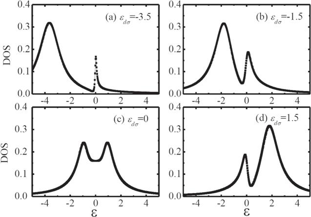
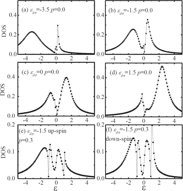
We first plot the DOS under different QD energy level ϵ_dσ in figure 2. The anti-resonance structure of the DOS forms around ϵ = 0 no matter how ϵ_dσ changes. The DOS shows bimodal symmetric structure when ϵ_dσ = 0. However it changes to bimodal asymmetric structure when ϵ_dσ ≠ 0, and one of the peaks moves to the lower energy level as the increase of ϵ_dσ. From the analytical process by solving the central Hamiltonian of the QD-CMBS part of the system [28], the position relationship between the double peak of the DOS will be simplified as the four energy eigenvalues as ${\varepsilon }_{\pm }^{2}={({E}_{+}(\varepsilon )\pm {E}_{-}(\varepsilon ))}^{2}$, where ${E}_{\pm }=\sqrt{{\left[\tfrac{1}{2}({\varepsilon }_{d\sigma }\pm {\varepsilon }_{M})\right]}^{2}+{t}_{m1}^{2}}$. When ϵ_dσ ≠ 0, the DOS has a dip structure, and two resonance structures will be symmetrically distributed on both sides. On the other hand, the DOS will exhibit an asymmetric structure if ϵ_dσ ≠ 0. The resonance position of DOS shifts, therefore an asymmetric resonance structure appears. The amplitude of the DOS decreases as the increase of ϵ_dσ, but the height of the peak does not drop. In the case of the special values of ϵ_M and t_m1, the self-adjoint behavior of Majorana fermions results in the characteristic of DOS, which is a remarkable signature of the presence of the Majorana zero mode leaking into the lead and the QD [29]. The Majorana operators are self-adjoint, namely ${\gamma }_{{\mathtt{i}}}={\gamma }_{{\mathtt{i}}}^{+}$ and thus they represent mixtures of particle and hole states, the interplay is manifested in the QD energy, which will destroy the symmetry property. When the QD energy level changes from ϵ_dσ = −3.5 to ϵ_dσ = 2, the interaction and the Majorana zero energy modes change, as shown in the asymmetrical-symmetrical-asymmetrical transition in the DOS. The DOS properties show different behaviors for these two different situations, based on which one can distinguish the whether there are MBSs in this system. It should be noted that we chose t_m1 and Λ without any changing values on the DOS and linear conductance. They don’t change much when we choose other t_m1 and Λ, which is enough to describe the Kondo–Majorana transport of the system.

Figure 2.

New window|Download| PPT slide
Figure 2.The DOS under different QD energy level ϵdσ, in the non-interaction case (U = 0), the other parameters are chosen as follows: ϵ_M = 0.05; p = 0; t_m1 = Λ = 0.5.


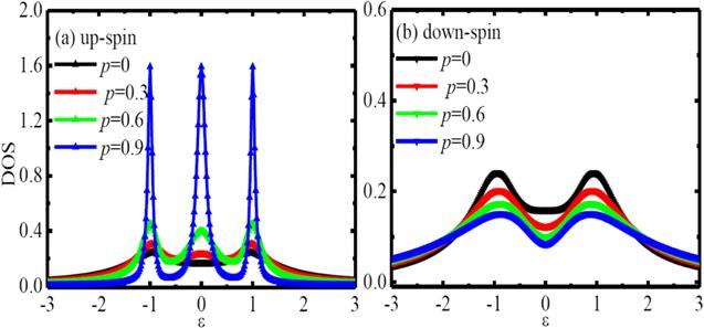
Next, we show the up- and down-spin DOS under different spin polarization strength in figure 3. In general, the up-spin DOS (figure 3(a)) increases with the increase of p. The up-spin DOS around zero energy increases and it exhibits the reversal process from an anti-resonance to resonance when p changes from p = 0 to p > 0.3. With the further increase of p, it presents a more obvious peak structure (p = 0.9). The peak structure also increases with the increase of the p. However, the down-spin DOS decreases with the increase of p as seen from figure 3(b). The down-spin DOS around zero energy also decreases with the increase of p. According to the definition of p, the effective coupling coefficient determines whether the DOS increases or decreases. For the up-spin DOS, ${{\rm{\Gamma }}}_{L}^{\uparrow }({{\rm{\Gamma }}}_{L}^{\downarrow })$ increases (decreases) with the increase of p, so the up-spin (down-spin) DOS increases with the increase of p. We can conclude that the up- (down-spin) resonance deceases with the increase of p. On the other hand, p does not only increase the up-spin DOS resonance but also shifts its peak position. This consideration clarifies why we have encountered the different up-and down-spin p dependence of the DOS. Note that the value of the down-spin DOS is smaller than that of the up-spin DOS, which is in accordance with the asymmetry hybridization between the up-spin and down-spins. Namely, ${{\rm{\Gamma }}}_{L}^{\uparrow }\geqslant {{\rm{\Gamma }}}_{L}^{\downarrow }$ determines that the up-spin (down-spin) DOS increases (decreases) with the increasing p. From the perspective of up- and down-spin value of the DOS in figure 3, we can also conclude that the up-spin is obviously beneficial to the total DOS. We hope to control the specific spin manipulation in the real experiment, which can be realized by controlling the up-spin state.

Figure 3.

New window|Download| PPT slide
Figure 3.The up- and down-spin DOS with different spin polarization strength p in the non-interaction case, ϵ_dσ = 0 and the other parameters are chosen the same as that in figure 2.


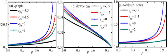
In order to clearly show the p and ϵ_dσ dependence on the DOS, we plot the up-and down-spin linear conductance as a function of the p under different ϵ_dσ in figure 4. The value of the up-spin linear conductance (figure 4(a)) is obviously larger than that of the down-spin linear conductance (figure 4(b)), which has the same properties as that shown in the DOS in figure 3. From this perspective, the up-spin conductance mainly contributes the total conductance passing through in the system. Specifically, the up-spin conductance shows an obvious increasing trend with the increase of p (p > 0.4). There is little difference between the value change of the conductance and the energy level of ϵ_dσ when p < 0.4. This is why the up-spin DOS (figure 3(a)) does not change much in the small p. We see an obvious conductivity increasing trend when the value of p is large (p > 0.4), which can also explain why the up-spin DOS show a transition from an anti-resonant structure to a resonant structure in figure 3(a) (p = 0.9). Correspondingly, we see that the down-spin conductance linearly decreases with the increase of p, which can be used to explain the sequential decrease in the DOS near zero energy level. When p is comparable large (p ≥ 0.6), the up-spin conductance increases fast when ϵ_dσ is small. Under the same spin polarization strength, we see that the conductance value is always at maximum when ϵ_dσ = 0 in contrasting to the case of ϵ_dσ = −3.5. For the fully polarized case with p = 1, the down-spin conductance will vanish in the present case in contrast to the up-spin. Through the further description of total linear conductance in figure 4(c), we see that the similarity between total linear conductance and the up-spin linear conductance. This is consistent with that shown in figure 3 where the up-spin contributes the main part of the DOS. The linear conductance does not change much when p < 0.4, and with the further increase of p. When p > 0.4, the increase of linear conductance under different is obvious. The conductance value at ϵ_dσ = 0 is the largest whether it is up-spin or down-spin. As the absolute value of increases, the linear conductance decreases, even we cannot see the linear conductance value when ϵ_dσ = −3.5. On the other hand, the conductance is mainly contributed by up-spin electrons in the large p region.

Figure 4.

New window|Download| PPT slide
Figure 4.The up- and down-spin linear conductance as a function of spin polarization strength under different QD energy level, the other parameters are chosen the same as that in figure 2.


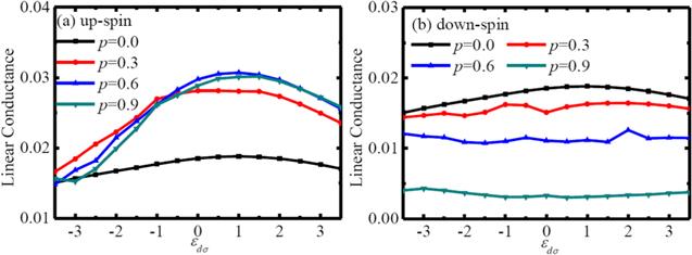
In this subsection we study the infinite interacting regime of the QD (U → ∞ ). In contrast to the previous subsection, we should emphasize that, the Green's function for spin σ determines on QD occupation n_σ given by $ \langle {n}_{\sigma } \rangle =-\tfrac{1}{\pi }{\int }_{-\infty }^{\infty }{\rm{Im}}\ll {d}_{\sigma }^{},{d}_{\sigma }^{+}\gg {\rm{d}}\omega $. We describe the properties of the linear conductance changing with ϵ_dσ of the system. From the specific up- and down-spin linear conductance in figure 5, the linear conductance under zero spin polarization is obviously different from the linear conductance under non-zero spin polarization with the change of ϵ_dσ. Although it increases with ϵ_dσ, the increase rate at non-zero is significantly greater than that at the zero case. And the linear conductance get the maximum near ϵ_dσ = 1, however, it tends to weaken with the further increase of ϵ_dσ correspondingly. With the introduction of the spin-polarization, the renormalized energy level of the QD causes an enhanced effect with the increase of p, but this enhancement will be restrained by the QD-MBS coupling. Also, it can be used to extract the important parameters of the Majorana's mutual interaction and its coupling to the lead. But the down-spin linear conductance does not change so much. Although it shows a weakening trend with the increase of p, it is smaller than the up-spin hybridization. With the change of ϵ_dσ, the dependence of p on the value of linear conductance is not obvious, namely, it shows a relatively equilibrium distribution when p changes from p = 0 to p = 0.9. Finally, the linear conductivity change rate is almost closing zero especially when p is relatively large (p = 0.9).

Figure 5.

New window|Download| PPT slide
Figure 5.The linear conductance as a function of ϵdσ under different spin polarization strength in the infinite interaction case (U → ∞ ), the other parameters are chosen as follows: ϵ_M = 0.05; t_m1 = Λ = 0.5.


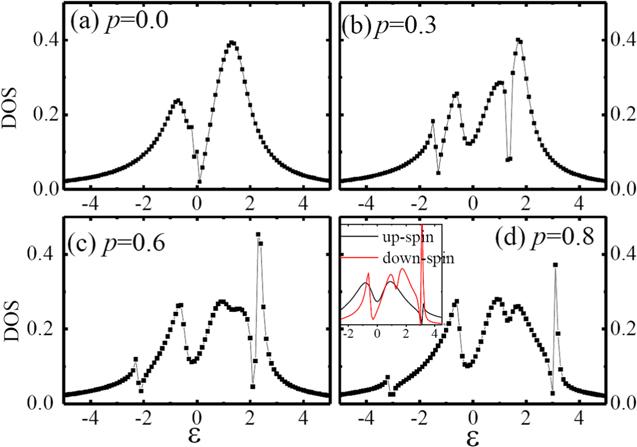
We plot the total DOS dependence on the spin polarization strength in figure 6. The notch structure of the DOS around ϵ_dσ = 0 will not change with the change of p. The Kondo resonance is located at energies coinciding with the renormalized energy of the QD. The renormalized calculation of the QD energy level causes its initial energy shifting because of the introduction of infinite interaction strength [30], where the real part of the denominator of η₃ and η₄ is found self-consistently from the relation ${\tilde{\varepsilon }}_{d\sigma }={\varepsilon }_{d\sigma }+\mathrm{Re}[{\eta }_{3}({\tilde{\varepsilon }}_{d\sigma },{\tilde{\varepsilon }}_{d\bar{\sigma }})+{\eta }_{4}({\tilde{\varepsilon }}_{d\sigma },{\tilde{\varepsilon }}_{d\bar{\sigma }})]$. Thus in the absence of spin polarization, the Kondo resonances is located on both sides of the Fermi level (${\tilde{\varepsilon }}_{d\uparrow }={\tilde{\varepsilon }}_{d\downarrow }$ ). From figure 6(a), we cannot see the DOS resonance splits when p = 0. However, the Kondo peak splits when p ≠ 0, giving rise to two sub-Kondo peaks. The splitting of the resonance peak structure is found at p = 0.3, 0.6, 0.8 because of the spin-dependent DOS in the leads. The hybridization is spin dependent, which is due to the splitting of the dot levels renormalized by the spin-dependent interacting self-energy (${\tilde{\varepsilon }}_{d\uparrow }\ne {\tilde{\varepsilon }}_{d\downarrow }$). In other words when the spin polarization is applied, the Kondo peak splits into two located peaks. We note that the Kondo resonances will appear at different positions without this self-consistency relation. The procedure simulates higher-order contributions of the dot-level on spin fluctuations. The introduction of p will not cause a change in the dip of the DOS, but it can cause the Kondo split on both sides of ϵ_dσ = 0. For the case of spin-polarized lead, the electron-lead interactions can induce a different occupation number (n_↑ ≠ n_↓) of the renormalized QD level which give rise to the exchange interaction in the ferromagnetic lead. Namely, the spin dependent hybridization causes the spin dependent occupancy number to decrease as p increases (n_↑ > n_↓), so the DOS will inevitably split with the increase of p. This weakening is more obvious for the down-spin DOS. We find that due to the energy split caused by the polarization, the down-spin DOS splits again compared with that in the up-spin DOS in the inset of figure 6(d). For comparing, we present the DOS at ϵ_dσ = − 3.5, − 1.5, 0, 1.5 for U → ∞ in figures 7(a)–(d). We see that a more obvious dip structure with the change of energy level ϵ_dσ . Such a peak transition still exists, which is the same as the peak transition as shown in figure 2. Therefore, we can conclude that such a relationship is sufficient to show the importance of the coupling relationship between Majorana and QDs. Unlike the case of U = 0, there is no bimodal symmetric structure when ϵ_dσ = 0. And this obviously comes from the renormalization of the QD energy level. As a comparison, we plot a specific DOS distribution in the case of ϵ_dσ = − 1.5 (figures 7(c) and (d)). Both the up-spin and down-spin DOS split with the change of p. Obviously, this split is consistent with that in figure 6. It should be noted that the introduction of the spin polarization leads to the renormalization distribution of the QD energy level, which leads to the difference in the up- and down-spin DOS. The down-spin peak is larger than the down-spin peak, however, they have the same split location. The contribution of ferromagnetic leads is to enhance the Kondo peak of the DOS.

Figure 6.

New window|Download| PPT slide
Figure 6.The total DOS under different spin polarization strength, the inset of (d) shows the explicit up- and down-spin DOS under large spin polarization strength (ϵ_dσ = 0, p = 0.8). The other parameters are chosen the same as that in figure 5.

Figure 7.

New window|Download| PPT slide
Figure 7.The total DOS under different QD energy level ϵ_dσ, in the infinite case (U → ∞ ), the other parameters are chosen the same as that in figure 5.


In summary, we have analyzed the spin-dependent Majorana–Kondo interplay of a QD-Majorana wire system. We have studied the behavior of the DOS and the linear conductance dependence on the dot-level and spin polarization strength of the lead. We demonstrated that the DOS resonance shifts with the change of energy level. The linear conductance show different characteristics for up- and down-spin directions characteristics under the spin polarized situation. Besides, the DOS shows a splitting behavior in the higher energy level with the increase of spin polarization strength. Our results reveal that the transport originates from the interplay between the Kondo correlations and the coupling to the topological Majorana wire. In this regard, the results presented in this paper may be applied to the spin-dependent hybrid Majorana-dot devices.

Reference View Option By original order
By published year
By cited within times
By Impact factor

[1]Alicea J 2012 Rep. Prog. Phys. 75076501
DOI:10.1088/0034-4885/75/7/076501 [Cited within: 1]

[2]Mourik V Zuo K Frolov S M Plissard S R Bakkers E P A M Kouwenhoven L P 2012 Science 336 1003
DOI:10.1126/science.1222360

[3]Deng M T Vaitiekenas S Hansen E B Danon J Leijnse M Flensberg K Nygard J Krogstrup P Marcus C M 2016 Science 354 1557
DOI:10.1126/science.aaf3961

[4]Wang J Zhang S-C 2017 Nat. Mater. 16 1062
DOI:10.1038/nmat5012 [Cited within: 1]

[5]Albrecht S M Higginbotham A P Madsen M Kuemmeth F Jespersen T S Nyga˙rd J Krogstrup,and P Marcus C M 2016 Nature 531 206
DOI:10.1038/nature17162 [Cited within: 1]

[6]Deng M-T Vaitiekénas S Prada E San-Jose P Nyga˙rd J Krogstrup P Aguado R Marcus C M 2018 Phys. Rev. B 98085125
DOI:10.1103/PhysRevB.98.085125

[7]Lee E J H Jiang X Aguado R Katsaros G Lieber C M Franceschi S De 2012 Phys. Rev. Lett. 109186802
DOI:10.1103/PhysRevLett.109.186802

[8]Lutchyn R M Bakkers E P A M Kouwenhoven L P Krogstrup P Marcus C M Oreg Y 2018 Nat. Rev. Mater. 3 52
DOI:10.1038/s41578-018-0003-1

[9]Das A Ronen Y Most Y Oreg Y Heiblum M Shtrikman H 2012 Nat. Phys. 8 887
DOI:10.1038/nphys2479

[10]Gül O et al. 2018 Nat. Nanotechnol. 13 192
DOI:10.1038/s41565-017-0032-8 [Cited within: 1]

[11]van der Wiel W G Franceschi S D Fujisawa T Elzerman J M Tarucha S Kouwenhoven L P 2000 Science 289 2105
DOI:10.1126/science.289.5487.2105 [Cited within: 1]

Goldhaber-Gordon D Shtrikman H Mahalu D Abusch-Magder D Meirav U Kastner M A 1998 Nature 391 156
DOI:10.1126/science.289.5487.2105 [Cited within: 1]

[12]Kondo J 1964 Prog. Theor. Phys. 32 37
DOI:10.1143/PTP.32.37 [Cited within: 1]

[13]Lee M Lim J S López R 2013 Phys. Rev. B 87241402
DOI:10.1103/PhysRevB.87.241402 [Cited within: 1]

[14]Liu D E Baranger H U 2011 Phys. Rev. B 84201308
DOI:10.1103/PhysRevB.84.201308 [Cited within: 1]

Cao Y Wang P Xiong G Gong M Li X-Q 2012 Phys. Rev. B 86115311
DOI:10.1103/PhysRevB.84.201308 [Cited within: 1]

[15]Liu C-X Sau J D Stanescu T D Sarma S Das 2017 Phys. Rev. B 96075161
DOI:10.1103/PhysRevB.96.075161 [Cited within: 1]

[16]Stenger J P T Woods B D Frolov S M Stanescu T D 2018 Phys. Rev. B 98 085407
DOI:10.1103/PhysRevB.98.085407

[17]Ruiz-Tijerina D A Vernek E Dias da Silva L G G V Egues J C 2015 Phys. Rev. B 91115435
DOI:10.1103/PhysRevB.91.115435 [Cited within: 1]

[18]Weymann I Wójcik K P 2017 Phys. Rev. B 95155427
DOI:10.1103/PhysRevB.95.155427 [Cited within: 2]

Yang F-B 2019 Physica E 109 164
DOI:10.1103/PhysRevB.95.155427 [Cited within: 2]

Yang F-B 2019 Commun. Theor. Phys. 71 1024
DOI:10.1103/PhysRevB.95.155427 [Cited within: 2]

[19]Golub A Kuzmenko I Avishai Y 2011 Phys. Rev. Lett. 107176802
DOI:10.1103/PhysRevLett.107.176802 [Cited within: 1]

Yang F-B 2018 Chin. Phys. Lett. 35077502
DOI:10.1103/PhysRevLett.107.176802 [Cited within: 1]

[20]Vernek E Penteado P H Seridonio A C Egues J C 2014 Phys. Rev. B 89165314
DOI:10.1103/PhysRevB.89.165314 [Cited within: 1]

[21]Weymann I Wójcik K P Majek P 1919 Phys. Rev. B 101235404
DOI:10.1103/PhysRevB.101.235404 [Cited within: 1]

[22]Misiorny M Weymann I Barnaś J 2011 Phys. Rev. Lett. 106126602
DOI:10.1103/PhysRevLett.106.126602 [Cited within: 1]

[23]Hauptmann J Paaske J Lindelof P 2008 Nat. Phys. 4 373
DOI:10.1038/nphys931

[24]Pasupathy A N Bialczak R C Martinek J Grose J E Donev L A K McEuen P L Ralph D C 2004 Science 306 86
DOI:10.1126/science.1102068 [Cited within: 1]

[25]Gaass M Hüttel A K Kang K Weymann I von Delft J Strunk C 2011 Phys. Rev. Lett. 107176808
DOI:10.1103/PhysRevLett.107.176808 [Cited within: 1]

[26]Yang F Cheng Y Liu F Chen X 2013 Appl. Phys. Lett. 103033513
DOI:10.1063/1.4815885 [Cited within: 1]

Yang F Cheng Y Liu F Chen X 2013 Appl. Phys. Lett. 102011911
DOI:10.1063/1.4815885 [Cited within: 1]

Yang F-B Huang R Cheng Y 2015 Physica B 464 77
DOI:10.1063/1.4815885 [Cited within: 1]

[27]Yang F-B 2019 Phys. Lett. A 383 1345
DOI:10.1016/j.physleta.2019.01.033 [Cited within: 1]

[28]Zeng Q-B Chen S Lü R 2016 Phys. Lett. A 380 951
DOI:10.1016/j.physleta.2015.12.026 [Cited within: 1]

[29]Ramos-Andrade J P Orellana P A Vernek E 2020 Phys. Rev. B 101115403
DOI:10.1103/PhysRevB.101.115403 [Cited within: 1]

[30]Martinek J Utsumi Y Imamura H Barnaś J Maekawa S König J Schön G 2003 Phys. Rev. Lett. 91127203
DOI:10.1103/PhysRevLett.91.127203 [Cited within: 1]