Wei Liu^,, Zhengxin Yan, Yixian WangCollege of Science, Xi’an University of Science and Technology, Xi’an 710054, China

Received:2020-06-5Revised:2020-10-13Accepted:2020-11-4Online:2021-01-07


Abstract
Using a Monte Carlo simulation and the single histogram reweighting technique, we study the critical behaviors and phase transitions of the Baxter–Wu (BW) model on a two-layer triangular lattice with Ising-type interlayer couplings. Via the finite-size analysis, we obtain the transition temperatures and critical exponents at repulsive and attractive interlayer couplings. The data for the repulsive interlayer coupling suggest continuous transitions, and the critical behaviors are the same as those of the 2D BW model, belonging to the four-state Potts universality class. The reduced energy cumulants and the histograms reveal that attractive coupling leads to weak first-order phase transitions. The pseudocritical exponents with the existence of the interlayer couplings indicate that the first-order transition is very close to the critical point of the 2D standard BW model.
Keywords： Baxter–Wu model;Monte Carlo simulation;critical behavior;weak first order phase transition


PDF (671KB)MetadataMetricsRelated articlesExportEndNote|Ris|BibtexFavorite
Cite this article
Wei Liu, Zhengxin Yan, Yixian Wang. Phase transitions of two spin-1/2 Baxter–Wu layers coupled with Ising-type interactions. Communications in Theoretical Physics, 2021, 73(1): 015602- doi:10.1088/1572-9494/abc7ac

1. Introduction

The study of spin models in statistical physics has great importance in many fields of science [1, 2]. Traditionally, the spin models can describe not only the magnetic properties of materials but also the surface adsorptions. Many researchers carried out mean-field approximations [3], renormalization-group method [4], exact solution [5], and Monte Carlo simulations [6, 7] in the frame of Ising models to study the surface phenomena of the bulk materials.

The adsorption and magnetic properties of multi-layered materials have been attracting lots of researchers in recent years due to their novel behaviors different from the bulk materials [8–10] and the potential technological applications such as high-density magnetic recording and magnetic sensors. Theoretically, the research for multilayer models could help us understand the crossover phenomena between two-dimension (2D) and three-dimension (3D) systems. Lots of studies concentrated on the magnetic properties of spin models built on bilayer lattices [11–13]. Recently, Žukovič et al [14, 15] have studied a bilayer Ising system consisting of two triangular planes with the antiferromagnetic (AF) coupling and the ferromagnetic (FM) one for the respective layers, which are coupled with the interlayer interaction by using Monte Carlo simulations. The heterostructure of frustrated and unfrustrated triangular-lattice layers results in critical behaviors close to the 2D 3-state Potts universality class instead of the 2D Ising class.

As for phase transitions in adsorbed monolayers, experimental studies have revealed that the critical behaviors belong to four-state Potts universality classes [16–18]. Consequently, D. W. Woods and H. P. Griffiths [19] proposed a magnetic model (Baxter–Wu (BW) model), which is defined in a two-dimensional triangular lattice. The spins are located in the vertices of the triangles and interact via a three spin interaction. R. J. Baxter and F. Y. Wu [20–22] solved the model at spin-1/2 exactly and find that it yields the same critical temperature of the Ising model on a square lattice and belongs to the four-state Potts universality class. Moreover, BW model as well as many other spin models on 2D triangular lattices [23–30], present relatively complicated transition behaviors. For example, the transitions of the finite size systems of the BW model display the discontinuities due to the low frequency large energy fluctuations [24]. The weak and pseudo-first-order phase transitions are also found in the Ashkin–Teller model [29, 30].

Recently, Jorge et al studied the 3D BW model [31], and found the distinct first order phase transition scaling behaviors. The additional degree of freedom causes the first-order phase transition. It would be interesting to study two layer BW models, which might present features not observed in the single-layer one. We studied a two-layer triangular lattice coupled with repulsive Ising couplings and found the corrections to the critical exponents caused by the interlayer interactions [32]. However, the first-order phase transition signals were not found in the systems. In this article, we concentrate on the two-layer BW model coupled with attractive interactions, and study behaviors of the phase transitions in the model. In section 2, we give the model and propose the simulation and data analyzing methods. The results are shown in section 3 with some discussion. Section 4 gives the conclusions of our work.

2. The model and the simulation methods

2.1. The model

The Hamiltonian for the BW model in the bilayer triangular lattice is$\begin{eqnarray*}E=-{J}_{A}\displaystyle \sum _{\langle {ijk}\rangle }{s}_{i}^{A}{s}_{j}^{A}{s}_{k}^{A}-{J}_{B}\displaystyle \sum _{\langle {ijk}\rangle }{s}_{i}^{B}{s}_{j}^{B}{s}_{k}^{B}+{J}_{{AB}}\displaystyle \sum _{i}{s}_{i}^{A}{s}_{i}^{B},\end{eqnarray*}$where, the spin variables are located at the vertices of the lattice within layer A or B and take the values ${s}_{i}^{A,B}=\pm 1$. ⟨ijk⟩ denotes the product of the three spins on the elementary triangle, and the sum is over all triads ⟨ijk⟩. The constants J_A and J_B are the three-body interaction within the layer A and B, and J_AB stands for the coupling constant between the layers A and B. We restrict to the case of J_A=J_B=1, and ∣J_AB∣≤1 in this work. The ground state of a single layer of the model is fourfold degenerate. We divide the bilayer triangular lattice into 3 interpenetrating sublattices as many researchers did in the single-layer lattice. The degenerate states are the single ferromagnetic state with all spins up and the three ferrimagnetic state with the spins on one sublattice up and the spins on the other two sublattices down.

2.2. Simulation methods

We apply the standard Metropolis Monte Carlo method to this model using N×N triangular lattice of individual planes with periodic boundary conditions. Typically 1×10⁶ MC steps per spin (MCS) were discarded and 2×10⁶ MCS were retained for the averages. We computed 4 times using different initial configurations to obtain the error bars. If error bars are not shown, they are always smaller than the size of the symbols. Measured thermodynamic quantities in our simulations are the magnetization per spin, specific heat, susceptibility, Binder cumulant and the reduced energy cumulant:(1)$\begin{eqnarray}m=\displaystyle \sum _{x}\langle | {m}_{x}| \rangle =\displaystyle \sum _{x}\left\langle \displaystyle \frac{1}{{N}_{\mathrm{tol}}}\left|\displaystyle \sum _{i\in (x)}{s}_{i}^{x}\right|\right\rangle ,\end{eqnarray}$(2)$\begin{eqnarray}{c}_{V}=\displaystyle \frac{\langle {E}^{2}\rangle -\langle E{\rangle }^{2}}{{N}_{\mathrm{tol}}{k}_{B}{T}^{2}},\end{eqnarray}$(3)$\begin{eqnarray}\chi =\displaystyle \frac{\langle {m}^{2}\rangle -\langle m{\rangle }^{2}}{{N}_{\mathrm{tol}}{k}_{B}T},\end{eqnarray}$(4)$\begin{eqnarray}{U}_{4}=1-\displaystyle \frac{\langle {m}^{4}\rangle }{3\langle {m}^{2}{\rangle }^{2}},\end{eqnarray}$(5)$\begin{eqnarray}{V}_{4}=1-\displaystyle \frac{\langle {E}^{4}\rangle }{3\langle {E}^{2}{\rangle }^{2}}.\end{eqnarray}$The subscript x is the symbol of the sublattices. N_tol equals N² if we just compute the quantites within a plane, while equals 2N² if we compute the quantities of the whole system. ⟨⋯⟩ denotes the thermal average taken over 2×10⁶ MCS. Lattice sizes from N=18 to N=120 are simulated, and the data are analyzed via the finite-size scaling.

2.3. Finite-size analysis

To obtain the critical exponents, we perform the finite-size scaling theory [33]. According to this theory, the thermodynamic properties obey the scaling forms, e.g.(6)$\begin{eqnarray}{c}_{V}\propto {N}^{\alpha /\nu },\end{eqnarray}$(7)$\begin{eqnarray}\langle m\rangle \propto {N}^{-\beta /\nu },\end{eqnarray}$(8)$\begin{eqnarray}\chi \propto {N}^{\gamma /\nu },\end{eqnarray}$where α, β, γ and ν are critical exponents which should obey the scaling relation at second order phase transitions. In addition, the Binder cumulants should approach to 2/3 below the critical temperature and to zero above the critical temperature. For a sufficiently large lattice size, the curves for the cumulants U₄ cross as a function of the temperature at a fixed point value K₀, and the location of the fixed point is the critical point.

However, the transition temperature obtained by the Binder cumulants is not very accurate. It is easier to deal with inverse temperature, so we define the quantity K=1/k_BT. To determine the transition temperature accurately, the location of peaks in thermodynamic derivatives defines an effective transition temperature K_c(N) to vary with system size, as(9)$\begin{eqnarray}{K}_{c}(N)={K}_{c}+\lambda {N}^{-1/\nu },\end{eqnarray}$where K_c is the inverse critical temperature at the thermodynamic limit and λ is a constant. Obviously, the value of ν is necessary to obtain the other critical exponents and the critical temperature at N∼∞. We use the relation of the maximum of the derivatives of $\mathrm{ln}m$ to obtain the exponent ν:(10)$\begin{eqnarray}{\left.\displaystyle \frac{\partial (\mathrm{ln}m)}{\partial K}\right|}_{\max }\propto {N}^{1/\nu }.\end{eqnarray}$

The reduced energy cumulant is used to analyze the order of the phase transitions [34]. The minimum of the reduced energy cumulant approaches the infinite lattice value according to the flowing equation.(11)$\begin{eqnarray}{V}_{4\min }={V}_{\inf }-{B}_{0}{N}^{-\alpha /\nu },\end{eqnarray}$where ${V}_{4\min }$, V_inf are the minimum values of the cumulants with finite size systems and with infinite systems respectively, and α/ν refers to the critical exponent. If V_inf equals to 2/3, the transition is of second order. If the value of V_inf is less than 2/3, the transition should be of the first order.

2.4. Reweighting technique

Performing a high-precision finite-size scaling analysis using standard MC techniques is very difficult, because locating the positions of the peaks of the thermodynamic quantities, which define the effective transition temperature T_c(L), requires multiple simulations in the vicinity of the peaks. This may take massive computer resources. The single histogram reweighting technique [35] extracts the information from Monte Carlo data at a single temperature, and enhances the potential resolution of Monte Carlo methods substantially. It is proved to be extremely precise for discussing both the first order and second-order phase transitions [35, 36].

First, we generate system configurations with a frequency proportional to $\exp (-{K}_{0}E)$ at K=K₀. The equilibrium probability distribution P(E, M) for some value of K can be written as(12)$\begin{eqnarray}P(E,M)=\displaystyle \frac{H(E,M)\exp ({\rm{\Delta }}{KE})}{{\displaystyle \sum }_{E,M}H(E,M)\exp ({\rm{\Delta }}{KE})},\end{eqnarray}$where ΔK=K−K₀ and M is the total magnetization. H(E, M) is the histogram of E and M kept during the simulation which gives an estimate for the equilibrium probability distribution. It becomes exact in the limit of an infinite-length run. Then the average of any function of E and M, ⟨g(E,M)⟩_K can be calculated form P(E, M) as a function of K(13)$\begin{eqnarray}\langle g(E,M){\rangle }_{K}=\displaystyle \sum _{E,M}g(E,M)P(E,M).\end{eqnarray}$Because our simulations do the finite length of the MC run, the single histogram equations (12) and (13) provide reliable results only for a narrow range of K values around K₀. The simulations are carried out at the lattice dependent effective inverse using 1×10⁷ MCS per site for sampling and 2×10⁶ for thermalization.

3. Results

3.1. The case of J_AB=1

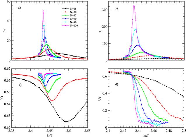
We studied the model with repulsive interlayer couplings in the article [32], and found that the phase transitions are continuous at our calculated strength of the interlayer couplings. In addition, if the coupling is weak enough, the behaviors of the transitions are very similar with the standard BW model which shows the pseudo-first-order phase transition [24], however, if the coupling is strong enough, the discontinuity of the transitions vanishes.

In order to compare to the attractive interlayer interactions, we present the case of repulsive interlayer interaction (J_AB=1) which shows the different transition behaviors from the standard BW model. As there exist the interlayer frustrations, it would be a good choice to compute magnetization and susceptibility within a specific layer. Typical data for the specific heat, the susceptibility, the Binder cumulants and the reduced cumulants are shown in figure 1. The specific heat and the susceptibility have peaks, and the peaks increase as the size of the system becomes larger. Besides, the cumulants cross at the fixpoint value K_0A=0.4115. All these suggest a second phase transition. We analyze our data for the reduced cumulants and obtain V_inf=0.6760±0.0005 which confirm the continuous phase transition. Then we calculate the quantities on different layers and under different initial conditions. Similar behaviors are found.

Figure 1.

New window|Download| PPT slide
Figure 1.The bulk properties as functions of the temperature at J_AB=1. (a) Specific heat on the whole systems, (b) susceptibility on a specific layer, (c) reduced energy cumulants on the whole systems and (d) Binder cumulants on the specific layer.


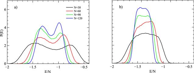
Schreiber et al's article [24] pointed out that the internal energy histograms of the single layer 2D BW model have double peaks, which suggest the pseudo-first-order phase transitions at the finite size systems. The reason for the phenomenon is the system is in a metastable states of coexistence of ferro- and ferri-magnetic order [24] as shown in figure 2(a). However, if the interlayer frustration is introduced, the repulsive interactions would break the states coexistence which make the histograms flat at the top. Figure 2(b) shows our simulation results for N=30, 60, 90 and 120. We believed that the energy distributions should reach the single peak form at N→∞.

Figure 2.

New window|Download| PPT slide
Figure 2.Non-normalized probability distributions of the internal energy obtained after 1×10⁷ sweeps at (a) J_AB=0 and (b) J_AB=1. The number on the vertical axis should be multiplied by 10 000.


Next, we applied the reweighting method to obtain the critical exponents and the critical temperatures, which can be estimated by considering the scaling behaviors according to equations (6)–(8). We obtained the exponents ν=0.662±0.009, α=0.657±0.011, β=0.079±0.015 and γ=1.165±0.011. The exponents imply that the bilayer BW model has the same universality class as the standard BW model, which belongs to the four-state Potts class. With ν in hand, we located K_c=0.411 67±0.000 05, which is slightly smaller than the value K_c=0.440 69 for the 2D BW model. Although the interlayer coupling brings frustration, it still leads to a higher transition temperature.

3.2. The case of attractive interlayer interactions

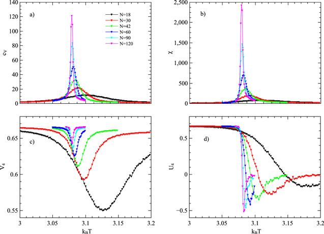
Then, we study the case of attractive interlayer interactions. The bulk properties for J_AB=−0.01, −0.1, −0.2, −0.5 and −1.0 are calculated. As there is no frustration, the thermodynamic quantities calculated in this section are based on the whole system. Typical data for the bulk quantities at J_AB=−1 are shown in figure 3. The specific heat and the susceptibility have peaks, and the peaks increase as the size of the system becomes larger as well. Different from the previous case, the Binder cumulants have negative minima, which usually appear on first-order phase transitions. However, when we check the finite size effect of specific heat: ${c}_{V\max }\sim {N}^{\alpha /\nu }$, we find α/ν<2 which should be 2 if the transition is of the first order. Similar behaviors are found at other interlayer couplings. Hence, alternative ways are needed to determine the order of the phase transitions at J_AB<0.

Figure 3.

New window|Download| PPT slide
Figure 3.The bulk properties as functions of the temperature at J_AB=−1. (a) Specific heat, (b) susceptibility (c) reduced energy cumulants and (d) Binder cumulant.


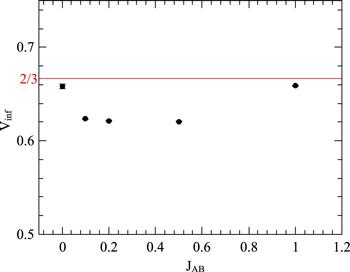
We compute the infinite lattice value of the reduced energy cumulants via the equation (11) and give the results in figure 4. All the values are less than 2/3 implying the first-order phase transition. We also observe that the value of V_inf at J_AB=−0.01 and −1.0 is closer to 2/3 than at J_AB equaling to other values. If the interlayer coupling is very weak, the behaviors would be very close to the standard BW model. The discontinuity would be very weak at thermodynamic limit. If the coupling becomes strong enough, the Ising-type coupling would domain the system. The discontinuity becomes weak as well. Only when the coupling constant is in the proper region we can observe the more obvious signal of a first-order phase transition. The further analyzing will be presented in the following via the histogram reweighting technique, which has been successfully applied to study the first-order phase transitions [36].

Figure 4.

New window|Download| PPT slide
Figure 4.The infinite lattice values of the reduced cumulants V_inf at different J_AB.


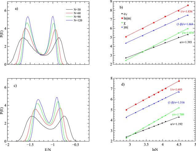
To identify the order of the phase transitions, we compute the energy histograms for N=30, 60, 90, and 120 at their effective transition temperature K_c(N) of the specific-heat peaks, which estimated from the standard MC simulations. The typical data at J_AB=−0.5 and −1.0 are shown in figures 5(a) and (c). The double peaks present in the graph which imply the first-order phase transitions. According to the theoretical predictions, the distribution peaks should have the same size [37], which is observed in our simulations. In addition, compared to figure 2(a), the depth of the valleys of the curves get larger as the size of the systems increase, which indicates that the histogram would reach a double-peak distribution at the thermodynamic limit. This is an obvious signal of the first-order phase transition. The histograms imply that the attractive couplings strengthen the possibility of ferro- and ferri-magnetic coexistence state, which results in the first-order phase transition.

Figure 5.

New window|Download| PPT slide
Figure 5.(a) and (c) Non-normalized probability distributions of the internal energy at J_AB=−0.5 and −1, respectively, obtained after 1×10⁷ sweeps. The number on the vertical axis should be multiplied by 10 000. (b) and (d) Size dependence of the maxima of $\mathrm{ln}m$, m, χ and c_V at J_AB=−0.5 and −1 respectively. The slopes yield corresponding critical exponents.


Applying the reweighting technique, we then obtain the pseudocritical behaviors and pseudo scalings. Figures 5(b) and (d) give the maximum of the corresponding quantities as a function of the lattice size. We plot the data of the log values and find excellent scaling behavior. The slopes for those quantities refer to the ‘pseudocritical exponents.’ We obtained ν=0.545, and 0.591 at J_AB=−0.5 and −1.0 respectively, which nearly equal to the value of the five-state Potts model [38]. We then compute four times with different initial conditions. Using the average values, we obtain the values of the exponents at different values of J_AB. The results are shown in table 1.


Table 1.
Table 1.The critical exponents.

	ν	α	γ	β
JAB=−0.1	0.551	0.753	1.022	0.092
JAB=−0.2	0.563	0.742	1.062	0.091
JAB=−0.5	0.556	0.758	1.021	0.092
JAB=−1.0	0.591	0.710	1.071	0.091

New window|CSV

We can check that the psedocritical exponents satisfy the scaling relation α+2β+γ≈2 while not the other relation dν−2β<γ. The values of the exponents are close to the values of the four-states Potts model. The good scaling behaviors indicate that the discontinuous is very weak, and the transition is very close to the critical point. Similar behavior has been observed for several models such as five-state Potts [37] and some frustrate Ising models [29, 30]. In these models, as well as our model, the correlation length is substantial. Hence one can observe explicit first-order scaling only if lattice size is much larger than the correlation length.

4. Conclusion

In summary, we use extensive Monte Carlo method to study BW model on the bilayer triangular lattices. The bulk properties are calculated to locate the effective transition temperatures and analyze the order of the transitions. Our data suggest that the system with repulsive interlayer coupling (J_AB=1) undergoes a second phase transition, while the attractive one (J_AB<0) undergoes a weak first-order phase transition. Via reweighting method and finite-size analyzing, we obtain the critical exponents and critical temperature for the repulsive inter-plane interaction. We find that the bilayer system has the same universality class as the single-layer BW model, which belongs to the four-state Potts universality class. For the attractive interlayer interactions, the reduced energy cumulants and the double peaks of the distributions of the energy confirm the first-order phase transition. Besides, we calculate the pseudocritical exponents and find that they are close to the four-Potts model’s exponents. We can get the conclusion that the phase transition for the system with the attractive interlayer coupling is the very weak first-order transition.

Acknowledgments

This work is supported by the National Science Foundation of China (Grant Nos. 11405127 and 11904282).

Reference View Option By original order
By published year
By cited within times
By Impact factor

[1]Christensen K Moloney N R 2005 Complexity and Criticality London Imperial College Press
[Cited within: 1]

[2]Yang B Li X-T Chen W Liu J Chen X-S 2016 Commun. Theor. Phys. 66 439
DOI:10.1088/0253-6102/66/4/439 [Cited within: 1]

[3]Mills D L 1971 Phys. Rev. B 3 3887
DOI:10.1103/PhysRevB.3.3887 [Cited within: 1]

[4]Burkhardt T W Eisenriegler E 1977 Phys. Rev. B 16 3213
DOI:10.1103/PhysRevB.16.3213 [Cited within: 1]

[5]Hu C-K Izmailian N S Oganesyan K B 1999 Phys. Rev. E 59 6489
DOI:10.1103/PhysRevE.59.6489 [Cited within: 1]

[6]Binder K Landau D P 1984 Phys. Rev. Lett. 52 318
DOI:10.1103/PhysRevLett.52.318 [Cited within: 1]

[7]Xiong G M Li X 2001 Commun. Theor. Phys. 35 114
DOI:10.1088/0253-6102/35/1/114 [Cited within: 1]

[8]Ju L et al. 2017 Science 358 907
DOI:10.1126/science.aam9175 [Cited within: 1]

[9]Shi W Liang R Xu S Wang Y Luo C Darwish M Smoukov S K 2015 J. Phys. Chem. C 119 13215
DOI:10.1021/acs.jpcc.5b01065

[10]Wu F Sarma S D 2019 Phys. Rev. B 99 220507(R)
DOI:10.1103/PhysRevB.99.220507 [Cited within: 1]

[11]Ferrenberg A M Landau D P 1991 J. Appl. Phys. 70 6215
DOI:10.1063/1.349999 [Cited within: 1]

[12]Szalowski K Balcerzak T 2012 Physica A 391 2197
DOI:10.1016/j.physa.2011.11.058

[13]Phu X P Ngo V T Diep H 2009 Surf. Sci. 603 109
DOI:10.1016/j.susc.2008.10.037 [Cited within: 1]

[14]Žukovic M Bobák A 2016 Phys. Lett. A 380 1087
DOI:10.1016/j.physleta.2016.01.016 [Cited within: 1]

[15]Žukovic M Tomita Y Kamiya Y 2017 Phys. Rev. E 96 012145
DOI:10.1103/PhysRevE.96.012145 [Cited within: 1]

[16]Domany E Schick M Walker J S Griffiths R B 1978 Phys. Rev. B 18 2209
DOI:10.1103/PhysRevB.18.2209 [Cited within: 1]

[17]Kim H K Chan M H W 1984 Phys. Rev. Lett. 53 170
DOI:10.1103/PhysRevLett.53.170

[18]Piercy P Pfnür H 1987 Phys. Rev. Lett. 59 1124
DOI:10.1103/PhysRevLett.59.1124 [Cited within: 1]

[19]Wood D W Griffiths H P 1972 J. Phys. C: Solid State Phys. 5 L253
DOI:10.1088/0022-3719/5/18/001 [Cited within: 1]

[20]Baxter R J Wu F Y 1973 Phys. Rev. Lett. 31 1294
DOI:10.1103/PhysRevLett.31.1294 [Cited within: 1]

[21]Baxter R J Wu F Y 1974 Aust. J. Phys. 27 357
DOI:10.1071/PH740357

[22]Baxter R J 1974 Aust. J. Phys. 27 369
DOI:10.1071/PH740369 [Cited within: 1]

[23]Novotny M A Landau D P 1981 Phys. Rev. B 24 1468
DOI:10.1103/PhysRevB.24.1468 [Cited within: 1]

[24]Schreiber N Adler J 2005 J. Phys. A: Math. Gen. 38 7253
DOI:10.1088/0305-4470/38/33/004 [Cited within: 4]

[25]Deng Y Guo W Heringa J R Blöte H W J Nienhuis B 2010 Nucl. Phys. B 827 406
DOI:10.1016/j.nuclphysb.2009.10.014

[26]Jorge L N Ferreira L S Leão S A Caparica A A 2016 Braz. J. Phys. 46 556
DOI:10.1007/s13538-016-0439-y

[27]Dias D A Xavier J C Plascak J A 2017 Phys. Rev. E 95 012103
DOI:10.1103/PhysRevE.95.012103

[28]Ding C Wang Y Zhang W Guo W 2013 Phys. Rev. E 88 042117
DOI:10.1103/PhysRevE.88.042117

[29]Jin S Sen A Sandvik A W 2012 Phys. Rev. Lett. 108 045702
DOI:10.1103/PhysRevLett.108.045702 [Cited within: 2]

[30]Liu R-M Zhuo W-Z Chen J Qin M-H Zeng M Lu X-B Gao X-S Liu J-M 2017 Phys. Rev. E 96 012103
DOI:10.1103/PhysRevE.96.012103 [Cited within: 3]

[31]Jorge L N Ferreira L S Caparica A A 2019 Phys. Rev. E 100 032141
DOI:10.1103/PhysRevE.100.032141 [Cited within: 1]

[32]Liu W Sun P Yan Z Wang Y 2020 Phys. Lett. A 384 126763
DOI:10.1016/j.physleta.2020.126763 [Cited within: 2]

[33]Landau D P Binder K 2009 A Guide to Monte Carlo Simulations in Statistical Physics3rd edn Cambridge Cambridge University Press
[Cited within: 1]

[34]Challa M S S Landau D P Binder K 1986 Phys. Rev. B 34 1841
DOI:10.1103/PhysRevB.34.1841 [Cited within: 1]

[35]Ferrenberg A M Swendsen R H 1988 Phys. Rev. Lett. 61 2635
DOI:10.1103/PhysRevLett.61.2635 [Cited within: 2]

[36]Ferrenberg A M Xu J Landau D P 2018 Phys. Rev. E 97 043301
DOI:10.1103/PhysRevE.97.043301 [Cited within: 2]

[37]Xu J Tsai S-H Landau D P Binder K 2019 Phys. Rev. E 99 023309
DOI:10.1103/PhysRevE.99.023309 [Cited within: 2]

[38]Peczak P Landau D P 1989 Phys. Rev. B 39 11932
DOI:10.1103/PhysRevB.39.11932 [Cited within: 1]