A. Rostami, K. Hajisharifi, H. Mehdian^,*, A. Hasanbeigi^*

Corresponding authors: * E-mail:k.hajishari@gmail.com

Received:2019-04-8Online:2019-10-9


Abstract
In this paper, the coupling instability of warm relativistic electron beam (WREB) propagating through the ion channel guiding is investigated in detail. Obtaining the equilibrium state of the system by considering the self-electric and azimuthal magnetic field, the fluid-Maxwell equations as well as linear perturbation theory are employed to derive the dispersion relation of the excited modes in the system. Numerical analysis of the obtained dispersion relation shows that the electromagnetic (EM) instability can be induced nearly the center of the beam through coupling between the fast electron plasma wave (FEPW), originated from the longitudinal oscillation of WREB, and fast forward electromagnetic wave (FFEW). In this sense, growing the perturbation amplitude occurs due to transport the kinetic energy of WREB to the EM wave at the specific frequency range, where the phase velocity of FEPW and FFEW is coincided. The results of the present investigation will greatly contribute to the understanding of the stability of the warm relativistic electron beam in laboratory experiments, such as in free electron laser experiments, where the ion-channel guiding is used to confine the electrons against the self-repulsive forces generated by the beam itself.
Keywords： coupling instability;warm relativistic electron beam;fluid-Maxwell equations;linear perturbation theory


PDF (860KB)MetadataMetricsRelated articlesExportEndNote|Ris|BibtexFavorite
Cite this article
A. Rostami, K. Hajisharifi, H. Mehdian, A. Hasanbeigi. Coupling Instability of a Warm Relativistic Electron Beam with Ion-Channel Guiding. [J], 2019, 71(10): 1236-1240 doi:10.1088/0253-6102/71/10/1236

1 Introduction

The physics of penetrating the relativistic electron beam (REB) into stationary background plasma is very important in various laboratories and applications, especially in ion channel production or in stable transmission of REB. The production of ion channel via various ways for many applications, such as development of the pulsed power laser, has become a topic of interesting researchers in the past years.^[1-2] There are different devices to produce ion channel which, one of these devices is injecting the relativistic electron beam into plasma environment. This relativistic electron beam can be cold or warm, which both methods have been used by previous researchers.^[3] As we know in the Budker condition by propagating the dense warm relativistic electron beam (WREB) into dilute plasma, the electrons of plasma environment will move away from the range of plasma radius and then ion channel will form. On the other hand, this beam can be focused by the space charge field of the ions, which is called ion focus regime (IFR). In this case the presence of ion channel makes the WREB able to stabile transmit in the plasma. But in this configuration, the beam electrons undergo betatron oscillations can couple with electromagnetic waves (EMW) in the channel. Therefore, to form an effective ion channel to guide the WREB stably transmitted in the space, the density of the WREB and ion channel must be well matched. Under the unstable conditions, the beam electrons can exchange its energy with electromagnetic wave (EMW) and dissipate through radiation. Obviously, in this system the self-fields of the beam electrons and the ion channel effects play an extremely important role in the entire physical process of the REB trajectory.^[4-6] Therefore, investigating these effects on the stability of beam plasma system in order to better understand the mechanism of the microwave radiation, the source of creating electromagnetic waves, the free electron laser using ion channel, the plasma wiggler x-ray, and other plasma radiation sources are important.^[7-12] Moreover, it can also be helpful for understanding the generations of the fast developing high power electromagnetic sources, such as the high power microwaves,^[13] millimeter waves,^[14] and sub-terahertz waves.^[15]

In this paper the stability propagation of REB passing through an ion channel is investigated using fluid model. Recalling the fluid Maxwell equation as well as employing the linear perturbation theory, the dispersion relation is derived to study the coupling instability excited in the considered system. Numerical analysis of the obtained dispersion relation shows that, the fast electron plasma wave interacts with the fast forward EM wave and can exchange their energy to growing the initial perturbation in a frequency domain that their phase velocities are the same. Results show that increment of ion channel density broadens the unstable frequency range, while decreases the maximum growth rate of the coupling instability. Moreover, increasing the temperature of the relativistic electron beam decreases the maximum growth rate of the instability, dramatically.

The paper is organized as follow: In Sec. 2, physical model of equilibrium state of system by considering the self-fields is presented. In Sec. 3, calling the Fluid-Maxwell equations, the linear perturbation theory is employed to obtain the dispersion relation of the perturbed system. At last, the numerical analysis of the obtained dispersion relation is used to investigate the coupling instability of WREB with ion-channel guiding in detail at Sec. 4.

2 Physical Model

Consider a relativistic electron beam (REB) with density $n_{e0}(r)$ propagating along a $\hat{Z}$ direction on the background ion channel with density $n_{i0}(r)$. This system can be obtained by passing the long REB with relatively high density (considering Budker condition) through an initial stationary plasma, through repulsion of background plasma electrons by the head of beam and assuming the massive background ions are fixed (unperturbed), and only takes to form a partial neutralization condition as

(1)$$ n_{i0}\left(r\right)=f\ n_{e0}(r)\,,$$
where $f=\text{const}=\text{fractional}$ neutralization. Moreover, it is assumed that the electrons have no mean motion in the azimuthal direction, that is,

(2)$$ {\beta{}}_{e\theta{}}(r)=\frac{v_{e0\theta{}}(r)}{c}=0\,. $$
For this considered system, the axial electron velocity is assumed to be independent of $r$, it means, $\beta_{bz}(r)=\beta_0=$const. As can be seen, in general, the system is infinite and uniform in the $\hat{Z}$ direction ${\partial{}{\psi{}}_0}/{\partial{}Z}=0$,where ${\psi{}}_0$ is unperturbed part of physical quantity in this system.Making use of Eqs. (1), (2) and generalizing the equilibrium force equation in the presence of self-field, including self-electric field and self-azimuthal magnetic field, the electron pressure $P_{e0}(r)$ at the equilibrium state can be found from Ref. ^[16]

(3)$$ \frac{1}{n_{e0}(r)}\frac{\partial{}}{\partial{}r}P_{e0}(r)=4\frac{\pi{}}{r^2}(1-f-{\beta{}}_0^2)\int_0^rr^{\prime}r^{\prime} n_{e0}(r^\prime)\,.$$
Choosing the isothermal state $P_{e0}(r)=n_{e0}(r)k_BT_e$ and considering the condition ${\beta{}}_0^2>1-f$, the density profile of the warm electron beam is obtained from this equation $n_{e0}(r)={n_{e0}(0)}/{{(1+({r^2}/{2\ r_b^2}))}^2}$, in which $r_b=\sqrt{{4{\lambda{}}_D^2}/({{\beta{}}_0^2-(1-f)})}$ where ${\lambda{}}_D=\sqrt{{{\epsilon{}}_0k_BT_e}/{n_0e^2}}$ is electron Debye length at $r=0$, $n_{i0}$ is the initial density of ions, and $n_{e0}$ stands for the initial density of WREB. The obtained electron density profile near the center of the beam, $r\ll r_b$, can be approximated with $n_{e0}(r)={n_{e0}(0)}/{{(1+({r^2}/{r_b^2})}})$. Note that, ${\beta{}}_0^2$ is assumed to be closed to $(1-f)$ and so $r_b\gg{}{\lambda{}}_D$.

3 The Electromagnetic Dispersion Relation of Beam

Considering the truly small time scale to ignore the ions motion, employing the linear perturbation theory the physical quantities can be written as

(4)$$\vec{\psi}=\vec{\psi}_0+\vec{\psi}_1\exp\left({i }\left(\omega{}t-kz\right)\right)\,,\quad {\psi{}}_1\ll{\psi{}}_0\,, $$
where $\vec{\psi}_1$ is the perturbed part of physical quantity $\vec{\psi}$. So, the current density and the velocity of the electron after perturbation can be expressed as follow

(5) $$ n_e=\frac{n_{e0}(0)}{(1+({r^2}/{r_b^2}))}+n_{e1}\exp({i}(\omega{}t-kz))\,, \\$$
(6)$$ \vec{v}=v_0\hat{k}\!+\!v_{r1}\exp({i}(\omega{}t\!-\!kz))\hat{r}\!+\!v_{z1}\exp({i}(\omega{}t\!-\!kz))\hat{k}\,. $$
Moreover, the perturbed parts of electric and magnetic fields by using the Maxwell equation have the form of

(7)$$ \vec{E}_1=E_{r1}\exp({i}(\omega{}t-kz))\hat{r}+E_{z1}\exp({i}(\omega{}t-kz))\hat{k}\,,\vec{B}_1=\frac{k}{\omega{}}E_{r1}\exp\left({i}\left(\omega{}t-kz\right)\right)\vec{\phi}\,.$$
The dynamic of the beam electrons follows the momentum transport equation as

(8)$$ n_0\frac{{d }\vec{p}}{d t}=-en_0(\vec{E_1}+\vec{v_0}\times\vec{B_1}+\vec{v_1}\times{}\vec{B_0})-\vec{\nabla}p_e\,,$$
where, $\vec{p}=\gamma{}m_0\vec{v}$ is the momentum of the beam electron and $m_0$ is the static electron mass. By substituting Eqs. (6) and (7) into Eq. (8), the perturbed velocity can be written as

(9)$$ v_{r1}=\frac{\eta/\gamma}{{\gamma{}}^2{\left(\omega{}-{kv}_0\right)}^2-{\omega{}}_B^2}\Big({i} \frac{{\gamma{}}^2{\left(\omega{}-{kv}_0\right)}^2}{\omega{}}E_{r1}-{\omega{}}_BE_{z1}-\frac{{i}k{\omega{}}_Bk_bT}{n_0e}n_1\Big), v_{z1}=\frac{\eta/\gamma}{{\gamma{}}^2{\left(\omega{}-{kv}_0\right)}^2-{\omega{}}_B^2}\Big(\frac{{\omega{}}_B\left(\omega{}-{kv}_0\right)}{\omega{}}E_{r1}+{i} \left(\omega{}-{kv}_0\right)E_{z1}-\frac{k\left(\omega{}-{kv}_0\right)k_bT}{n_0e}n_1\Big),$$
where $\eta{}={e}/{m_0}\ $is the charge-mass ratio, and ${\omega{}}_B={{\eta{}B}_0}/{\gamma{}}={{\omega{}}_{B0}}/{\gamma{}}$ is the electron cyclotron frequency. On the other hand, the linear forms of the perturbed current density components are

(10)$$ J_{r1}={\rho{}}_0v_{r1}\,,\quad J_{z1}={\rho{}}_0v_{z1}+{\rho{}}_1v_0\,,$$
in which ${\rho{}}_0={n_0e}/{(1+({r^2}/{r_b^2}))}$ is the charge density of the equilibrium state near the beam axis, and ${\rho{}}_1$ is the perturbed charge density.

Using the continuity equation $\vec{\nabla}\cdot \vec{J_1}=-({\partial{}{\rho{}}_1}/{\partial{}t})$, we can get

(11)$$ {\rho{}}_1=\frac{i(1-3({r^2}/{r_b^2})){\rho{}}_0}{r(1+({r^2}/{r_b^2}))(\omega{}-{kv}_0)}V_{r1}+\frac{{k\rho{}}_0}{(\omega{}-{kv}_0)}V_{z1}. $$
Now using the $\vec{\nabla}\cdot \vec{E}=({-e}/{{\epsilon{}}_0})n_1$,the perturbed electron density can be obtained as

(12)$$ n_1=-\frac{{\epsilon{}}_0}{er}E_{r1}+ik\frac{{\epsilon{}}_0}{e}E_{z1}. $$
Substituting Eqs. (9), (11), and (12) into Eq. (10) and using the tensor form of current density, $\vec{J}=\overleftrightarrow{\sigma}\cdot \vec{E}$ the component of dielectric tensor can be obtained from ${\epsilon{}}_r=1-({i\sigma{}}/{{\epsilon{}}_0\omega{}})$ as

$$ {\epsilon{}}_{11}=1-\frac{{\omega{}}_p^2}{({\gamma{}}^2{(\omega{}-kv_0)}^2-{\omega{}}_B^2)} \Big(\frac{{\gamma{}}^2{(\omega{}-kv_0)}^2}{{\omega{}}^2}+\frac{{\omega{}}_B\xi{}}{\omega{}}\Big),\\ {\epsilon{}}_{12}=\frac{I{\omega{}}_p^2}{({\gamma{}}^2{\left(\omega{}-kv_0\right)}^2-{\omega{}}_B^2)} \left(\frac{{\omega{}}_B}{\omega{}}\xi{}1\right), \\ {\epsilon{}}_{21}=\frac{-I{\omega{}}_p^2}{({\gamma{}}^2{\left(\omega{}-kv_0\right)}^2-{\omega{}}_B^2)} \Big(\frac{{\omega{}}_B\left(\omega{}-kv_0\right)}{{\omega{}}^2}-\frac{{\gamma{}}^2\left(\omega{}-kv_0\right) \left(1-3({r^2}/{r_b^2})\right)}{\omega{}}x-\frac{{\omega{}}_B\left(1-3({r^2}/{r_b^2})\right)}{\left(\omega{}-kv_0\right) \left(1+({r^2}/{r_b^2})\right)}x \xi{} \\ \hphantom{ {\epsilon{}}_{21}= }+\frac{kv_0{\omega{}}_B}{{\omega{}}^2}+\xi{}\Big), \\ {\epsilon{}}_{22}=1+\frac{{\omega{}}_p^2}{({\gamma{}}^2{\left(\omega{}-kv_0\right)}^2-{\omega{}}_B^2)} \Big(\frac{\left(\omega{}-kv_0\right)}{\omega{}}\xi{}1-\frac{\left(1-3({r^2}/{r_b^2})\right)}{\left(\omega{}-kv_0\right) \left(1+({r^2}/{r_b^2})\right)}x\xi{}1+\frac{kv_0}{\omega{}}\xi{}1\Big). \nonumber $$

Finally, by combining the dielectric tensor with the wave equation for an anisotropic medium yields

(13)$$ \nabla^2\vec{E_1}-\vec{\nabla}\left(\vec{\nabla}\cdot\vec{E_1}\right)+\frac{\omega^2}{c^2}\overleftrightarrow{\epsilon}\cdot \vec{E_1}=0\,, \\ $$
(14)$$ -k^2+\frac{{\omega{}}^2(1-\frac{(\frac{{\gamma{}}^2{(\omega{}-kv_0)}^2}{{\omega{}}^2}+\frac{\xi{}{\omega{}}_B}{\omega{}}){\omega{}}_p^2}{{\gamma{}}^2{(\omega{}-kv_0)}^2-{\omega{}}_B^2})}{c^2} \frac{1\omega{}{\omega{}}_B{\omega{}}_p^2}{c^2({\gamma{}}^2{(\omega{}-kv_0)}^2-{\omega{}}_B^2)} \\ -\frac{\omega{}^2(\xi{}-\frac{x{\gamma{}}^2(1-\frac{3r^2}{r_b^2})(\omega{}-kv_0)}{\omega{}}+\frac{kv_0{\omega{}}_B}{{\omega{}}^2}-\frac{x\xi{}(1-\frac{3r^2}{r_b^2}){\omega{}}_B}{(1+\frac{r^2}{r_b^2})(\omega{}-kv_0)}+\frac{(\omega{}-kv_0){\omega{}}_B}{{\omega{}}^2}){\omega{}}_p^2}{c^2({\gamma{}}^2{(\omega{}-kv_0)}^2-{\omega{}}_B^2)} \frac{{\omega{}}^2(1+\frac{(\frac{k\xi{}1v_0}{\omega{}}-\frac{x\xi{}1(1-\frac{3r^2}{r_b^2})}{(1+\frac{r^2}{r_b^2}) (\omega{}-kv_0)}+\frac{\xi{}1(\omega{}-kv_0)}{\omega{}}){\omega{}}_p^2}{{\gamma{}}^2{(\omega{}-kv_0)}^2-{\omega{}}_B^2})}{c^2} .$$
By setting the determinant of this matrix equal to zero, the normalized dispersion relation for this system can be obtained as

(15)$$ A+B \bar{\omega}+K \bar{\omega}^2+E \bar{\omega}^3+P \bar{\omega}^4+\mathit{\Upsilon} \bar{\omega}^6=0\,, $$
which the dispersion relation coefficients are

$$ \begin{eqnarray*} &&A=\bar{\xi}{\bar{\omega}_B}(-1+3\bar{r}^2)x {\xi}(-1+{\bar{\omega}_B}-(1+\bar{r}^2)(-1+\beta{}\mu{})\bar{\omega}_B)\\ &&B=\gamma (-(1+{\mathop{r}^{\_}}^2)(-1+\beta \mu )\xi {{\mathop{\omega }^{\_}}_B}^3+(-1+3{\mathop{r}^{\_}}^2)x\mathop{\xi }^{\_}(-(-1+{\mu }^2){{\mathop{\omega }^{\_}}_B}^2+\gamma (-1+\beta \mu )(1+(1+{\mathop{r}^{\_}}^2)(-1+\beta \mu ){\mathop{\omega }^{\_}}_B))),\\ &&K=(1+{\mathop{r}^{\_}}^2)\gamma (-1+\beta \mu )(-\mathop{\xi }^{\_}+\gamma {{\mathop{\omega }^{\_}}_B}^2)(\gamma (-1+\beta \mu )-(-1+{\mu }^2){{\mathop{\omega }^{\_}}_B}^2),\\ &&E={\gamma }^3{(-1+\beta \mu )}^2((-1+3{\mathop{r}^{\_}}^2)x(-1+{\mu }^2)\mathop{\xi }^{\_}+(1+{\mathop{r}^{\_}}^2)(-1+\beta \mu )\xi {\mathop{\omega }^{\_}}_B),\\ &&P=(-1-{\mathop{r}^{\_}}^2){\gamma }^3{(-1+\beta \mu )}^3({\gamma }^2(-1+\beta \mu )+(-1+{\mu }^2)\mathop{\xi }^{\_}-2\gamma (-1+{\mu }^2){{\mathop{\omega }^{\_}}_B}^2),\\ &&\mathit{\Upsilon}=-(1+{\mathop{r}^{\_}}^2){\gamma }^6{(-1+\beta \mu )}^5(-1+{\mu }^2).\end{eqnarray*}$$

In this relations, ${\omega }_p=\sqrt{{\eta \rho_0}/{{\gamma }_0{\epsilon }_0}}={{\omega }_{\mathrm{p0}}}/{\sqrt{{\gamma }_0}}$ is the plasma frequency of the electron beam, $\bar{\omega }=({\omega })/({{\omega }_{{{\rm p}0 }}})$ is the normalized frequency, $\bar{k}^{\_}={{k\ c}}/{{\omega }_{\mathrm{p0}}}$ is the normalized wave number, $\beta ={v_0}/{c}$ is the normalized velocity of the electron beam, $x={v_0}/{r\omega }={c\beta }/{r\omega }$ is the normalized velocity of light in vacuum,$\mathrm{\ }{\mathop{\omega }^{\_}}_B={{\omega }_B}/{{\omega }_{\mathrm{p0}}}$ is the normalized cyclotron frequency of the beam electrons, $\bar{r}={r}/{r_b}$ is the normalized radial distance from the beam axis, the refractive index is $\mu ={\rm Re }({\bar{k}}/{\bar{\omega }})$, and the imaginary part of refractive index is $X={\rm Im }({\bar{k}}/{\bar{\omega}})$. Moreover to find the present form of dispersion relation, we have defined $\bar{\xi }=1-{\lambda }^2k^2$ and $\xi ={{\lambda }^2k}/{r}$ as normalized constants.

4 Numerical Study of Dispersion Relation:Coupling Instabilities

In this system, the numerical method is employed to analyze the obtained dispersion relation Eq. (15). It is expected, from this investigation, coupling instability occurring due to the interaction between the electrostatic wave and the electromagnetic waves induced in passing WREB through initial ion channel, process observed in FEL and many laboratory systems can be extracted. In this numerical study we chose the WREB velocity, density and electron temperature \(\gamma_0=3\), \(n_{b0}=10^{18}\) \(m^{-3}\), and \(T=10^{6}\) \(^oK\), respectively, and also $r=10^{-5} {\rm m }$, where $r_b$ is considered to vary with partial neutralization and electron temperature.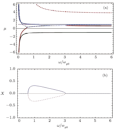

New window|Download| PPT slide
Fig. 1(Color online) (a) Real and (b) imaginary parts of the refractive index versus the normalized frequency at the $\bar{r}=0.02$ for the chosen parameters of system as $\gamma_0=3, n_{b0}=10^{18} {\rm m } ^{-3}$, and $T=10^{6}\,^{\rm o }{\rm K }$.



The real and imaginary parts of the refractive index versus normalized frequency, which is assumed to be real parameter, is illustrated in Figs. 1(a) and 1(b), respectively. As can be found from scrutiny of Fig. 1(a), six modes excited in the perturbed system are as follows: the red dash (solid) line is slow (fast) electron plasma wave originated from the longitudinal oscillations of WREB; the blue dash (solid) line is fast (slow) forward EM wave corresponding to the electromagnetic fluctuation of the applied perturbation; the black solid line is backward EM wave excited in the system as a transverse oscillation of the electromagnetic field propagating in the opposite direction of the beam motion; and finally the purple line is named beam mode shows the directional motion and transverse oscillation of beam electrons. The validity of these assertions can be checked by comparing the refractive index of the illustrated modes in Fig. 1(a) with the dispersion relation of the claimed modes related to each curves at the limiting values, such as $\omega\rightarrow\infty$. It is noted that in the mentioned limit when the frequency goes toward infinity, the phase velocity of the electromagnetic wave closes to the light velocity in the vacuum, $\mu=1$, while this condition is not evermore true for the electrostatic waves. To distinguish the modes shown in Fig. 1(a), the fast and slow labels are attributed to the similar waves through comparing their phase velocity at the fixed values of the wave frequency. Moreover, the backward and forward have been labeled to these waves according to the sign of phase velocities of them. The excited modes in the system are completely distinguished from each other until, the phase velocity of two waves matches together. In this sense, if one of the coupling waves is electrostatic and the other is electromagnetic, the coupling can be caused to the growing instability in the system through exchanging energy from the WREB to the electromagnetic fluctuation. As can be seen for the considered system under study, the phase velocity of the fast electron plasma wave (red solid line) and fast forward EM wave (blue dash line) is coincided to each other at the frequency range $0.6<\bar{\omega}<0.3$ . So in this range, transporting energy from WREB to the initial perturbation can be led to growing the coupling instability in the system. If the fast forward EM wave takes energy from fast electron plasma wave, the coupling instability occurs in the system (upper positive curve in Fig. 1) while in the contrary case, the damping of the perturbation is observed related to the lower negative curve of imaginary part of the refractive index.

New window|Download| PPT slide
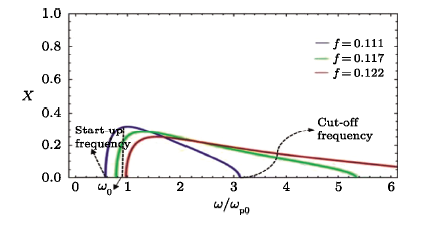
Fig. 2(Color online) The normalized growth rate of coupling instability versus normalized frequency for the three values of partial neutralization coefficient $f=0.111,0.117,0.122$, and the other chosen parameters as the same as Fig. 1.



In Fig. 2, the normalized growth rate of coupling instability versus normalized real frequency is depicted for the three values of partial neutralization coefficient $f=0.111,0.117$, and $0.122$. As seen from this figure, for the fixed value of WREB density $n_{b0}=10^{18} {\rm m}^{-3}$, increasing the ion channel density (increment of parameter $f$) the minimum unstable frequency (start-up frequency) and the maximum unstable frequency (cut-off frequency) increase dramatically. While, the increment of ion channel density decreases the maximum growth rate of the coupling instability occurs at a specific wave frequency $\omega_0$, called maximum frequency. It is observed from this figure that the maximum frequency increases by increasing the ion channel density.

New window|Download| PPT slide
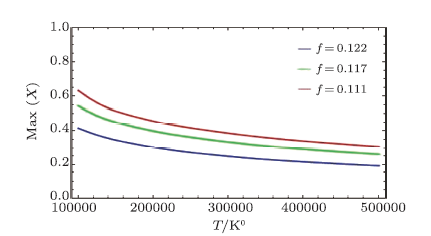
Fig. 3(Color online) The maximum growth rate of coupling instability versus the temperature of the WREB for three values of partial neutralization coefficient $f=0.111,0.117,0.122$, and the other chosen parameters as the same as Fig. 1.



We close this study by plotting the maximum growth rate of coupling instability against the temperature of the WREB in the range of \(T=10^{5}\) \(^oK\) to \(T=5\times 10^{5}\) \(\rm oK\) for three values of partial neutralization coefficient of system $f=0.111,0.117$, and $0.122$. As can be seen from this figure, for the fixed value of $f$, increasing the temperature of REB decreases the maximum growth rate of coupling instability. Moreover, at any temperature of the beam, it is shown that increasing the ion channel density decreases the maximum growth rate of instability, in agreement with the results of Fig. 3 illustrated for the specific temperature value \(T=10^{6}\) \(^oK\) .

Reference View Option By original order
By published year
By cited within times
By Impact factor

[1] R. Okamura, Y. Nakmura, N. Kawashima , Plasma Phys. 19(1977) 997.
[Cited within: 1]

[2] P. C. Jagher, F. W. Sluijter, H. J. Hopman , Phys. Rep. 167(1988) 177.
[Cited within: 1]

[3] G. J. Caporaso, F. Rainer, W. E. Martin , et al., Phys. Rev.Lett. 57(1986) 1591.
[Cited within: 1]

[4] A. Raghavi and H. Mehdian , Plasma Phys. Control. Fusion 53 2011) 105010.
[Cited within: 1]

[5] P. Rashed-Mohassel, A. Hasanbeigi, K. Hajisharifi , High Energy Density Physics 22 2017) 55.


[6] P. Rashed-Mohassel, A. Hasanbeigi, K. Hajisharifi , The European Physical Journal Plus 132 2017) 8.
[Cited within: 1]

[7] C. Joshi, T. Katsouleas, J. M. Dawson , et al., IEEE J. Quantum Electron. 23(1987) 1571.
[Cited within: 1]

[8] D. H. Whittum, A. M. Sessler, J. M. Dawson , Phys. Rev. Lett. 64(1990) 2511.


[9] R. L. Williams, C. E. Clayton, C. Joshi, T. C. Katsouleas , IEEE Trans. Plasma Sci. 21(1993) 156.


[10] W. Hoyer, A. Knorr, J. V. Moloney, E. M. Wright , Phys. Rev. Lett. 94(2005) 115004.


[11] J. S. T . Ng, et al., Phys.Rev. Lett. 87(2001) 244801.


[12] W. H. Bennett , Phys. Rev. 45(1934) 890.
[Cited within: 1]

[13] J. Wang , et al., Physics of Plasmas 16( 2009) 033108.
[Cited within: 1]

[14] X. Li , et al., IEEE Transactions on Electron Devices 60 ( 2013) 2931.
[Cited within: 1]

[15] J. Wang , et al., Scientific Reports 8 ( 2018) 6978.
[Cited within: 1]

[16] R. C. Davidson , Theory of Nonneutral Plasmas, Reading, Mass., Benjamin WA, Inc.( Frontiers in Physics. Volume 43), Vol. 43(1974) 213.
[Cited within: 1]