Meng-Yao Zhang, Zheng-Wen Long^,???, Chao-Yun Long^???College of Physics, Guizhou University, Guiyang 550025, China

Corresponding authors: ? ? E-mail:zwlong@gzu.edu.cn

Received:2018-12-11Online:2019-06-1

Fund supported:

Supported by the National Natural Science Foundation of China under Grant .11465006 Supported by the National Natural Science Foundation of China under Grant .11565009

PDF (849KB)MetadataMetricsRelated articlesExportEndNote|Ris|BibtexFavorite
Cite this article
Meng-Yao Zhang, Zheng-Wen Long, Chao-Yun Long. Solution of the Dipoles in Noncommutative Space with Minimal Length ^*. [J], 2019, 71(6): 640-646 doi:10.1088/0253-6102/71/6/640

1 Introduction

Most geometrical and topological effects can be realized in physics via studying the charged and neutral particles interact with the electric field and magnetic field. For instance, Aharonov-Bohm(AB) phase,^[1] Aharonov-Casher(AC) phase,^[2] and He-McKellar-Wilkens (HMW) phase.^[3-4] A well known quantum phase is Anandan phase proposed by Anandan,^[5] which describes a neutral particle moving in an external electromagnetic field with non-vanishing electric dipole moment and magnetic dipole moment. In 2001, Ericsson and Sjoqvist^[6] proposed the neutral particles interact with the non-zero electric field via a magnetic dipole moment can generate an analog of Landau quantization based on the AC interaction. Besides, motivated by the HMW interaction, Ribeiro et al.^[7] developed a quantization also similar to Landau quantization for neutral particles with a non-zero electric dipole moment.

After the concept of coordinate noncommutativity was first introduced by Snyder.^[8] The noncommutative theories are applied to the several areas of physics and have attracted large attention.^[9-11] The reason for the emergence of this attention was the discovery in string theory.^[12-13] Most results show that the noncommutative effect has influenced some physical phenomena, such as the AB effect,^[14-15] the AC effect,^[16-19] the HMW effect,^[20-21] quantum Hall effect,^[22-24] and Landau levels.^[25-27] On the other hand, the unification between the general theory of relativity and the quantum mechanics implies the existence of a minimal length $\Delta x_{\min}=\hbar\sqrt{\alpha }$. Further research shows that the minimal length can be introduced as an additional uncertainty in position measurement.^[28-31] So that the usual canonical commutation relation between position and momentum operators can be replaced by $ [ x_{i},p_{j} ]={\rm i}\hbar\delta _{ij}(1+\alpha p^{2})$,^[28-29] where $\alpha$ is a small positive parameter determined from a fundamental theory such as string theory.^[32-33] The modification of the uncertainty relation between position and momentum operators is usually termed generalized uncertainty principle (GUP) or the minimal length uncertainty principle.^[34]

Recently, considerable attention has been paid to the study of several physical problems in noncommutative coordinate space with minimal length uncertainty relation.^[35-39] In this work, we study a single neutral spin-half particle moves in an external electromagnetic field in noncommutative space with minimal length. The paper is organized as follows: In Sec. 2, we consider the Aharonov-Casher effect. In Sec. 3, He-McKellar-Wilkens effect is studied. Section 4 is our conclusions.

2 Aharonov-Casher Effect in Non-commutative Space with Minimal Length

In non-relativistic limit, considering the single neutral spin-half particle moving in an external electromagnetic field, and the particle possesses an electric dipole moment and a magnetic dipole moment, the Anandan Hamiltonian^[40] can be used to describe the system

(1) $H=-\frac{1}{2m}\Bigl[\bigtriangledown -i(\vec{\mu}\times\vec{E}) + i(\vec{d}\times \vec{B})\Bigr]^{2}-\frac{\mu}{2m} \bigtriangledown \cdot \vec{E}+\frac{d}{2m}\bigtriangledown \cdot \vec{B}\,,$
we adopt the system of natural unity were $\hbar=c=1$, and the terms of $O(\vec{E}^{2})$ and $O(\vec{B}^{2})$ are neglected, $\vec{\mu}$ is the magnetic dipole moment, $\vec{d}$ is the electric dipole moment, $\vec{E}$ is the electric field, and $\vec{B}$ is the magnetic field. In fact, the Hamiltonian consists two different physic effects, including Aharonov-Casher effect and He-McKellar-Wilkens effect. In which the particle interacts with electric field and magnetic field through the non-vanishing magnetic dipole moment and electric dipole moment.

Firstly, the Aharonov-Casher effect is considered, in which $d$ and $\vec{B}$ are absent, the electric field configuration can be expressed as $\vec{E}=({\rho }/{2})r\hat{e}_{\phi}$, where $\rho$ is the nonvanishing uniform charge density, and the Hamiltonian is given by

(2) $H=-\frac{1}{2m}[ \bigtriangledown -i\mu\vec{A}_{\rm AC}]^{2}-\frac{\mu}{2m}\bigtriangledown \cdot \vec{E}\,,$
the vector potential is defined as $\vec{A}_{\rm AC}=\vec{n}\times\vec{E}$, $\vec{n}$ is the unitary vector oriented in the dipole direction, and we choose the magnetic dipole to be parallel to the the $z$-direction, the associated field strength is $\vec{B}_{\rm AC}=\bigtriangledown \times \vec{A}_{\rm AC}$. It is worth noting that the magnetic field must be uniform for Aharonov-Casher system, torque vanishes on the dipole and electric field satisfies the conditions, $\partial _{t}\vec{E}=0$, $\bigtriangledown\times \vec{E}=0$, these conditions satisfy the restrictions of energy quantization.

In non-commutative spacetime the ordinary product is replaced by a star product of the form

(3) $(f\star g)(x)= \exp\Bigl(\frac{i}{2}\theta _{ij}\partial _{x^{i}}\partial _{x^{j}}\Bigr)f(x_{i})g(x_{j})\,,$
where $\theta _{ij}=\epsilon_{ij}\theta $ is the antisymmetric constant matrix, $\theta$ is the noncommutativity parameter, representing the antisymmetric tensor of dimension of (length)$^{2}$. The commutation relations between the spatial and momentum are given by

(4) $[\hat{x}_{i} ,\hat{x}_{j} ]= i\theta _{ij} ,\quad [ \hat{x}_{i}, \hat{p}_{j} ]= i\delta _{ij} , \\ [ \hat{p}_{i} ,\hat{p}_{j} ]=0 , \quad (i=j=1,2)\,.$
Considering the partical moves in the $x$-$y$ plane, in this case, the Schr$\ddot{o}$dinger equation in noncommutative space, which is written by

(5) $\Bigl \{ \frac{1}{2m} \Bigl [\Bigl(\hat{p}_{x}+\frac{\mu \rho }{2} \hat{y}\Bigr)^{2}+ \Bigr(\hat{p}_{y}-\frac{\mu \rho }{2}\hat{x} \Bigr)^{2}\Bigr ]-\frac{\mu \rho }{2m}\Bigr \}\psi =\epsilon\psi \,.$
It is possible to go back to the commutative space by replacing the noncommutative operators via Bopp shifts,^[41] so the relations between the noncommutative operators and commutative operators are obtained

(6) $\hat{x}=x-\frac{\theta }{2}p_{y}\,,\quad\hat{y}=y+\frac{\theta }{2}p_{x}\,,\quad\hat{p}_{x}=p_{x},\quad\hat{p}_{y}=p_{y}\,.$
By inserting Eq. (6) into Eq. (5), we rewrite the Schr$\ddot{o}$dinger equation as

(7) $\Bigl \{ \frac{1}{2M} (p_{x}^{2}+p_{y}^{2})+\frac{M\omega ^{2}}{8}(x^{2}+y^{2})-\frac{\omega }{2}L_{z}-k\Bigr \}\psi=\epsilon\psi\,,$
where

(8) $M{=}\frac{m}{(1{+}{\mu \rho \theta}/{4})^{2}}\,, \quad \omega {=}\frac{\mu \rho }{M(1{+}{\mu \rho \theta }/{4})}\,, \\ k{=}\frac{\omega }{2}\Bigl(1{+}\frac{\mu \rho \theta }{4}\Bigr)^{-1}\,.$
Now we introduce the minimal length formalism, the Heisenberg algebra is given by[28-29}

(9) $[ x_{i},p_{j} ] = i \delta_{ij} (1+\alpha p^{2})\,.$
This commutation relation leads to the standard Heisenberg uncertainty relation $\Delta x\Delta p\geq ({1}/{2})\delta _{ij}(1+\alpha(\Delta p)^{2} +\alpha \left \langle p \right \rangle^{2})$. A representation of $x_{i}$ and $p_{i}$ satisfies Eq. (9), may be taken as

(10) $x_{i} = i(1+\alpha p^{2})\frac{\partial }{\partial p_{i}}\,, \quad p_{i}=p_{i}\,.$
As well as writing the form of polar coordinates

(11) $p_{x} = p\cos \vartheta\,, \quad p_{y}=p \sin\vartheta\,, $
(12) $\frac{\partial }{\partial p_{x}}\! = \!\cos\vartheta \frac{\partial }{\partial p}-\frac{\sin\vartheta }{p}\frac{\partial }{\partial \vartheta}\,, \;\; \frac{\partial }{\partial p_{y}}\!=\!\sin\vartheta \frac{\partial }{\partial p} +\frac{\cos\vartheta }{p}\frac{\partial }{\partial \vartheta }\,.$
An auxiliary wave function is defined as $\psi (p,\vartheta )=e^{i\vartheta l }\varphi (p)$, then Eq. (7) becomes

(13) $\Bigl\{ (1+\alpha p^{2})^{2}\frac{\partial ^{2}}{\partial p^{2}}+ \Bigl[ \frac{1}{p} (1+\alpha p^{2} )^{2}+2\alpha p(1+\alpha p^{2})\Bigr] \frac{\partial }{\partial p}-\frac{l ^{2}}{p^{2}}(1+\alpha p^{2})^{2} -\frac{4}{M^{2}\omega ^{2}}p^{2} +\frac{4l }{M\omega }(1+\alpha p^{2}) +\frac{8}{M\omega ^{2}}(k+\epsilon) \Bigr\} \varphi (p)=0.$
Introducing a new variable $\zeta =({1}/{\sqrt{\alpha }})\arctan(\sqrt{\alpha }p)$,which maps the interval $\zeta \in (0, {\pi}/{2\sqrt{\alpha}})$,Eq. (13) is transformed into

(14) $\Bigl\{ \frac{\partial ^{2}}{\partial \zeta ^{2}} + \Bigl( \frac{\cos(\sqrt{\alpha }\zeta )}{\sin(\sqrt{\alpha }\zeta )} +\frac{\sin(\sqrt{\alpha }\zeta )}{\cos(\sqrt{\alpha }\zeta )}\Bigr)\sqrt{\alpha }\frac{\partial }{\partial \zeta } -\alpha l ^{2}\frac{\cos^{2}(\sqrt{\alpha }\zeta)}{\sin^{2}(\sqrt{\alpha }\zeta )} +\alpha Q\frac{\sin^{2}(\sqrt{\alpha }\zeta )}{\cos^{2}(\sqrt{\alpha }\zeta )}+\alpha \Omega \Bigr\}\varphi (\zeta )=0\,,$
where

(15) $Q = -l ^{2}-\frac{4}{M^{2}\omega ^{2}\alpha ^{2}}+\frac{4l }{M\omega \alpha}\,,$
(16) $\Omega =\frac{8(k+\epsilon)+4l \omega }{M\omega ^{2}\alpha }-2l ^{2}\,.$
Now, putting that $\varphi (\zeta ) = \cos^{\lambda }(\sqrt{\alpha }\zeta )F(\zeta )$,where $\lambda $ is an arbitrary constant, we arrive at

(17) $\Bigl\{ \frac{\partial ^{2}}{\partial \zeta ^{2}} + \Bigl ( \frac{\cos(\sqrt{\alpha }\zeta )}{\sin(\sqrt{\alpha }\zeta )} +(1-2\lambda )\frac{\sin(\sqrt{\alpha }\zeta)}{\cos(\sqrt{\alpha }\zeta )}\Bigr ) \sqrt{\alpha }\frac{\partial }{\partial \zeta } -\alpha l ^{2}\frac{\cos^{2}(\sqrt{\alpha }\zeta )}{\sin^{2}(\sqrt{\alpha }\zeta )} + \alpha [Q+\lambda (\lambda -1)-\lambda ]\frac{\sin^{2}(\sqrt{\alpha }\zeta )} {\cos^{2}(\sqrt{\alpha }\zeta )} +\alpha (\Omega-2\lambda )\Bigr\}F(\zeta )=0\,.$
The solution of Eq. (17) can be found by eliminating the term ${\sin^{2}(\sqrt{\alpha }\zeta )}/{\cos^{2}(\sqrt{\alpha }\zeta )}$,so we assume that

(18) $Q+\lambda (\lambda -1)-\lambda =0\,.$
Then the expression of $\lambda$ can be solved from above form

(19) $\lambda =1+\sqrt{1-Q}\,,\quad{\lambda }'=1-\sqrt{1-Q}\,.$
Since the term ${\lambda }'=1-\sqrt{1-Q}$ leads to a non-physically acceptable wave function, and then we simplify Eq. (17) into

(20) $\Bigl\{ \frac{\partial ^{2}}{\partial \zeta ^{2}} + \Bigl[ \frac{\cos(\sqrt{\alpha }\zeta )}{\sin(\sqrt{\alpha }\zeta )}+(1-2\lambda ) \frac{\sin(\sqrt{\alpha }\zeta)}{\cos(\sqrt{\alpha }\zeta )} \Bigr]\sqrt{\alpha } \frac{\partial }{\partial \zeta } -\alpha l ^{2}\frac{\cos^{2}(\sqrt{\alpha }\zeta )}{\sin^{2}(\sqrt{\alpha}\zeta )} + \alpha (\Omega-2\lambda)\Bigr\}F(\zeta )=0\,.$
Next we set $F(\zeta )=\sin^{|l |}(\sqrt{\alpha }\zeta )\phi (\zeta )$ as an auxiliary function, Eq. (20) can be written as

(21) $\Bigl\{ \frac{\partial ^{2}}{\partial \zeta ^{2}} +\Bigl[ (2|l| +1)\frac{\cos(\sqrt{\alpha }\zeta )}{\sin(\sqrt{\alpha }\zeta )}+(1-2\lambda ) \frac{\sin(\sqrt{\alpha }\zeta )}{\cos(\sqrt{\alpha }\zeta )} \Bigr]\sqrt{\alpha }\frac{\partial }{\partial \zeta } +\alpha (\Omega -2\lambda -2\lambda |l |) \Bigr\}\phi (\zeta )=0\,.$
In order to transform Eq. (21) into a class of known differential equations with a polynomial solution, we introduce another variable $z=2\sin^{2}(\sqrt{\alpha }\zeta )-1$, where $z\in (-1,1)$, and impose the following constraint

(22) $\frac{1}{4}(\Omega -2\lambda -2\lambda |l |)=n(n+|l |+\lambda )\,,$
where $n$ is a non-negative integer. So Eq. (21) becomes the form

(23) $\Bigl\{ (1-z^{2})\frac{\partial ^{2}}{\partial z^{2}}+[(|l |+1-\lambda )-(|l | +1+\lambda )z]\frac{\partial }{\partial z} +n(n+|l |+\lambda ) \Bigr\}\phi (z)=0,$
the solution of above equation can be reported by employing Jacobi polynomials as

(24) $\phi (z)=p_{n}^{(\lambda -1,|l |)}(z)\,.$
The eigenvalue equation of the system can be derived from Eq. (22)

(25) $\epsilon = \frac{1}{2}\Bigl ( n^{2}+n|l |+\frac{1}{2}l ^{2} \Bigr ) M\omega ^{2}\alpha -\frac{1}{2}l \omega -\frac{\omega }{2} \Bigl(1+\frac{\mu \rho \theta }{4} \Bigr)^{-1} + \frac{1}{2}\Bigl( n+\frac{1}{2}|l |+\frac{1}{2} \Bigr) \Bigl[ M\omega ^{2}\alpha + M\omega ^{2}\alpha \Bigl( 1+l ^{2} +\frac{4}{M^{2}\omega ^{2}\alpha ^{2}} -\frac{4l }{M\omega \alpha }\Bigr)^{1/2}\Bigr].$
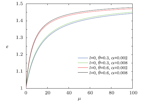
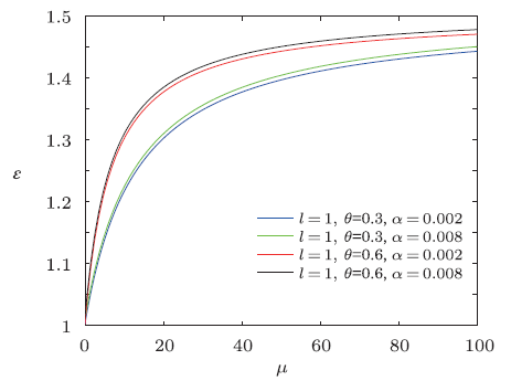
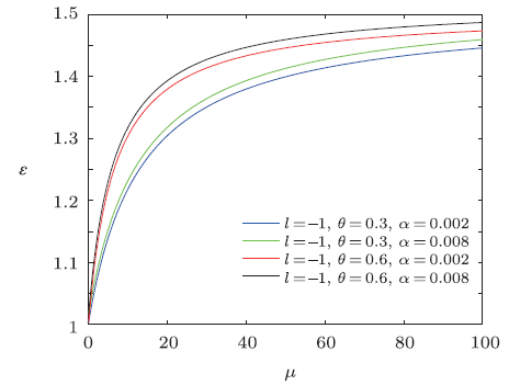
In order to visualize the influence of NC parameter and minimal length parameter on energy spectra, we decided to depict the energy spectra $\epsilon$ versus magnetic dipole moment $\mu$ for different values of the azimuthal quantum numbers by means of computer software, and the natural unit $n=M=\omega =\rho =1$ were employed. As shown in Figs. 1-3, each curve represents the profile of energy spectra $\epsilon$ versus magnetic dipole moment.

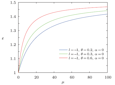
Fig.1

New window|Download| PPT slide
Fig.1The distribution of the energy spectra $\epsilon$ versus $\mu$ $(n=M=\omega =\rho =1)$.

Fig.2

New window|Download| PPT slide
Fig.2The distribution of the energy spectra $\epsilon$ versus $\mu$ $(n=M=\omega =\rho =1)$.

Fig.3

New window|Download| PPT slide
Fig.3The distribution of the energy spectra $\epsilon$ versus $\mu$ $(n=M=\omega =\rho =1)$.



From the results shown in Figs. 1-3, we see that the overall energy spectra increases monotonically with the increase of magnetic dipole moment, and the energy $\epsilon$ first rapidly increases then has a slow-growth. From the asymptotic behavior of the curve, it can be seen that the curves have similar linear behavior for the same NC parameter $\theta$. For a fixed value of magnetic dipole moment $\mu$, the energy spectrum increases when the minimal length parameter $\alpha$ grows for the same NC parameter $\theta$, and for the same minimal length parameter $\alpha$, the energy $\epsilon$ increases with the increase of NC parameter $\theta$.

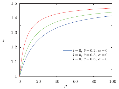
Now, we consider the special case of the ninimal length parameter is absent, that is $\alpha=0$, the eigenvalue equation degrades into

(26) $\epsilon_{\rm AC}=\Bigl(n+\frac{|l |-l +1}{2}-\frac{1}{2}\Bigr)\omega -\frac{\omega }{2}\Bigl(1+\frac{\mu \rho \theta }{4}\Bigr)^{-1}.$
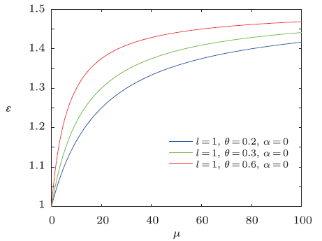
Obviously, it is strictly consistent with the result from Ref. ^[20]. The energy spectra $\epsilon$ versus magnetic dipole moment $\mu$ are plotted in Figs. 4-6, which show that overall energy spectra increase monotonically with the increases of the magnetic dipole moment. From the asymptotic behavior of the curve, we see that the energy $\epsilon$ rapidly increases at first for increasing $\mu$ then slowly grows for large $\mu$ values. The energy $\epsilon$ increases with the increase of NC parameter $\theta$ for a fixed value of $\mu$.

Fig.4

New window|Download| PPT slide
Fig.4The distribution of the energy spectra $\epsilon$ versus $\mu$ $(n=M=\omega =\rho =1)$.

Fig.5

New window|Download| PPT slide
Fig.5The distribution of the energy spectra $\epsilon$ versus $\mu$ $(n=M=\omega =\rho =1)$.

Fig.6

New window|Download| PPT slide
Fig.6The distribution of the energy spectra $\epsilon$ versus $\mu$ $(n=M=\omega =\rho =1)$.

3 He-McKellar-Wilkens Effect in Non-commutative Space with Minimal Length

In this section, the He-McKellar-Wilkens effect is studied, $\mu$ and $\vec{E}$ are absent in Eq. (1), the Hamiltonian of neutral particle moves in an external magnetic field can be written as

(27) $H=-\frac{1}{2m}[ \bigtriangledown +i d\vec{A}_{\rm HMW}]^{2}+\frac{d}{2m}\bigtriangledown \cdot \vec{B},$
where $\vec{A}_{\rm HMW}=\vec{n}\times \vec{B}$, and $\vec{n}$ is unitary and oriented in the dipole direction. Similarly, the magnetic field configuration can be expressed as $\vec{B}=({\rho _{m}}/{2})r\hat{e}_{r}$, where $\rho _{m}$ is the magnetic monopole charge density, the associated field strength can be defined as $\vec{B}_{\rm HMW}=\bigtriangledown \times \vec{A}_{\rm HMW}$.

In this case, He-McKellar-Wilkens magnetic field must be uniform, the torque may vanish on the dipole, the magnetic field satisfies the conditions, $\partial _{t}\vec{B}=0 $, and $\vec{B}$ must be smooth.

The Schr$\ddot{o}$dinger equation for the HMW system in NC space appears as

(28) $\Bigl\{ \frac{1}{2m} \Bigl[\Bigl(\hat{p}_{x}-\frac{d\rho _{m}}{2} \hat{y} \Bigr)^{2}+ \Bigl(\hat{p}_{y}+\frac{d\rho _{m}}{2}\hat{x} \Bigr)^{2}\Bigr]+\frac{d\rho _{m} }{2m}\Bigr\}\psi =\epsilon\psi.$
We change $\hat{x}_{i}$ by a Bopp shift in the Schr$\ddot{o}$dinger equation

(29) $\hat{x}=x-\frac{\theta }{2}p_{y}, \quad \hat{y}=y+\frac{\theta }{2}p_{x}.$
And the Eq. (28) takes the form

(30) $\Bigl\{ \frac{1}{2\tilde{M}} (p_{x}^{2}+p_{y}^{2}) +\frac{\tilde{M}\tilde{\omega}^{2}}{8}(x^{2}+y^{2}) +\frac{\tilde{\omega }}{2}L_{z}+\tilde{k}\Bigr\}\psi=\epsilon\psi\,,$
where

(31)$\tilde{M}=\frac{m}{(1+{d\rho_{m} \theta }/{4})^{2}}\,, \quad \tilde{\omega} =\frac{d\rho_{m}}{\tilde{M}(1+{d \rho_{m}\theta }/{4})}\,, \\ \tilde{k}=\frac{\tilde{\omega}}{2} \Bigl(1+\frac{d\rho_{m}\theta}{4}\Bigr)^{-1}\,. $
Now, we bring the problem into the momentum space

(32)$x_{i}=i(1+\alpha p^{2})\frac{\partial }{\partial p_{i}},\quad p_{i}=p_{i}.$
As well as writing the form of polar coordinates

(33) $p_{x}=p\cos\vartheta ,\quad p_{y}=p\sin \vartheta,$
(34) $\frac{\partial }{\partial p_{x}}=\cos\vartheta \frac{\partial } {\partial p}-\frac{\sin\vartheta }{p}\frac{\partial }{\partial \vartheta }\,, \\ \frac{\partial }{\partial p_{y}}=\sin\vartheta \frac{\partial }{\partial p} +\frac{\cos\vartheta }{p}\frac{\partial }{\partial \vartheta }\,.$
An auxiliary wave function is defined as $\psi (p,\vartheta )=e^{i\vartheta l }{\varphi }'(p)$, then Eq.(30) becomes

(35) $\Bigl\{ (1+\alpha p^{2})^{2}\frac{\partial ^{2}} {\partial p^{2}}+\Bigl [ \frac{1}{p} (1+\alpha p^{2} )^{2} +2\alpha p(1+\alpha p^{2})\Bigr ]\frac{\partial }{\partial p} -\frac{l ^{2}}{p^{2}}(1+\alpha p^{2})^{2} -\frac{4}{\tilde{M}^{2} \tilde{\omega}^{2}}p^{2}-\frac{4l }{\tilde{M}\tilde{\omega }}(1+\alpha p^{2}) +\frac{8}{\tilde{M}\tilde{\omega }^{2}}(\epsilon-\tilde{k}) \Bigr\}{\varphi }'(p)=0\,.$
By introducing a new variable $\tilde{\zeta} =({1}/{\sqrt{\alpha }}) \arctan(\sqrt{\alpha }p)$, which maps the interval $\tilde{\zeta }\in (0,{\pi }/{2\sqrt{\alpha }})$, Eq. (35) is transformed into

(36) $\Bigl\{ \frac{\partial ^{2}}{\partial \tilde{\zeta} ^{2}} + \Bigl( \frac{\cos(\sqrt{\alpha }\tilde{\zeta} )}{\sin(\sqrt{\alpha }\tilde{\zeta })} +\frac{\sin(\sqrt{\alpha }\tilde{\zeta })}{\cos(\sqrt{\alpha }\tilde{\zeta}) }\Bigr) \sqrt{\alpha }\frac{\partial }{\partial \tilde{\zeta}} -\alpha l ^{2}\frac{\cos^{2}(\sqrt{\alpha }\tilde{\zeta)}}{\sin^{2}(\sqrt{\alpha }\tilde{\zeta })} +\alpha \tilde{Q}\frac{\sin^{2}(\sqrt{\alpha }\tilde{\zeta })} {\cos^{2}(\sqrt{\alpha }\tilde{\zeta })}+\alpha \tilde{\Omega} \Bigr\}{\varphi }'(\tilde{\zeta }) = 0\,,$
where

(37) $\tilde{Q} = -l ^{2}-\frac{4}{\tilde{M}^{2}\tilde{\omega}^{2}{\alpha}^{2}}-\frac{4l }{\tilde{M}\tilde{\omega }\alpha }\,,$
(38) $\tilde{\Omega }=\frac{8(\epsilon-\tilde{k})-4l \tilde{\omega }}{\tilde{M}\tilde{\omega}^{2}\alpha }-2 l ^{2}\,.$
In this case, the energy spectra equation can be obtained by employing the same methods

(39) $\epsilon = \frac{1}{2}\Bigl({n'}^{2}+n'|l |+\frac{1}{2}l ^{2} \Bigr) \tilde{M}{\tilde\omega}^{2}\alpha +\frac{1}{2}l \tilde{\omega} +\frac{\tilde{\omega} }{2} \Bigl(1+\frac{d \rho_{m} \theta }{4}\Bigr)^{-1} +\frac{1}{2}\Bigl ( {n}'+\frac{1}{2}|l | +\frac{1}{2} \Bigr ) \\ \quad\times\Bigl [ \tilde{M}\tilde{\omega} ^{2}\alpha + \tilde{M}\tilde{\omega}^{2}\alpha \Bigl ( 1+l ^{2}+\frac{4}{\tilde{M}^{2}\tilde{\omega }^{2}\alpha ^{2}} +\frac{4l } {\tilde{M}\tilde{\omega }\alpha }\Bigr)^{1/2}\Bigr].$
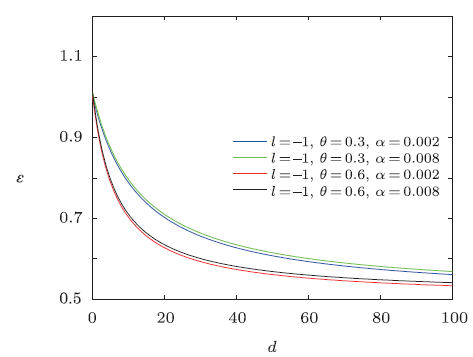
Similarly, it is difficult to analyse how the NC parameter and minimal length parameter affect the eigenenergy spectra, so we decide to depict energy spectra $\epsilon$ versus the electric dipole moments $d$ for different values of the azimuthal quantum number, and the natural unit ${n}'=\tilde{M}=\tilde{\omega }=\rho _{m}=1$ were employed. As shown in Figs. 7-9, each curve represents the profile of energy spectra versus electric dipole moment.

Fig.7

New window|Download| PPT slide
Fig.7The distribution of the energy spectra $\epsilon$ versus $d$ $({n}'=\tilde{M}=\tilde{\omega }=\rho _{m}=1)$.

Fig.8

New window|Download| PPT slide
Fig.8The distribution of the energy spectra $\epsilon$ versus $d$ $({n}'=\tilde{M}=\tilde{\omega }=\rho _{m}=1)$.

Fig.9

New window|Download| PPT slide
Fig.9The distribution of the energy spectra $\epsilon$ versus $d$ $({n}'=\tilde{M}=\tilde{\omega }=\rho _{m}=1)$.



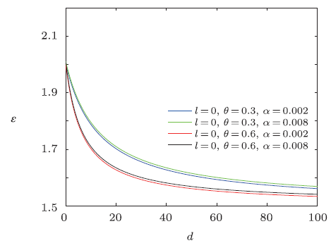
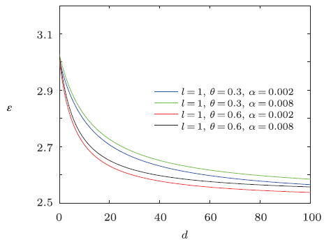
From the figures shown in Figs. 7-9, we see that the overall energy spectra decreases monotonically with the increase of electric dipole moment, and the energy $\epsilon$ first rapidly decreases then slowly decreases. From the asymptotic behavior of the curve, it can be seen that the curves have similar linear behavior for the same NC parameter. For a fixed value of electric dipole moment, the energy $\epsilon$ increases when the minimal length parameter grows for the same NC parameter $\theta$, and for the same minimal length parameter, the energy $\epsilon$ decreases with the increase of NC parameter $\theta$.

Subsequently, the special case of $\alpha=0$, that is for vanishing minimal length parameter, the eigenvalue equation degrades into

(40) $\epsilon_{\rm HMW} = \bigg({n}'+\frac{|l | + l +1}{2}+\frac{1}{2}\bigg)\tilde{\omega }+\frac{\tilde{\omega }}{2}\Bigl(1+\frac{d\rho _{m}\theta }{4}\Bigr)^{-1}.$
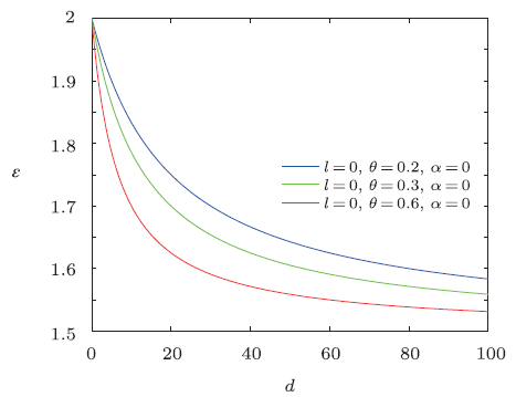
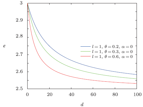
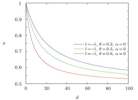
Obviously, it is strictly consistent with the result from Ref. ^[20]. The energy spectra $\epsilon$ versus $d$ are plotted in Figs. 10-12, which show that overall energy spectra decreases monotonically with the increase of electric dipole moment. From the asymptotic behavior of the curve, it can be seen that the energy spectra first rapidly decreases then has a slow-decrease. And the energy $\epsilon$ decreases with the increase of NC parameter $\theta$ for a fixed value of electric dipole moment.

Fig.10

New window|Download| PPT slide
Fig.10The distribution of the energy spectra $\epsilon$ versus $d$ $({n}'=\tilde{M}=\tilde{\omega }=\rho _{m}=1)$.

Fig.11

New window|Download| PPT slide
Fig.11The distribution of the energy spectra $\epsilon$ versus $d$ $({n}'=\tilde{M}=\tilde{\omega }=\rho _{m}=1)$.

Fig.12

New window|Download| PPT slide
Fig.12The distribution of the energy spectra $\epsilon$ versus $d$ $({n}'=\tilde{M}=\tilde{\omega }=\rho _{m}=1)$.

4 Conclusion

The non-relativistic quantum dynamic with a spin-half neutral particle, which possessing electric dipole moment and magnetic dipole moment in the presence of non-zero homogeneous electric and external magnetic fields was studied. We used the Hamiltonian found by Anandan to describe this system. The AC effect and HMW effect are investigated in the noncommutative coordinates space with minimal length. We transformed the Schr$\ddot{o}$dinger equation into a familiar form, the related energy spectra are obtained in terms of the Jacobi polynomials and we plotted corresponding numerical results. It shows that for AC system, the energy $\epsilon$ increases when the NC parameter and the minimal length parameter increase for the same azimuthal quantum number. The special case of the minimal length parameter $\alpha=0$ was discussed, and the corresponding numerical result was depicted respectively. It shows that the energy $\epsilon$ increases with the increase of NC parameter. And for HMW system, the energy $\epsilon$ increases with the increase of minimal length parameter but decreases with the growth of NC parameter. Similarly, when the minimal length parameter $\alpha=0$, the corresponding energy spectrum was depicted respectively. It shows that the energy $\epsilon$ decreases with the increase of NC parameter. Besides, the energy $\epsilon$ increases with the increase of the magnetic dipole moment for AC system but decreases with the increase of the electric dipole moment for HMW system.

The authors have declared that no competing interests exist.

Reference View Option By original order
By published year
By cited within times
By Impact factor

[1] Y. Aharonov and D. Bohm, Phys. Rev. 115(1959) 485.
[Cited within: 1]

[2] Y. Aharonov and A. Casher, Phys. Rev. Lett. 53(1984) 319.
[Cited within: 1]

[3] X. G. He and B. H. J. McKellar , Phys. Rev. A. 47 ( 1993) 3424.
[Cited within: 1]

[4] M. Wilkens , Phys. Rev. Lett. 72(1994) 5.
[Cited within: 1]

[5] J. Anandan , Phys. Rev. Lett. 85(2000) 1354.
[Cited within: 1]

[6] M. Ericsson and E. Sjoqvist , Phys. Rev. A 65( 2001) 013607.
[Cited within: 1]

[7] L. R. Ribeiro, C. Furtado, J. R. Nascimento , Phys. Lett. A. 348 ( 2006) 135.
[Cited within: 1]

[8] H. S. Snyder , Phys. Rev. 71(1947) 38.
[Cited within: 1]

[9] M. R . Douglas and N. A.Nekrasov, Rev. Mod. Phys. 73(2001) 977.
[Cited within: 1]

[10] J. W. Moffat , Phys. Lett. B 493 ( 2000) 142.


[11] A. Connes, M. R. Douglas, A. Schwarz , J. High Energy Phys. 02(1998) 003.
[Cited within: 1]

[12] N. Seiberg and E.Witten, J. High Energy Phys. 09(1999) 032.
[Cited within: 1]

[13] N. Seiberg, L. Susskind, N. Toumbas , J. High Energy Phys. 06(2000) 044.
[Cited within: 1]

[14] M. Chaichian, A. Demichev, P. Presnajder , et al., Phys. Lett. B 527 ( 2002) 149.
[Cited within: 1]

[15] K. Li and S. Dulat , Eur. Phys. J. C 46 ( 2006) 825.
[Cited within: 1]

[16] B. Mirza and M. Zarei , Eur. Phys. J. C 32 ( 2004) 583.
[Cited within: 1]

[17] S. Dulat and K. Li , Eur. Phys. J. C 54 ( 2008) 333.


[18] B. Mirza, R. Narimani, M. Zarei , Eur. Phys. J. C 48 ( 2006) 641.


[19] K. Li and J. Wang , Eur. Phys. J. C 50 ( 2007) 1007.
[Cited within: 1]

[20] L. R. Ribeiro, E. Passos, C. Furtado, J. R. Nascimento , Eur. Phys. J. C 56 ( 2008) 597.
[Cited within: 3]

[21] S. Dulat, K. Li, J. Wang, J. Phys . A: Math. Theor. 41(2008) 870.
[Cited within: 1]

[22] S. Dulat and K. Li , Eur. Phys. J. C 60 ( 2009) 163.
[Cited within: 1]

[23] O. F . Dayi and A. Jellal, J.Math. Phys. 43(2002) 4592.


[24] B. Basu and S. Ghosh , Phys. Lett. A 346 ( 2005) 133.
[Cited within: 1]

[25] P. A. Horvathy , Ann. Phys.(N.Y.) 299(2002) 128.
[Cited within: 1]

[26] P. A. Horvathy and M. S. Plyushchay , Nucl. Phys. B 714 ( 2005) 269.


[27] J. Gamboa, M. Loewe, F. Mendez, J. C. Rojas , Mod. Phys. Lett. A 16 ( 2001) 2075.
[Cited within: 1]

[28] A. Kempf , J. Math. Phys . 35(1994) 4483.
[Cited within: 2]

[29] A. Kempf, G. Mangano, R. B. Mann , Phys. Rev. D. 52 ( 1995) 1108.
[Cited within: 1]

[30] H. Hinrichsen and A.Kempf, J. Math. Phys. 37(1996) 2121.


[31] A. Kempf, J. Phys.A: Math. Gen. 30(1997) 2093.
[Cited within: 1]

[32] F. Brau and F. Buisseret , Phys. Rev. D. 74 ( 2006) 036002.
[Cited within: 1]

[33] H. Hassanabadi, S. Zarrinkamar, E. Maghsoodi , Phys. Lett. B. 718 ( 2012) 678.
[Cited within: 1]

[34] J. Y. Bang and M. S. Berger , Phys. Rev. D. 74 ( 2006) 125012.
[Cited within: 1]

[35] H. Hassanabadi, Z. Molaee, S. Zarrinkamar , Adv. High Energy Phys. 6(2014) 459345.
[Cited within: 1]

[36] A. Boumali and H. Hassanabadi , Z. Naturforsch. A. 70 ( 2015) 619.


[37] A. N. Ikot, H. P. Obong, H. Hassanabadi , Chin. Phys. Lett. 32(2015) 30201.


[38] S. R. Wu, Z. W. Long, C. Y. Long, B. Q. Wang, Y. Liu , Int. J. Mod. Phys. A. 32 ( 2017) 1750148.


[39] B. Q. Wang, Z. W. Long, C. Y. Long, S. R. Wu , Chin. Phys. B 27 ( 2018) 010301.
[Cited within: 1]

[40] E. Passos, L. R. Ribeiro, C. Furtado, J. R. Nascimento , Phys. Rev. A 76 ( 2007) 012113.
[Cited within: 1]

[41] T. Curtright, D. Fairlie, C. Zachos , Phys. Rev. D 58 ( 1998) 025002.
[Cited within: 1]