 ,1,*, A. Malik1, M. M. Rashidi2
Corresponding authors: * E-mail:laurel_lichen@yahoo.com
Received:2018-07-13Online:2019-04-1

Abstract
Keywords:
PDF (1710KB)MetadataMetricsRelated articlesExportEndNote|Ris|BibtexFavorite
Cite this article
S. Noreen, A. Malik, M. M. Rashidi. Peristaltic Flow of Shear Thinning Fluid via Temperature-Dependent Viscosity and Thermal Conductivity. [J], 2019, 71(4): 367-376 doi:10.1088/0253-6102/71/4/367
Nomenclature
 |
New window|CSV
1 Introduction
Latham[1] presented the pioneering work on peristaltic flows. A strong foundation was laid by him for development of peristalsis theoretically. He examined flow experimentally and analytically, in a two-dimensional channel. Peristalsis plays an important role in many industrial applications like blood pumps in heart and in sanitary fluid transport etc. This mechanism has various biological and biomedical systems, like motion of chyme in the gastrointestinal tract, circulation of blood in the blood vessels, transfer of spermatozoa in the ducts of the male reproductive tracts, transfer of ovum in the female fallopian tube, transportation of urine from kidneys to bladder and circulation of blood in the blood vessels. Shapiro it et al.[2] proposed the lubrication theory model in which a negligible effect of fluid inertia and wave number is taken into account. Since these works, many researchers have proposed mathematical model with wave trains, of wall generated flow due to difference in phase moving independently of the lower and upper walls. Recently, Rehman it et al.[3] have explained the peristaltic motion of Jeffrey fluid with effect of wall attributes. Convective boundary and inclined magnetic field effects on the peristaltic mechanism were studied by Noreen and Qasim.[4]Remarkable progress has been made by several authors during the previous few years in the development of flows for non Newtonian fluids. Heat transfer in peristalsis has also gained attention of researchers for last few decades. The process of transfer of heat may be used to get the details about the attributes of tissues. Currently, Rashidi it et al.[5-7] have done mentionable studies in investigation of flow of non-Newtonian fluids. Uddin it et al.[8] also made significant development in investigating the effect of free convection in the flow of real fluids. Bhatti it et al.[9] described the non-Newtonian fluid flow influenced by non- linear thermal radiation and MHD. Peristalsis has been the main subject of several recent research works. Undesirable tissues, such as cancer can be destroyed by heat. Inspired by above, Noreen and Qasim[10] presented a mathematical study for peristaltic motion of pseudoplastic fluid in a 2-D channel under certain approximations. Mention should be the name of Ramaesh and Devakar[11] for the progressive work in peristaltic flows in vertical channel. The non Newtonian fluid flow that was initiated by peristaltic waves in presence of chemical reaction was described by Noreen and Saleem.[12] Rundora and Makinde[13] synchronized the effects of suction/injection on unsteady non-Newtonian fluid flow in a channel filled with porous medium and convective boundary condition. Noreen[14] studied the induced magnetic field effect in peristaltic flow. A number of researchers are now busy in studying the peristalsis, particularly viscoelastic class of non-Newtonian fluids due to its wide range of applications in industry, engineering and medical science.
Fluid properties such as viscosity, density, thermal conductivity etc. are assumed constant for convenience in many studies. However variable fluid properties have real life applications, which include extrusion processes, fibre and wire coating, food-stuff processing, chemical processing equipment etc. Alvi it et al.[15] have examined the mixed convective peristaltic flow of Jeffrey nanofluid with variable viscosity, viscous dissipation and Joule heating effects. Latif it et al.[16] discussed the result of temperature-dependent variable properties on the third order peristaltic flow. Considering viscosity of the fluid as variable, studies[17-18] have also been reported.
Williamson fluid[19] is also a class of non-Newtonian fluids. Williamson fluid model is studied under various aspects in literature. Reddy it et al.[20] and Malik it et al.[21] described the Williamson fluid flow over a stretching sheet and stretching cylinder respectively. Few attempts in peristalsis are also available. Nadeem and Akram[22-23] peristaltic flow of Williamson fluid. Nadeem and Akbar[24] presented numerical solutions of Williamson fluid with radially varying MHD. In another article Vajravelu it et al.[25] presented peristaltic transport of a Williamson fluid with permeable walls. Variable properties effects on peristaltic transport of Williamson fluid are not studied before. The apparent viscosity varies gradually between $\mu _{\infty }$ as the shear rate tends to infinity and $\mu _{0}$ at zero shear rate. So, we try to fill this gap by studying the effects of variable thermal conductivity as well as variable viscosity on peristaltic transport of Williamson fluid with heat characteristics. The findings of the present study may be applicable in designing the peristaltic-pumps, transport phenomena in chemical engineering and energy systems, channel type solar energy collectors and heat exchangers.
Thermal analysis has been carried out for combined effects of variable conductivity and viscosity on peristaltic flow in the present article. The governing equations are introduced with boundary conditions. Double perturbation technique is employed to solve the system for closed form solution. Section 2 comprises of mathematical development and formulation of our problem. The zeroth and second order systems generated by using Perturbation technique are presented in Sec. 3. Finally the results are discussed in Sec. 4.
2 Problem Development and Formulation
We let that thermal conductivity $\bar{K} $ and viscosity $\bar{\mu}\ $of Williamson fluid vary linearly with temperature[16]where $K_{0}\ $is the thermal conductivity, $\mu _{0}\ $is fluid dynamic viscosity, $T_{w}$ is constant temperature and $\zeta $ and $\eta $ are constants.
2.1 Fluid Model
Constitutive equation of the Williamson fluid model with non constant viscosity is characterized bywith
with
The above model reduces to the Newtonian model $\Gamma =0$.
2.2Geometry of Problem
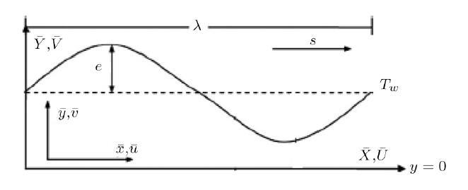
Let us consider a 2-D channel $(-H<\bar{Y}<\bar{H})\ $filled\ with Williamson fluid, of half width $c_{1}$. The walls of the channel are flexible and are subjected to constant temperature $T_{w}$. When the sinusoidal waves having small amplitude $e_{1}$ with constant speed $s\ $% propagate on the walls of the channel then the shape of the walls can be defined asHere $\bar{X} $ defines direction of wave propagation, $2\bar{c}_{1}\ $ defines the channel's width, $\lambda \ $is the wave length and $\bar{t}$ represents the time.
2.3 Basic Equations
The governing equations for Williamson fluid flow are:Defining a wave frame $(\bar{x},\bar{y})$ moving with velocity $s$ with respect to fixed frame $(\bar{X},\bar{Y})$ by the transformation:
yield
with
Now we define
After utilizing the dimensionless quantities and then solving the above equations.
Now introducing stream function $\psi (u={\partial \psi }/{\partial y} $, $v=-\delta {\partial \psi }/{\partial x})$, we arrive at
Here $W_{z}$, $Re$, $Ec$, $Pr $ and $ B_{k}$ represent the Weissenberg, Reynolds, Eckert, and Brinkman numbers respectively whereas $\delta $ is the wave number. Now applying the approximations of long wave and ignoring the terms of order $\delta $ and higher
Utilizing shear stress from above
Now eliminating pressure, we arrive at
2.4 Boundary Conditions
By aid of stream function $\psi $, boundary conditions are defined as:2.5 Volume Flow Rate
The volume flow rate in the fixed frame is given byIn the wave frame, the volume flow rate is defined as
The two rates of volume flow are related through
Over a period $T$, the time mean flow is defined as
In the wave frame, $F $ and $\theta $ the dimensionless time mean flow, are given by
where
3 Perturbation Solution
The closed form solution of the system of equations that comprises of non linear coupled differential equations is very challenging to find so, by using asymptotic analysis we produce the series solution. We take thermal conductivity parameter $\alpha $ and viscosity parameter $\epsilon$, of the same order of magnitude and asymptotically small, for the purpose of obtaining this. It may also be noticed that thermal conductivity parameter $\% \zeta $ and viscosity parameter $\eta $ are of same dimension $1/T$. So the heat equation can be written as:For finding the solution we apply the regular perturbation method. We expand $\psi $, $F $, and $P$ about fluid parameter $W_{z} $ and $\epsilon $
Now substituting the above expressions, we obtain the systems given below:
3.1 Order $(W_{z}^{o}, \epsilon ^{0 }) $ System
3.2 Order $(W_{z}^{1},\epsilon ^{0}) $ System
3.3 Order $(W_{z}^{0}, \epsilon ^{1})$ System
$$ \frac{\partial }{\partial y}\Big[ \frac{\partial \theta _{10}}{\partial y}\% +\theta _{00}\frac{\partial \theta _{00}}{\partial y}\Big] $$
3.4 Solution for System of Order $(W_{z}^{0}, \epsilon ^{0\ })$
3.5 Solution for System of Order $(W_{z}^{1}, \epsilon ^{0}) $
$$ \theta _{01} = \frac{1}{40h^{9}}\% [1Bk(-27F_{00}^{1}h^{5}-81F_{00}^{2}h^{6}-81F_{00}h^{7}+20F_{00}F_{01}h^{7}-27h^{8} +20F_{01}h^{8}+45F_{00}^{1}hy^{4}+115F_{00}^{2}h^{2}y^{4} \\ \hphantom{ \theta _{01} =} +115F_{00}h^{1}y^{4}-20F_{00}F_{01}h^{1}y^{4} +45h^{4}y^{4}-20F_{01}h^{4}y^{4}-18F_{00}^{1}y^{5}-54F_{00}^{2}hy^{5}-54F_{00}h^{2}y^{5}-18h^{1}y^{5})] \,. $$
3.6 Solution for System of Order $(W_{z}^{0}, \epsilon ^{1}) $
Using solution of above systems and
net results could be stated as:
The expression for pressure rise and heat transfer coefficient is
4 Discussion
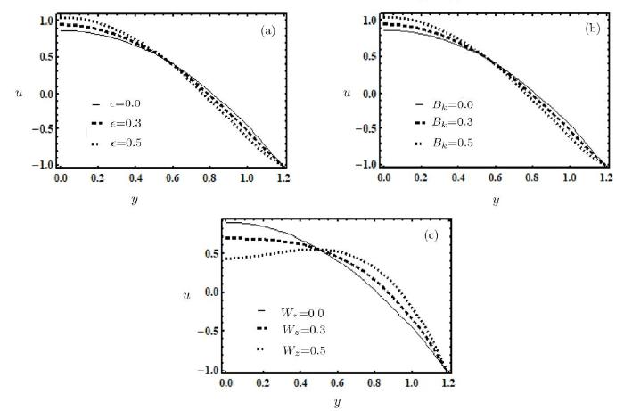
Influence of variable fluid properties on peristaltic flow of Williamson fluid has been discussed. The salient features of several physical parameters like velocity, pressure rise per wavelength, pressure gradient, heat transfer coefficient, temperature and streamlines have been described graphically. The reduced version of present study for fluid parameter $W_{z}$ and Brinkman number $Bk $ are in agreement with studies.[22-23]Figure 2 depicts the behavior of $\epsilon$, $ Bk$ and $W_{z} $ on velocity. At the center of the channel and near the channel walls, the behavior of the velocity is opposite. Figure 2(a) shows that at the center of the channel, the velocity increases as $\epsilon$ increases whereas the velocity decreases near the channel wall as $\epsilon$ increases. Brinkman number is the ratio between heat transported by molecular conduction and production of heat by viscous dissipation. Figure 2(b) shows that velocity increases at the center of the channel as $Bk$ increases while velocity decreases at the center of the channel as $Bk$ increases. Figure 2(c) represents decrease in velocity at the center of the channel as $W_{z}$ increases.
Fig. 1
 New window|Download| PPT slide
Fig. 1Flow configuration.
Fig. 2
 New window|Download| PPT slide
Fig. 2(a) Influence of $\epsilon $ on $u$ for $W_{z}=0.01$, $e=0.6$, $\theta =1.1$, $x=0.2$, and $Bk=0.9$. (b) Influence of $Bk$ on $u$ for $W_{z}=0.01$, $e=0.6$, $\theta =-1.5$, $\epsilon =0.1$, and $x=0.2$. (c) Influence of $W_{z}$ on $u$ for $Bk=2$, $e=0.6$, $\theta =-1.5$, $\epsilon =0.1$, and $x=0.2$.
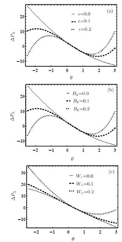
Figure 3 shows the behavior of $\epsilon$, $Bk $ and $W_{z} $ on pressure rise. The pumping against pressure rise is the most significant aspect of peristalsis. The retrograde pumping region is where $\Delta P_{\lambda }>0 $ and $\theta <0$. The fluid flow in this region is due to pressure gradient. The region where $\Delta P_{\lambda }>0 $ and $\theta >0 $ is known as peristaltic pumping region. The fluid that is moved in forward direction and the peristalsis of walls in this region overcomes the resistance of pressure gradient. The free pumping zone is where $\Delta P_{\lambda }=0 $ and the volume flow rate $\theta $ is known as free pumping flux. In the region where $\Delta P_{\lambda }<0 $ and $\theta >0 $ is the copumping region. It is observed that increase in $\epsilon $ means increase in the thermal conductivity/variable viscosity. Figure 3(a) shows that the pressure decreases as $\epsilon $ increases in the retrograde region while in the copumping region it behaves oppositely. The effect on $% \Delta P_{\lambda } $ for $Bk $ is the same as that of $\epsilon $ in Fig. 3(b). It is noticed that $\Delta P_{\lambda }$ in Fig. 3(c), increases as $W_{z} $ increases in the retrograde region whereas its behavior is opposite in copumping region. It is noticed that in the peristaltic pumping region, $% \Delta P_{\lambda } $ shows no deviation under all type of variations.
Fig. 3
 New window|Download| PPT slide
Fig. 3(a) Influence of $\epsilon $ on $\Delta P_{\lambda }$ for $Bk=0.8$, $e=0.5$, and $W_{z}=0.02$. (b) Influence of $Bk$ on $\Delta P_{\lambda }$ for $\epsilon =0.8$, $e=0.5$, and $W_{z}=0.02$. (c) Influence of $W_{z}$ on $\Delta P_{\lambda }$ for $Bk=0.8$, $e=0.5$, and $\epsilon =0.02$.
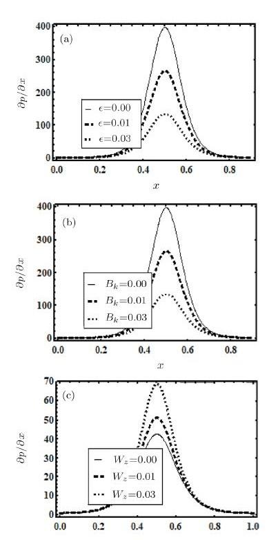
Figure 4 illustrates the behavior of $\epsilon$, $Bk$ and $W_{z} $ on pressure gradient. It is observed that at the wider part of the channel when $x=0$, the pressure gradient is very small. This can be justified physically because without the assistance of huge pressure gradient, the fluid can pass easily. Whereas in the narrow part of the channel huge pressure gradient is required for maintaining the same flux of fluid to pass through it. Figures 4(a) and 4(b) show that the pressure gradient decreases as $\epsilon$ and $ Bk$ increase. In Fig. 4(c) pressure gradient increases as $W_{z}$ increases.
Fig. 4
 New window|Download| PPT slide
Fig. 4(a) Influence of $\epsilon $ on ${d p}/{d x}$ for $Bk=0.8$, $e=0.5$, and $W_{z}=0.02$. (b) Influence of $Bk$ on ${d p}/{d x}$ for $W_{z}=0.8$, $e=0.5$, and $ \epsilon =0.02$. (c) Influence of $W_{z}$ on ${d p}/{d x}$ for $Bk=0.8$, $e=0.5$, and $% \epsilon =0.02$.
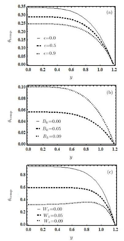
Figure 5 depicts the behavior of $\epsilon$, $Bk $ and $W_{z} $ on temperature. Here $\theta _{\rm temp} $ is plotted against $y$. Figure 5(a) shows that when $\theta _{\rm temp} $ decreases $\epsilon $ increases. While Figs. 5(b) and 5(c) show increase of $\theta _{\rm temp} $ as $Bk $ and $W_{z} $ increase.
Fig. 5
 New window|Download| PPT slide
Fig. 5(a) Influence of $\epsilon $ on $\theta _{\rm temp}$ for $Bk=0.1$, $e=0.6$, $x=0.2$, and $W_{z}=0.01$. (b) Influence of $Bk$ on $\theta _{\rm temp}$ for $W_{z}=0.01$, $e=0.6$, $\theta =1.1$, $x=0.2$, and $\alpha =0.1$. (c) Influence of $W_{z}$ on $\theta _{\rm temp}$ for $Bk=2$, $e=0.5$, $x=0.2$, $\theta =1.1$, and $\epsilon =0.1$.
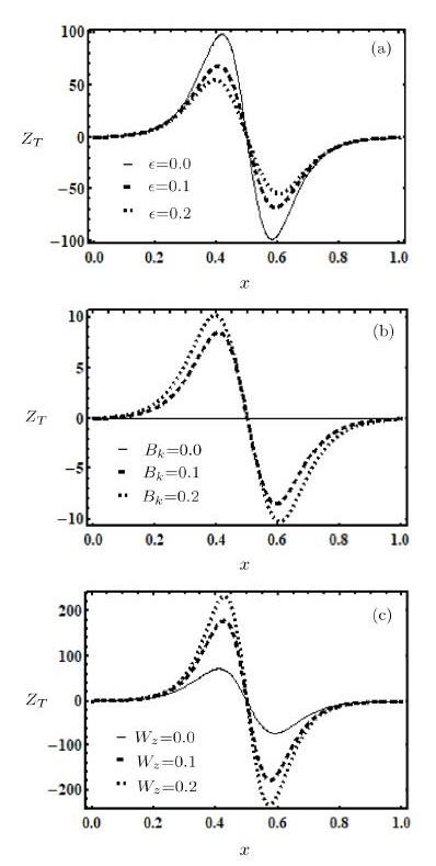
Figure 6 depicts the variation of heat transfer coefficient $Z_{T} $ for several values of parameters at $y=h(x)$. Figure 6(a) shows that as $\epsilon $ increases, the value of $Z_{T}$ decreases. Whereas in Figs. 6(b) and 6(c) $Z_{T} $ increases by increasing the values of $Bk$ and $W_{z}$.
Fig. 6
 New window|Download| PPT slide
Fig. 6(a) Influence of $\epsilon $ on $Z_{T}$ for $Bk=0.8$, $e=0.5$, $x=0.2$, $\theta =-1.5$, and $W_{z}=0.02$. (b) Influence of $Bk$ on $Z_{T}$ for $\epsilon $ $=0.8$, $e=0.5$, $x=0.2$, $\theta =-1.5$, and $W_{z}=0.02$. (c) Influence of $W_{z}$ on $Z_{T}$ for $Bk=0.8$, $e=0.5$, $x=0.2$, $\theta =-1.5$, and $\epsilon =0.02$.
Fig. 7
 New window|Download| PPT slide
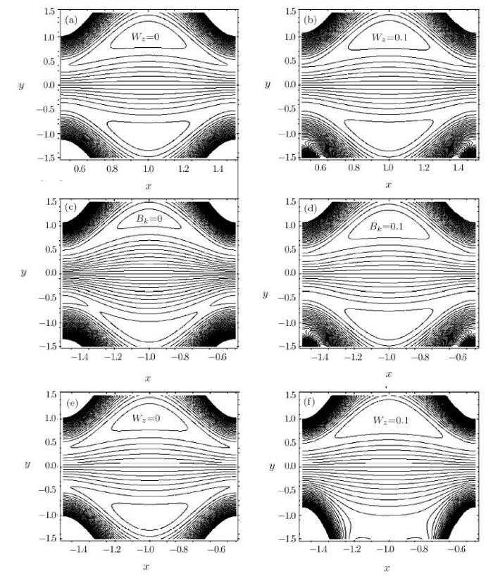
Fig. 7(a)--(b) Influence of streamlines for values of for $\epsilon =0$, 0.1, $Bk=0.2$, $e=0.5$, $W_{z}=0.01$, and $\theta =1.5$. (c)--(d) Influence of streamlines for values of for $Bk=0$, 0.1, $\epsilon =0.2$, $e=0.5$, $W_{z}=0.01$, and $\theta =1.5$. (e)--(f) Influence of streamlines for values of for $W_{z}=0$, 0.1, $Bk=0.2$, $e=0.5$, $\epsilon =0.01$, and $\theta =1.5$.
An important process in the transport of the fluid is trapping. Under some conditions, a bolus which is trapped is enclosed by the splitting of streamlines and it is carried out along the wave in the wave frame. The following process is known as trapping. Figure 7 represents the phenomenon of trapping by sketching streamlines. The bolus which is trapped, an increasing behavior is found, as the size of the bolus increases by increasing the parameters $\epsilon$, $Bk $, and $W_{z} $ respectively.
5 Conclusion
In the following paper we have examined the influence of variable fluid properties on peristaltic flow of Williamson fluid. By the help of perturbation method series solutions are found. The observations are concluded as follows:(i) It is observed that the behavior of $\epsilon $ on pressure gradient and pressure rise per wavelength, is opposite.
(ii) It is seen that $W_{z}$ and $\epsilon$, in the narrow part of the channel cause better variation as compared to the wider part of the channel.
(iii) As $W_{z} $ and $\epsilon$ increase, the pressure gradient decreases.
(iv) It is seen that when temperature increases thermal conductivity also increases whereas the temperature has negative relation with viscosity.
(v) The heat transfer coefficient is lower for a fluid with variable thermal conductivity and variable viscosity as compared to the fluid with constant thermal conductivity and constant viscosity.
(vi) When the values of $\epsilon $ and $W_{z}$ increase, the bolus which is trapped, its size increases.
Reference By original order
By published year
By cited within times
By Impact factor
[Cited within: 1]
[Cited within: 1]
[Cited within: 1]
DOI:10.1155/2014/426217URL [Cited within: 1]
DOI:10.1080/00986445.2011.586756URL [Cited within: 1]

The thermoconvective boundary layer flow of a generalized third-grade viscoelastic power-law non-Newtonian fluid over a porous wedge is studied theoretically. The free stream velocity, the surface temperature variations, and the injection velocity at the surface are assumed variables. A similarity transformation is applied to reduce the governing partial differential equations for mass, momentum, and energy conservation to dimensionless, nonlinear, coupled, ordinary differential equations. The homotopy analysis method (HAM) is employed to generate approximate analytical solutions for the transformed nonlinear equations under the prescribed boundary conditions. The HAM solutions, in comparison with numerical solutions (fourth-order Runge-Kutta shooting quadrature), admit excellent accuracy. The residual errors for dimensionless velocity and dimensionless temperature are also computed. The influence of the "power-law'' index on flow characteristics is also studied. The mathematical model finds important applications in polymeric processing and biotechnological manufacture. HAM holds significant promise as an analytical tool for chemical engineering fluid dynamics researchers, providing a robust benchmark for conventional numerical methods.
DOI:10.1016/j.asej.2015.08.012URL [Cited within: 1]
The purpose of this article is to study and analyze the convective flow of a third grade non-Newtonian fluid due to a linearly stretching sheet subject to a magnetic field. The dimensionless entropy generation equation is obtained by solving the reduced momentum and energy equations. The momentum and energy equations are reduced to a system of ordinary differential equations by a similarity method. The optimal homotopy analysis method (OHAM) is used to solve the resulting system of ordinary differential equations. The effects of the magnetic field, Biot number and Prandtl number on the velocity component and temperature are studied. The results show that the thermal boundary-layer thickness gets decreased with increasing the Prandtl number. In addition, Brownian motion plays an important role to improve thermal conductivity of the fluid. The main purpose of the paper is to study the effects of Reynolds number, dimensionless temperature difference, Brinkman number, Hartmann number and other physical parameters on the entropy generation. These results are analyzed and discussed.
DOI:10.1016/j.aej.2016.05.009URL [Cited within: 1]
The two-dimensional unsteady laminar free convective heat and mass transfer fluid flow of a non-Newtonian fluid adjacent to a vertical plate has been analyzed numerically. The two parameters Lie group transformation method that transforms the three independent variables into a single variable is used to transform the continuity, the momentum, the energy and the concentration equations into a set of coupled similarity equations. The transformed equations have been solved by the Runge–Kutta–Fehlberg fourth-fifth order numerical method with shooting technique. Numerical calculations were carried out for the various parameters entering into the problem. The dimensionless velocity, temperature and concentration profiles were shown graphically and the skin friction, heat and mass transfer rates were given in tables. It is found that friction factor and heat transfer (mass transfer rate) for methanol are higher (lower) than those of hydrogen and water vapor. Friction factor decreases while heat and mass transfer rate increase as the Prandtl number increases. Friction (heat and mass transfer rate) factor of Newtonian fluid is higher (lower) than the dilatant fluid.
[Cited within: 1]
DOI:10.1371/journal.pone.0129588URLPMID:4470995 [Cited within: 1]
In this paper, we study the influence of heat sink (or source) on the peristaltic motion of pseudoplastic fluid in the presence of Hall current, where channel walls are non-conducting in nature. Flow analysis has been carried out under the approximations of a low Reynolds number and long wavelength. Coupled equations are solved using shooting method for numerical solution for the axial velocity function, temperature and pressure gradient distributions. We analyze the influence of various interesting parameters on flow quantities. The present study can be considered as a mathematical presentation of the dynamics of physiological organs with stones.
[Cited within: 1]
DOI:10.1615/HeatTransRes.v47.i1URL [Cited within: 1]
DOI:10.1016/j.petrol.2013.05.010URL [Cited within: 1]
61The velocity field is retarded by the suction/injection Reynolds number.61The suction/injection Reynolds number retards the temperature.61The suction/injection Reynolds number increases the wall shear stress.61The Nusselt number is diminished by the suction/injection Reynolds number.61Possibility of blow up of solutions higher at larger suction/injection Reynolds numbers.
DOI:10.1140/epjp/i2014-14033-3URL [Cited within: 1]
http://link.springer.com/article/10.1140%2Fepjp%2Fi2014-14033-3
[Cited within: 1]
DOI:10.1016/j.rinp.2016.11.016URL [Cited within: 2]
This article addresses the impact of temperature dependent variable properties on peristaltic flow of third order fluid in a symmetric channel. The MHD fluid and viscous dissipation effects are taken into account. Assumptions of long wavelength and low Reynolds number are employed to model the problem. The governing nonlinear coupled equations are solved using perturbation method. Approximate solutions are obtained for the stream function, temperature and pressure gradient. The results are graphically analyzed with respect to various pertinent parameters.
DOI:10.1016/j.aej.2015.03.030URL [Cited within: 1]
Abstract In this article, a theoretical study is presented for peristaltic flow of a MHD fluid in an asymmetric channel. Effects of viscosity variation, velocity-slip as well as thermal-slip have been duly taken care of in the present study. The energy equation is formulated by including a heat source term which simulates either absorption or generation. The governing equations of motion and energy are simplified using long wave length and low Reynolds number approximation. The coupled non-linear differential equations are solved analytically by means of the perturbation method for small values of Reynolds model viscosity parameter. The salient features of pumping and trapping are discussed with particular focus on the effects of velocity-slip parameter, Grashof number and magnetic parameter. The study reveals that the velocity at the central region diminishes with increasing values of the velocity-slip parameter. The size of trapped bolus decreases and finally vanishes for large values of magnetic parameter.
DOI:10.18869/acadpub.jafm.68.228.24417URL [Cited within: 1]
DOI:10.1016/j.ijrmms.2006.07.003URL [Cited within: 1]
The Geological Strength Index (GSI) system, proposed in 1995, is now widely used for the estimation of the rock mass strength and the rock mass deformation parameters. The GSI system concentrates on the description of two factors, rock structure and block surface conditions. The guidelines given by the GSI system are for the estimation of the peak strength parameters of jointed rock masses. There are no guidelines given by the GSI, or by any other system, for the estimation of the rock mass' residual strength that yield consistent results. In this paper, a method is proposed to extend the GSI system for the estimation of a rock mass's residual strength. It is proposed to adjust the peak GSI to the residual GSI(r) value based on the two major controlling factors in the GSI system-the residual block volume V-b(r) and the residual joint condition factor J(c)(r). Methods to estimate the residual block volume and joint condition factor are presented. The proposed method for the estimation of rock mass's residual strength is validated using in-situ block shear test data from three large-scale cavern construction sites and data from a back-analysis of rock slopes. The estimated residual strengths, calculated using the reduced residual GSI(r) value, are found to be in good agreement with field test or back-analyzed data. (c) 2006 Elsevier Ltd. All rights reserved.
DOI:10.1016/j.trmi.2017.02.004URL [Cited within: 1]
The magneto hydrodynamic boundary layer flow with heat and mass transfer of Williamson nanofluid over a stretching sheet with variable thickness and variable thermal conductivity under the radiation effect is examined. It is assumed that the sheet is non-flat. The governing partial differential equations are reduced to nonlinear coupled ordinary differential equations by applying the suitable similarity transformations. These nonlinear coupled ordinary differential equations, subject to the appropriate boundary conditions, are then solved by using spectral quasi-linearisation method (SQLM). The effects of the physical parameters on the flow, heat transfer and nanoparticle concentration characteristics of the problem are presented through graphs and are discussed in detailed. Numerical values of skin friction co-efficient and Nusselt number with different parameters were computed and analysed.
[Cited within: 1]
DOI:10.1016/j.cnsns.2009.07.026URL [Cited within: 2]
In this work, we have presented a peristaltic flow of a Williamson model in an asymmetric channel. The governing equations of Williamson model in two dimensional peristaltic flow phenomena are constructed under long wave length and low Reynolds number approximations. A regular perturbation expansion method is used to obtain the analytical solution of the non-linear problem. The expressions for stream function, pressure gradient and pressure rise have been computed. The pertinent features of various physical parameters have been discussed graphically. It is observed that, (the non-dimensional Williamson parameter) for large We, the curves of the pressure rise are not linear but for very small We it behave like a Newtonian fluid. [All rights reserved Elsevier].
DOI:10.1016/j.mcm.2010.02.001URL [Cited within: 2]
In this paper the influence of inclined magnetic field on the peristaltic flow of a Williamson fluid in an inclined symmetric or asymmetric channel has been investigated initially in the wave frame of reference. The highly nonlinear equations are simplified under lubrication approach. The analytical and numerical solutions of the proposed problem have been computed and analyzed. The graphical results are displayed to see the effects of various physical parameters of interest.
[Cited within: 1]
DOI:10.1016/j.nonrwa.2012.04.008URL [Cited within: 1]
The peristaltic flow of a Williamson fluid in asymmetric channels with permeable walls is investigated. The channel asymmetry is produced by choosing a peristaltic wave train on the wall with different amplitudes and phases. The solutions for stream function, axial velocity and pressure gradient are obtained for small Weissenberg number, We, via a perturbation expansion about We, while an exact solution method is discussed for large values of We. The exact solutions become singular as We tends to zero; hence the separate perturbation solutions are essential. Also, numerical results are obtained using the perturbation technique for the pumping and trapping phenomena, and these are used to bring out the qualitative features of the solutions. It is noted that the size of the trapped bolus decreases and its symmetry disappears for large values of the permeability parameter. The effects of various wave forms (namely, sinusoidal, triangular, square and trapezoidal) on the fluid flow are discussed.
