Pavel V. Kostryukov ^1,
, Artur Dobrowolski ^1,
, Bo?ena Nerlo-Pomorska ^1,
, Micha? Warda ^1,
, Zhigang Xiao ^2,,
, Yongjing Chen ^3,
, Lile Liu ^3,
, Jun-Long Tian ^4,
, Krzysztof Pomorski ^1,,
,

Corresponding author: Zhigang Xiao, xiaozg@mail.tsinghua.edu.cn

Corresponding author: Krzysztof Pomorski, Krzysztof.Pomorski@umcs.pl

1.Institute of Physics, Maria Curie Sk?odowska University, 20-031 Lublin, Poland
2.Department of Physics, Tsinghua University, Beijing 100084, China
3.Institute of Atomic Energy, Beijing 102413, China
4.School of Physics and Electrical Engineering, Anyang Normal University, Anyang 455000, China
Received Date:2021-08-17
Available Online:2021-12-15
Abstract:Potential energy surfaces and fission barriers of superheavy nuclei are analyzed in a macroscopic-microscopic model. The Lublin-Strasbourg Drop (LSD) model is used to obtain the macroscopic part of the energy, whereas the shell and pairing energy corrections are evaluated using the Yukawa-folded potential; a standard flooding technique is utilized to determine barrier heights. A Fourier shape parametrization containing only three deformation parameters is shown to effectively reproduce the nuclear shapes of nuclei approaching fission. In addition, a non-axial degree of freedom is taken into account to better describe the structure of nuclei around the ground state and in the saddle region. In addition to the symmetric fission valley, a new highly asymmetric fission mode is predicted in most superheavy nuclei. The fission fragment mass distributions of the considered nuclei are obtained by solving 3D Langevin equations.

HTML

--> --> -->

Theoretical studies of the properties of superheavy nuclei (SHN) are of great importance as validation with experimental data offers a stringent test for any nuclear model. Most nuclear theories can produce a fair description of mass and other properties of nuclei near the $ \beta $-stability line; however, their predictions often deviate for nuclei far from stability, e.g., in the SHN region. The predictive power of these theoretical approaches not only aids in better understanding the relevant physics but also plays an essential role in guiding the challenging experimental quest for the so-called SHN island of stability and the limits of existence of bound nuclei.
Superheavy nuclei [1,2] with a charge number Z of up to 118 have been produced by two types of fusion reactions. The first is cold fusion at GSI, Germany [3,4], and RIKEN, Japan [5], which uses the doubly magic target $ ^{208} $Pb or its neighbour $ ^{209} $Bi; the second is hot fusion with the $ ^{48} $Ca projectile at JINR Dubna, Russia, and Livermore Nat. Lab., USA [6,7]. Further attempts to synthesize Z = 119,120 isotopes are in progress, (see [8,9]). Several theoretical studies were also performed in the past years to investigate the properties, possible decay modes, and fission fragment mass yields [10-16], as well as the synthesis possibility of nuclei in this region [17-20].
This study is a continuation of our work on the fission fragment mass yields of even-even Ra-Th and actinide nuclei [21-23], in which we presented a macroscopic-microscopic (mac-mic) model based on the Lublin-Strasbourg Drop (LSD) formula [24] and demonstrated that the Yukawa-folded single-particle potential [25] effectively describes fission barrier heights and fission fragment mass yields (FMY). In the present study, we aim to predict the fission barrier heights and FMY of SHN using the same set of model parameters. The calculation is performed in 4D Fourier deformation parameter space [26,27].
The Born-Oppenheimer+Wigner model used in Ref. [22] is not expected to describe a situation with two competing fission modes. Therefore, in this study, we evaluate FMY by solving 3D Langevin equations, similar to that in Ref. [23] done for some actinides. This alteration is because, in some isotopes of SHN, our mac-mic model predicts two well-separated fission valleys: one corresponding to symmetric fission and the other corresponding to asymmetric fission, which leads to heavy fragments around $ ^{208} $Pb.
This paper is organized in the following way. Section II presents details of the theoretical models used in the present study, Section III shows the collective potential energy surface evaluated within the mac-mic model for the selected isotopes and our fission barrier height estimates, Section IV contains the estimated FMY, and conclusions and perspectives from further investigations can be found at the end of the paper.

The potential energy surfaces (PES) of fissioning nuclei are studied within the mac-mic model in four-dimensional space built on deformation parameters describing the elongation, left-right asymmetry, neck, and non-axiality of the nucleus. A detailed study of the evaluated PES for SHN allows for the estimation of equilibrium deformations, possible shape coexistence and shape isomers, fission barrier height, and fission valleys. The dissipative fission dynamics of the obtained PES are described by Langevin equations, which estimate the possible fission modes and corresponding FMY. Below, we briefly present the main features of our model.
2

-->

A.Fourier nuclear shape parametrization

The axial symmetric shape-profile function of a fissioning nucleus written in cylindrical coordinates $ (\rho,z) $ is expanded in a Fourier series [26,27] as follows:

$\begin{aligned}[b] \frac{\rho^2_s(u)}{R_0^2} = & a_2\cos(u)+a_3\sin(2u)+a_4\cos(3u)\\& +a_5\sin(4u) + a_6\cos(5u)+\dots, \end{aligned} $

(1)

where $ R_0 $ is the radius of a spherical nucleus and $ u = $$ \pi/2\cdot(z-z_{\rm sh})/z_0 $ with $z_{\min} = -z_0+z_{sh}\leqslant z\leqslant z_0+z_{\rm sh} = z_{\max}$. The volume conservation condition gives $z_0 = R_0\pi/ $$ (a_2-a_4/3+a_6/5-\dots)/3$. The shift in the $ z $-coordinate $ z_{\rm sh} $ ensures that the centre of mass is located at the origin of the coordinate system. The Fourier expansion coefficients can be used as free deformation parameters, but it is more effective to combine them $ \{q_n\} $ into what are called optimal coordinates [27]:

$ \left\{ \begin{array}{ll} q_2 = a_2^{(0)}/a_2 - a_2/a_2^{(0)}\; ,& q_3 = a_3\; , \\[1ex] q_4 = a_4+\sqrt{(q_2/9)^2+(a_4^{(0)})^2}\; ,&\\[1ex] q_5 = a_5-(q_2-2)a_3/10\; ,& \\[1ex] q_6 = a_6-\sqrt{(q_2/100)^2+(a_6^{(0)})^2} &\;\;. \end{array} \right. $

(2)

The deformation parmeters $ q_n(\{a_i\}) $ were chosen in such a way that the liquid-drop energy as a function of elongation $ q_2 $ becomes minimal along a trajectory that defines the liquid-drop path to fission. The $ a^{(0)}_{2n} $ in Eq. (2) are the expansion coefficients of a spherical shape given by $ a^{(0)}_{2n} = (-1)^{n-1}32/\pi^3/(2n-1)^3 $. The optimal deformation parameters introduced in Eq. (2) have the following meaning: parameters $ q_2 $ and $ q_3 $ describe the elongation of the nucleus and its reflection asymmetry, respectively, $ q_4 $ is mainly responsible for the neck of the nucleus, and parameters $ q_5 $ and $ q_6 $ mainly regulate the deformation of fission fragments and the elongation of the neck.
Non-axial shapes can easily be obtained assuming that, for a given value of the $ z $-coordinate, the surface cross-section has the form of an ellipse with half-axes $ a(z) $ and $ b(z) $ [27]

$ \varrho^2(z,\varphi) = \rho^2_s(z) \frac{1-\eta^2}{1+\eta^2+2\eta\cos(2\varphi)} \quad {\rm with} \quad \eta = \frac{b-a}{a+b}\; , $

(3)

where the parameter $ \eta $ describes the non-axial deformation of nuclear shapes. The volume conservation condition requires that $ \rho_s^2(z) = a(z)b(z) $.
2 -->

B.Macroscopic-microscopic model

In the mac-mic method, first proposed by Myers and ?wi?tecki [28], the total energy of the deformed nucleus is equal to the sum of the macroscopic (liquid-drop type) energy and the quantum energy correction for protons and neutrons generated by shell and pairing effects

$ E_{\rm tot} = E^{}_{\rm LSD}+ { E_{\rm shell}} + { E_{\rm pair}} \; . $

(4)

The LSD model [24], which effectively reproduces all experimental masses and fission barrier heights, is used in this study to evaluate the macroscopic part of the energy. The shell corrections are obtained by subtracting the average energy $ \widetilde E $ from the sum of the single-particle (s.p.) energies of occupied orbitals

$ { E_{\rm shell}} = \sum\limits_k e_k - \widetilde E \; . $

(5)

For the s.p. energies $ e_k $, we use the eigenvalues of a mean-field Hamiltonian with the Yukawa-folded s.p. potential [25]. The average energy $ \widetilde E $ is evaluated using the Strutinsky prescription [29-32] with a 6$ ^{\rm th} $ order correction polynomial. The pairing energy correction is determined as the difference between the BCS energy [33] and the s.p. energy sum from which the average pairing energy [32] is subtracted

${E_{{\rm{pair}}}} = {E_{{\rm{BCS}}}} - \sum\limits_k {{e_k}} - {\tilde E_{{\rm{pair}}}}.$

(6)

In the BCS approximation, the ground-state energy of a system with an even number of particles is given by

$ E_{\rm BCS} = \sum\limits_{k>0} 2e_k v_k^2 - G\left(\sum\limits_{k>0}u_kv_k \right)^2 - G\sum\limits_{k>0} v_k^4 -{\cal E}_0^\varphi\;, $

(7)

where the sums run over the pairs of s.p. levels belonging to the pairing window defined below. The coefficients $ v_k $ and $ u_k = \sqrt{1-v_k^2} $ are the BCS occupation amplitudes, and $ {\cal E}_0^\varphi $ is the energy correction due to the particle number projection performed in the GCM+GOA approximation [34]

$ {\cal E}_0^\varphi = \frac{\displaystyle\sum\limits_{k>0}[ (e_k-\lambda)(u_k^2-v_k^2) +2\Delta u_k v_k +Gv_k^4] / E_k^2}{\displaystyle\sum\limits_{k>0} E_k^{-2}}\;. $

(8)

Here, $ E_k = \sqrt{(e_k-\lambda)^2+\Delta^2} $ are the quasi-particle energies, and $ \Delta $ and $ \lambda $ are the pairing gap and Fermi energy, respectively. The average projected pairing energy for a pairing window, symmetric in energy with respect to the Fermi energy, of width $ 2\Omega $, is equal to

$ \begin{aligned}[b] \tilde E_{\rm pair} =& {-\frac{1}{2}\,\tilde{g}\, \tilde{\Delta}^2+\frac{1}{2}\tilde{g}\,G\tilde{\Delta}\, {\rm arctan}\left(\frac{\Omega}{\tilde\Delta}\right) -\log\left(\frac{\Omega}{\tilde\Delta}\right)\tilde{\Delta}}\\& { +\frac{3}{4}G\frac{\Omega/\tilde{\Delta}}{1+(\Omega/\tilde{\Delta})^2}/ {\rm arctan}\left(\frac{\Omega}{\tilde{\Delta}}\right)-\frac{1}{4}G }\; , \end{aligned} $

(9)

where $ \tilde{g} $ is the average single-particle level density, and $ \tilde\Delta $ is the average pairing gap corresponding to a pairing strength $ G $

$ \tilde\Delta = {2\Omega\exp\left(-\frac{1}{G\tilde{g}}\right)}\; . $

(10)

The pairing window for protons or neutrons contains $ 2\sqrt{15\cal N} $ ($ \cal N = \, $N or Z) s.p. levels closest to the Fermi energy states. For such a window, the pairing strength approximated in Ref. [35] is given by the following expression:

$ G = {\frac{g_0}{{\cal N}^{2/3} \, A^{1/3}}}\; . $

(11)

The same value $ g_0 = g_0^p = g_0^n = 0.28 \hbar \omega_0 $ is taken for protons and neutrons, where $\omega_0 = 41$ MeV$ /A^{1/3} $ is the nuclear harmonic oscillator constant.
In our calculation, the single-particle spectra are obtained by diagonalization of the s.p. Hamiltonian with the Yukawa-folded potential [25,36] using the same parameters as in Ref. [37].
2 -->

C.Multidimensional Langevin equation

To study the fission dynamics of atomic nuclei, we use the Langevin equation formalism, which determines the motion of the nucleus in the multidimensional space of deformation parameters $ q_i $ (Eq. (2)). Such a system of coupled equations is similar to the canonical Hamilton equations with friction; however, this additionally contains a stochastic force. The Langevin equations can be written as follows (see Ref. [38]):

$ \left\{ \begin{aligned} {\dfrac{{\rm d}q_i}{{\rm d}t} = }& {\displaystyle\sum\limits_{j} \left[\mathcal{M}^{-1}\right]_{ij}p_j,}\\[3ex] {\dfrac{{\rm d}p_i}{{\rm d}t} = }& {-\dfrac{\partial V}{\partial q_i}-\dfrac{1}{2}\displaystyle\sum\limits_{jk} {\left[\dfrac{\mathcal{M}^{-1}}{\partial q_i}\right]_{jk}}p_jp_k} \\[3ex] & {+ \displaystyle\sum\limits_{jk}\gamma_{ij} \left[\mathcal{M}^{- 1} \right]_{jk}p_k + \sum_{j} g_{ij} \Gamma_j \; ,} \end{aligned} \right. \; $

(12)

where $ p_i $ is the conjugated momentum corresponding to the coordinate $ q_i $, $ \mathcal{M}_{ij}(q) $ and $ \gamma_{ij}(q) $ are the inertia and the friction tensors, respectively, and $ V(q) $ is the potential energy of the fissioning nucleus.
The inertia tensor is calculated within the incompressible and irrotational liquid drop model using the Werner-Wheeler approximation [39]. For the nuclear surface described by the function $ \rho^2_s(z,q) $ (Eq. (1)), the inertia tensor is given by the following formula [38]:

$ \mathcal{M}_{ij}(q) = \pi \rho_m \int\limits_{z_{\min}}^{z_{\max}} \rho^2_s(z,q) \left[ A_i A_j + \frac{1}{8}\rho^2_s(z, q )A_i' A_j' \right] {\rm d} z \; . $

(13)

Here, $ \rho_m = M_0/(\frac{4}{3}\pi R_0^3) $ is the density of nucleus and $z_{\min}$ and $z_{\max}$ are the $ z $-coordinates of both ends of the nucleus. The velocity expansion coefficients $ A_i $ in Eq. (13) have the following form:

$ A_i = \frac{1}{\rho^2_s(z, q)}\frac{\partial}{\partial q_i}\int_{z}^{z_{\max}} \rho^2_s (z', q) {\rm d}z' \; , $

(14)

and $ A_i' = \partial A_i/\partial z $.
During the fission process, the temperature of the nucleus changes due to the existence of friction forces. To take this effect into account, another type of the potential must be used, known as the temperature dependent Free Helmholtz energy $ F(q) $, instead of the temperature independent potential $ V(q) $ in the Langevin equation (12) (see [38]):

$ F(q) = V(q) - a(q)T^2\; ,$

(15)

where $ T $ is the temperature of the nucleus

$ T = \sqrt{E^*/a(q)}\; . $

(16)

Here, $ E^* $ is the thermal (statistical) excitation energy of the nucleus, and $ a(q) $ is the s.p. level density parameter. In our calculation, the parameter $ a(q) $ is taken from Ref. [40].
The collective potential in Eq. (4) in the mac-mic approximation is given by the sum of the macroscopic and the microscopic parts $ V = V_{\rm mac}+V_{\rm mic} $. The first term is almost temperature independent at low excitation energies, while the temperature dependence of the microscopic energy correction may be approximated as follows [40]:

$ V_{\rm mic}(q, T) = {\frac{V_{\rm mic}(q, T = 0)}{1 + e^{(1.5 - T)/0.3}}}\; . $

(17)

Also, the friction forces vary with temperature; they vanish in a cold system and grow with the excitation of the nucleus. We consider their temperature dependence using the following function:

$ \gamma^{\rm mic}_{ij} = {\frac{0.7\cdot\gamma^{\rm wall}_{ij}} {1+e^{(0.7-T)/0.25}}}\; , $

(18)

which approximates the estimates performed in Ref. [41]. Here, the friction tensor $ \gamma^{\rm wall}_{ij} $ is given by the wall-formula [42]

$ \gamma^{\rm wall}_{ij} = \frac{\pi}{2} \rho_m \bar{v} \int\limits_{z_{\min}}^{z_{\max}} \frac{\partial \rho^2_s}{\partial q_i} \frac {\partial \rho^2_s}{\partial q_j} \left[ \rho^2_s + \frac{1}{4} \left (\frac {\partial \rho^2_s}{\partial z} \right)^2 \right]^{-1/2} {\rm d}z,$

(19)

where $ \bar{v} $ is the average internal velocity of nucleons in the nucleus; its value is related to the Fermi velocity $ v_F $ as $ \bar{v} = \dfrac{3}{4} v_F $.
The final term of the second equation in Eq. (12) represents the random Langevin force. Its amplitude $ g_{ij} $ is the square-root of the diffusion tensor $ D_{ij} $ and $ \Gamma = \xi \cdot \sqrt{\tau} $, which is a time-dependent random function, where $ \xi $ is defined as a random Gaussian distribution with properties similar to those of white noise

$ \bar{\xi} = 0, \: \bar{\xi}^2 = 2\; , $

(20)

and $ \tau $ is the time step used when solving the Langevin equations.
The diffusion tensor is obtained using the Einstein relation

$ D_{ij} = \sum_k g_{ik} g_{jk} = \gamma_{ij} \cdot T\; , $

(21)

Unfortunately, the Einstein relation, which is valid for systems that have relatively high temperatures, does not take into account the quantum fluctuations present at low excitations of nuclei. To extend the application of the Langevin equations to low energy fission, the temperature $ T $ in Eq. (21) is replaced with the effective temperature $ T^* $ [43,44] as follows:

$ T^* = \frac{E_0}{2} \coth \frac{E_0}{2 T}\; , $

(22)

where $ E_0 $ corresponds to the zero-point energy of collective vibrations of the order 1$ \, $MeV.
The irrotational flow inertia tensor (Eq. (13)) and the wall friction tensor (Eq. (19)) are evaluated using the Fortran codes published in Ref. [45].

The nuclear potential energies of even-even superheavy nuclei are evaluated in the equidistant grid of 4D collective space built on the $ q_2, \; q_3, \; q_4 $, and $ \eta $ deformation parameters. The total energy function of a nucleus is obtained as described in Sec. II.B. As it is challenging to graphically present such a 4D object, in the following section, we will only show several selected 2D cross-sections of full PES.
In Appendix A, the cross-sections $ (q_2,\eta) $ (l.h.s. column) and $ (q_2,q_3) $ (r.h.s. column) of the 4D potential energy surface of elements Ds to Z = 120 are shown. For each element, five pairs of maps corresponding to different isotopes are displayed. To better understand the properties of the cross-sections presented in the Appendix, two cross-sections of the $ ^{304} $120 isotope are investigated below.
In the top panel of Fig. 1, the ($ q_2,\,\eta $) cross-section of the PES of $ ^{304} $120 nucleus is presented. Each energy point in the plot is minimized with respect to the neck parameter $ q_4 $. Solid green lines are drawn in the figure to guide the eye. The lines correspond to the approximate positions of the frequently used $ \beta $ and $ \gamma $ Bohr deformation parameters, which describe a spheroid [46]. Here, "approximate" is used as the shapes considered in this study are richer than the spheroidal. The lines $ \gamma = 30^{\rm o} $ and $ 150^{\rm o} $ correspond to the largest non-axial deformations, while $ \gamma = 0,\; 120^{\rm o} $ correspond to the prolate shapes of the nucleus and $ \gamma = 60^{\rm o} $ and $ 180^{\rm o} $ correspond to the oblate forms. In addition, the green dashed line shows the $ \gamma = 10^{\rm o} $ direction. To orient the reader with the elongation of the nucleus, the line corresponding to $ \beta = 0.3 $ is displayed. The bottom panel shows the cross-section $ (q_2,\,q_3) $ of the PES of $ ^{304} $120 for the axial symmetric case ($ \eta = 0 $). Each energy point on the map is minimized to $ q_4 $ deformation. The layers in both maps correspond to the total energy of the nucleus, measured relative to the LSD energy spherical nucleus. The distance between the solid line layers is 2$ \, $MeV, while the dotted lines correspond to the half-layers.
Figure1. (color?online)?Potential energy surface of $ ^{304} $120 isotope minimized with respect to $ q_4 $ at $ (q_2,\eta) $ (top) and $ (q_2,q_3) $ (bottom). The lines corresponding to $\gamma\, = \,10^{\rm o},\,30^{\rm o}, $$ 60^{\rm o},\,120^{\rm o}$, and $ 150^{\rm o} $, as well as the line corresponding to $ \beta $ = 0.3, are marked in the $ (q_2,\eta) $ maps.

The nucleus $ ^{304} $120 is spherical in the ground-state and possesses two oblate shape isomers of comparable energies; shape coexistence is also suggested. The least energy path to fission reminds the situation observed in rotating nuclei [47]. First, it becomes oblate and then undergoes fission via triaxial shapes. The effect of a non-axial degree of freedom ceases around $ q_2 = 0.8 $ and $ \eta = 0.12 $ (or $ \gamma = 10^{\rm o} $). At larger deformations, the $ \eta $ degree of freedom does not play an essential role; therefore, it can be omitted when fission dynamics are discussed. The fission barrier reduction due to the breaking of the axial symmetry in $ ^{304} $120 is approximately 3 MeV.
In the bottom panel of Fig. 1, the $ (q_2,\,q_3) $ cross-section of the PES of $ ^{304} $120 is shown. Taking into account the left-right (octupole like) asymmetry diminishes the fission barrier of $ ^{304} $120 by approximately 1 MeV. At smaller elongation $ q_2<0.3 $, the minimum energy corresponds to $ q_3 = 0 $. Beyond the saddle point at $ (q_2\approx 0.4,\,q_3\approx 0.13,\,\eta\approx 0.14) $, the role of the octupole deformation becomes more important. Two fission valleys are formed with growing elongation of the nucleus. The first is left-right symmetric ($ q_3 = 0) $, which goes through a local minimum at $ q_2\approx 0.5 $ and ends at scission at $ q_2\approx 2.3 $, giving the symmetric in mass fission fragment distribution. The second valley for $ q_3\approx 0.2 $ causes highly asymmetric fission with the masses of the heavy fragments concentrated around A = 208. This is the effect of the double magic $ ^{208} $Pb. The potential existence of such a decay mode of SHN was also predicted by Poenaru et al. [48] and Warda and co-workers [49] as a cluster emission. Additionally, Ref. [49] shows that such a mode may be treated as super-asymmetric fission.
The maps presented in the Appendix for $ ^{254-262} $Rf, $ ^{258-266} $Sg, $ ^{264-272} $Hs, $ ^{276-284} $Ds, $ ^{278-286} $Cn, $ ^{282-290} $Fl, $ ^{286-294} $Lv, $ ^{290-298} $Og, and $ ^{294-302} $120 effectively illustrate the interplay between the non-axial and left-right asymmetric deformations of fissioning super-heavy nuclei. This is only a selection of similar results that we have obtained for 18 even-even isotopes chains of each element with 104$\leqslant$Z$ \leqslant $126. It is seen in Figs. A1-A9 that at elongations $ q_2\gtrapprox 0.8 $, the axially symmetric shape is the preferable shape of fissioning nuclei. Hence, the non-axial deformation should not influence further fission dynamics toward scission configuration. This justifies using only 3D deformation parameter space when finding the Langevin trajectories that lead to various scission points corresponding to the different masses of the fission fragments. Investigating such a broad range of superheavy isotopes is not only interesting from the point of view of their possible synthesis but also important for astrophysical models (see Refs. [50-52]).
FigureA1. (color?online)?Potential energy surface of $ ^{254-262} $Rf minimized with respect to $ q_4 $ at $ (q_2,\eta) $ (l.h.s. column) and $ (q_2,q_3) $ (r.h.s. column). The lines corresponding to $ \gamma\, = \, 10^{\rm o},\,30^{\rm o},\,60^{\rm o},\,120^0 $, and $ 150^{\rm o} $ as well as the line indicating $ \beta $ = 0.3 deformation are marked in the $ (q_2,\eta) $ maps.

FigureA2. (color?online)?The same as in Fig. A1 but for $ ^{258-266} $Sg isotopes.

FigureA3. (color?online)?The same as in Fig. A1 but for $ ^{264-272} $Hs isotopes.

FigureA5. (color?online)?The same as in Fig. A1 but for $ ^{} $Cn isotopes.

FigureA6. (color?online)?The same as in Fig. A1 but for $ ^{282-290} $Fl isotopes.

FigureA7. (color?online)?The same as in Fig. A1 but for $ ^{286-294} $Lv isotopes.

FigureA8. (color?online)?The same as in Fig. A1 but for $ ^{290-298} $Og isotopes.

FigureA9. (color?online)?The same as in Fig. A1 but for $ ^{294-302} $120 isotopes.

As a regular article does not contain sufficient space to discuss the details of the $ (q_2,\,q_3 ) $ and $ (q_2,\,\eta) $ maps for each isotope, we only systematically present their fission barrier heights in Fig. 2.
Figure2. (color online) Fission barrier heights of even-even superheavy nuclei evaluated in our 4D mac-mic model. The ground-state energy for Rf isotopes is taken as zero, while for each subsequent element, it is shifted by 2 MeV. The barrier plots are also shifted by the same amount. The ground state energy values corresponding to each element are marked on the r.h.s. vertical scale. The experimental data for the lower limit of the barrier heights [53] are marked by crosses and arrows of the same colors as the element symbols.

The barrier heights are evaluated using the flooding technique in 4D space. The results for each element, starting from Rf to Z = 120, are indicated by different colors. The ground-state energy for Rf isotopes is taken as to zero, and for each subsequent element, this is shifted by 2 MeV. In other words, one has to subtract $ (Z\,-\,104) $ MeV from the displayed value of the barrier height of element Z. Alternatively, the difference between the ground state energy (indicated by the dashed line of the same color) of each element and an appropriate solid curve can be observed.
The maximum barrier height for each element varies; this value is 7 MeV for Rf to Ds nuclei, reaches 9 MeV for $ ^{294} $Fl, and then decreases for elements up to Z = 120, which has an upper value of approximately 5 MeV. Following this, the effect of the semi-magic proton number appears, and the barrier height grows with the Z number, reaching a value 3.76 MeV for the hypothetical isotope $ ^{304} $126. A good comparison between the fission barrier heights evaluated in different mac-mic and self-consistent models for three selected superheavy elements is presented in Fig. 11 of Ref. [54]. Comparing the barrier heights shown in Fig. 2 with those reported in Ref. [52] shows that our estimates of the barrier heights for Cn isotopes differ from the finite range liquid droplet model (FRLDM) results [55] by approximately $ \pm 0.5 $ MeV. Furthermore, they are approximately 2 MeV higher than the mac-mic Woods-Saxon (WS) findings presented in Ref. [56]. The self-consistent estimates for Cn isotopes obtained in the SkM$ ^* $ [57] and NL3 [58] models are approximately 1 MeV and 3–4 MeV below the present results, respectively. However, this tendency changes when elements with higher charge numbers are examined. Therefore, in the case of Fl (Z = 114) isotopes, our estimates are close to the results obtained in FRLDM ($ \pm $1 MeV) and are approximately 3 MeV higher than those obtained in the WS model. Both self-consistent models predict lower barriers. Those obtained with SkM$ * $ forces are approximately 1.5 MeV lower, while the relativistic model with NLS parameters predicts barriers that are approximately 5 MeV lower than our estimates. The barrier heights for the hypothetical element with Z = 120, estimated in different models, are the highest for the SkM$ * $ force (8–10 MeV) and the lowest for NL3 (3–5 MeV). Our estimates for these isotopes are the closest to those obtained in the WS model and are approximately 2 MeV lower than the optimistic predictions of the FRLDM model.
A question to consider is whether our 4D deformation space ($ q_2,\,q_3,\,q_4,\,\eta $) is sufficient to describe the fission barriers and valleys as several other researchers have taken into account more deformation parameters to obtain similar results (see Ref. [13]). It is shown in Refs. [27,59] that the 4D Fourier shape parametrization used in this study effectively describes the main features of the potential energy of fissioning nuclei. The influence of the higher order Fourier expansion terms on the estimates of PES of fissioning actinide nuclei was studied in Ref. [59], which found that this effect is rather small. In the superheavy region of nuclei, changes in PES due to the $ q_5 $ and $ q_6 $ deformations are not large, even at nucleus elongations close to the scission configuration. Fig. 3 shows the ($ q_3,\,q_4 $) cross-section of the PES of $ ^{284} $Cn at the significant elongation $ q_2 = 2.1 $. The upper panel corresponds to the case in which the deformations $ q_5 $ and $ q_6 $ are not taken into account, while the bottom panel shows the PES minimized by these high order deformations. The shapes of the nucleus in the local minima are also shown in the upper panel. Comparing both maps in the vicinity of the minimum at $ q_3 = 0 $ and $ q_4 = -0.13 $, corresponding to the symmetric fission valley, the PES are shown to be almost unchanged. Some effect of $ q_5 $ and $ q_6 $ is seen around the local minimum at $ q_3 = 0.23 $ and $ q_4 = -0.13 $, corresponding to the highly asymmetric fission valley. Considering the $ q_5 $ and $ q_6 $ deformations broadens this minimum and reduces the barrier height separating both minima.
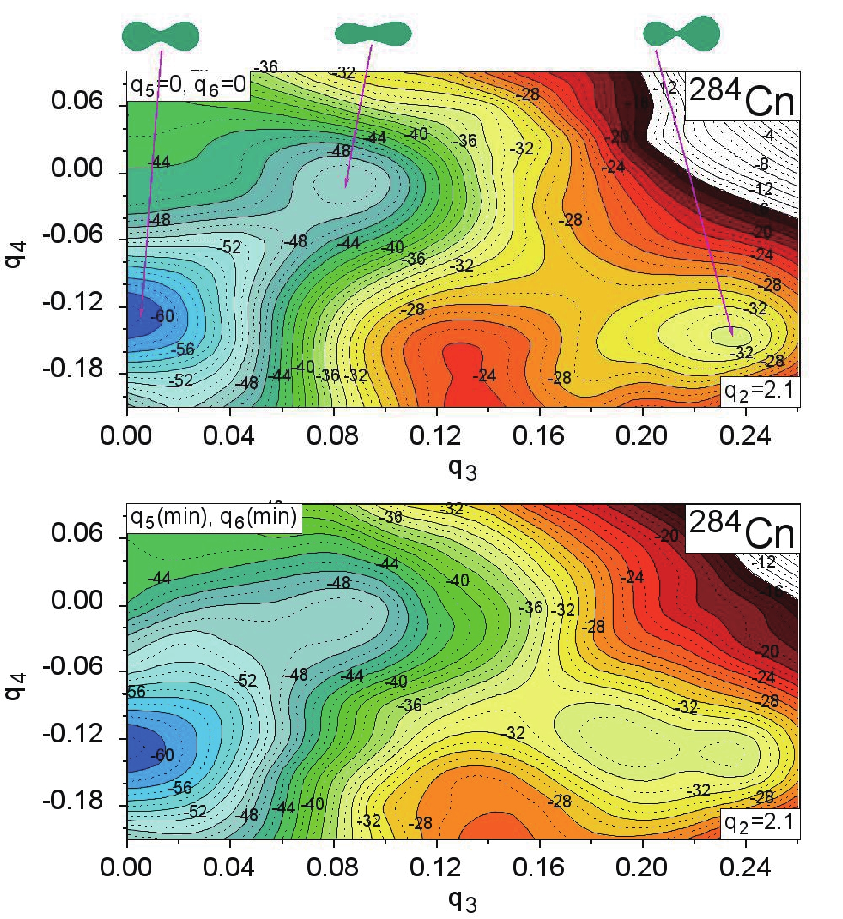Figure3. (color?online)?The $ (q_3,q_4) $ cross-section of the PES of $ ^{284} $Cn taken at the elongation $ q_2 = 2.1 $. The upper plot corresponds to the case in which the higher order deformations are not taken into account, while the bottom panel shows the PES minimized with respect to $ q_5 $ and $ q_6 $.

The PES cross-section of $ ^{284} $Cn, corresponding to the minimal energy as a function of $ q_3 $ for the constant elongation $ q_2 = 2.1 $, is presented in Fig. 4. The thick violet line corresponds to the case in which each point of the curve is minimized with respect to $ q_4 $, $ q_5 $, and $ q_6 $, while the thin green line shows the potential energy when the effect of $ q_5 $ and $ q_6 $ is neglected. The influence of the higher-order deformations on the energy values in the minima is barely observed.
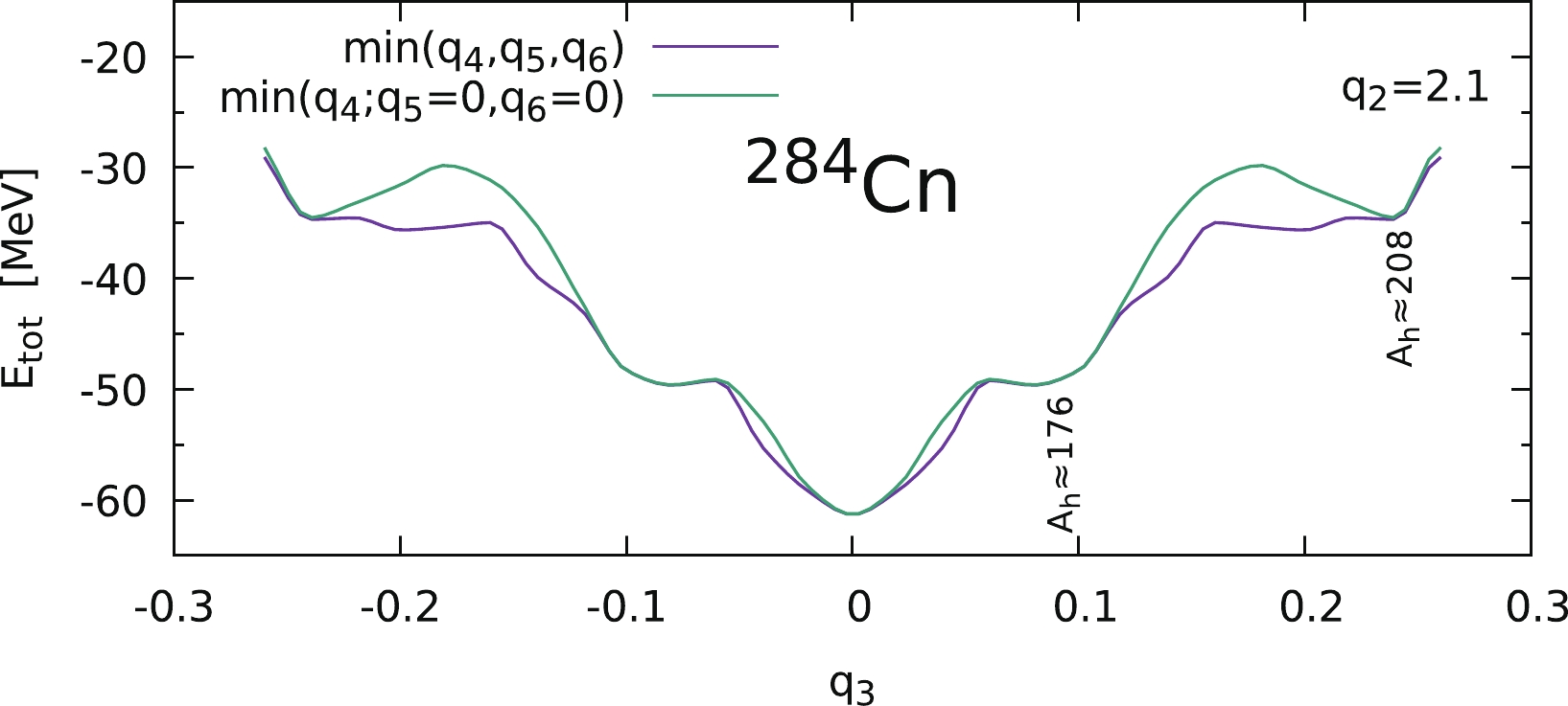Figure4. (color?online)?PES cross-section corresponding to the elongation $ q_2 = 2.1 $ as a function of the $ q_3 $ deformation. The thick violet line corresponds the PES minimized with respect to $ q_4 $, $ q_5 $, and $ q_6 $, while the thin green line indicates the case in which $ q_5 $ and $ q_6 $ are not considered.

Our group presented similar estimates of the SHN barrier height in Ref. [60]. The main difference between those and the present results originates mainly from a better and more accurate description of the pairing correlation effect (see Eqs. (7)–(9)), as well as using a denser and more extended 4D mesh in the deformation parameter space.

Having introduced the details of generating PES, we may switch to the statistical approach based on the Langevin formalism to find the fragment mass distributions of fissioning nuclei. The set of coupled Langevin equations defined in the Fourier deformation space, which leads to a bundle of stochastic trajectories between the ground state and a scission configuration on the scission surface, has previously been described in Subsection II.C.
All deformation dependent transport coefficients in Eq. (12) were stored for each nucleus at equidistant ($ \Delta q_2 = 0.05,\Delta q_3 = 0.03,\,\Delta q_4 = 0.03 $) mesh points in the 3D Fourier deformation parameters space. The values of the PES and the transport function and their derivatives between grid points are obtained using the Gauss-Hermite approximation method [61]. The non-axial degree of freedom $ \eta $ in Eq. (3) is not taken into account as its contribution at a large nuclear elongation is negligible.
The Langevin calculation of each $ n^{\rm th} $ trajectory begins at a starting point $ \{q^{\rm start}_n\} $. As the starting point can be chosen, to some extent, arbitrarily, a natural question arises: Which configuration should be taken as the beginning of the trajectories? Should it be the location of the ground state, the first or second saddle point, or the exit-point after tunneling of the potential energy barrier in the spontaneous fission case? To answer these questions, we discuss the following two types of starting points: those around the highest saddle and those at the exit point after quantum mechanical tunneling of the fission barrier. Both choices roughly correspond to neutron-induced fission and spontaneous fission, respectively. We are allowed to treat such a low energy system with Langevin type dynamics since instead of the thermodynamical temperature used in the Einstein relation Eq. (21), we take $ T^* $ (Eq. (22)), which roughly describes the effect of quantum mechanical fluctuations when $ T\rightarrow 0 $ [43,44]. Because the initial configuration cannot be sharp, we assume that the beginning of each Langevin trajectory will be randomly distributed around the starting point; the elongation $ q^{\rm start}_2 $ remains constant, and $ q_3 $ and $ q_4 $ and their conjugate momenta $ p_2,\,p_3 $, and $ p_4 $ are assumed to be randomly distributed around their starting value with the following condition:

$ \begin{aligned}[b] E_{\rm coll} =& {V(q_3,q_4;q^{\rm start}_2)-V(q^{\rm start}_3,q^{\rm start}_3; q^{\rm start}_2)}\\&+ {\frac{1}{2}\sum\limits_{i = 3,4;j = 3,4}{\cal M}_{ij}p_ip_j = E_0} \; , \end{aligned} $

(23)

which ensures the same initial collective energy ($ E_{\rm coll} $) in each random trajectory. Here, $ E_0 $ is the so-called zero-point energy, equal to 1 MeV in our calculation. The system of Langevin equations has been solved using a discretization method in the time variable.
The Langevin trajectory proceeds randomly towards fission within the following rectangular 3D box with the collective variables:

$ \begin{aligned}[b] q^{\rm start}_2 \leqslant & q_2 \\ -0.27\leqslant & q_3 \leqslant 0.27\\ -0.21 \leqslant & q_4 \leqslant 0.21 \end{aligned} $

(24)

with reflective walls that ensure none of the trajectories will escape before reaching the scission configuration at larger elongations $ q_2 $. Because the box (Eq. (24)) is sufficiently large, sticking of the walls occurs very rarely. A given trajectory ends when the neck radius of the fissioning nucleus reaches values of approximately 1 fm, which roughly corresponds to the "size" of a nucleon. The time-step when solving Langevin equations is taken to be $ \Delta\tau = 0.01\hbar/{\rm MeV}\approx\dfrac{2}{3}10^{-23} $ s. Typically, 20,000 trajectories have to be generated to obtain sufficiently smooth fission fragment mass yields, as presented in Figs. 6-8.
Figure6. (color online) Fission fragment mass yields of six Ds isotopes. The l.h.s. column corresponds to the case in which the Langevin trajectories begin in the vicinity of the saddle point (low energy fission), while the r.h.s. columns present the estimates made for the spontaneous fission when the trajectories begin around the exit point from the barrier.

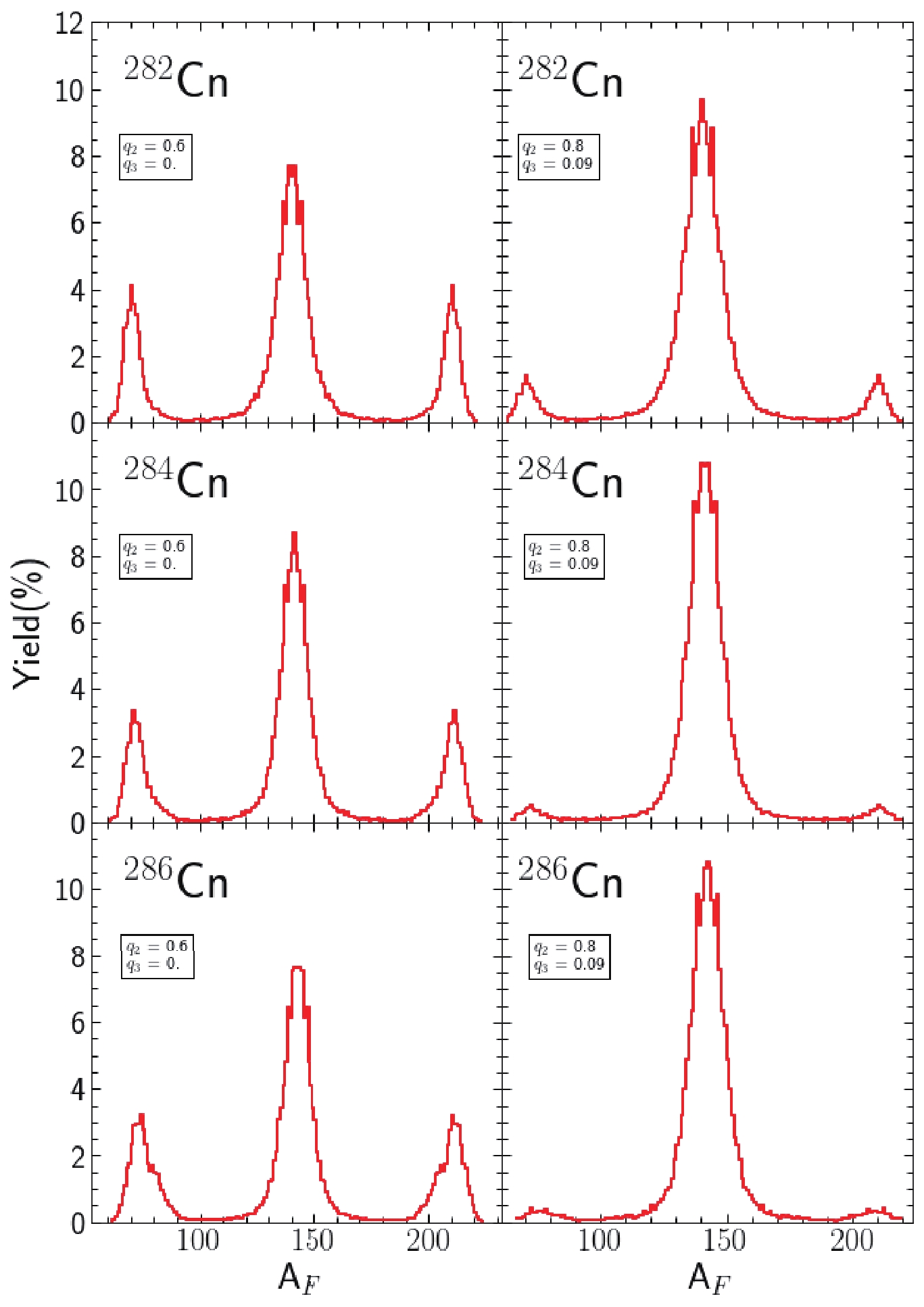Figure7. (color?online)?The same as in Fig. 6 but for Cn isotopes.

Figure8. (color?online)?The same as in Fig. 6 but for Fl isotopes.

Our Langevin estimates of the fission fragment mass yields of $ ^{262} $Rf are compared in Fig. 5 with empirical data taken from Ref. [62]. The agreement between the two is satisfactory and none of the model parameters have been ''tuned'' to this data set in the region of SHN. It should be noted that their values are the same as those produced from calculations for actinide nuclei. This proves that the choice of Langevin calculation parameters is reasonable and is expected to provide realistic estimates for the heavier nuclei presented below. The predicted small splitting of the symmetric peaks visible in Fig. 5 originates from a tiny light asymmetric valley ($ q_3 \approx $ 0.03), which is visible in the ($ q_2,\,q_3 $) PES of the lighter Rf isotopes in Fig. A1 (r.h.s. column).
Figure5. (color online) Fission fragment mass yield (red solid line) estimate for the $ ^{262} $Rf nucleus. The experimental (in the spontaneous fission case) data (black triangles) are taken from Ref. [62].

In Fig. 6, the fission fragment mass yields of the $ ^{270-282} $Ds isotopes are displayed. More precisely, these are pre-fission yields, i.e., the mass distribution before neutron emission. The l.h.s. column shows the yields corresponding to the case in which the saddle point is taken as the starting point, while the r.h.s panel represents the mass yields when the exit point from the fission barrier was used as the starting point. In this calculation and in the results presented in Figs. 7 to 8, the initial temperature of the fissioning nucleus is assumed to be zero ($ T = 0 $), independent of the starting point. The cases presented in the l.h.s. columns roughly correspond to neutron-induced fission, while those in the r.h.s. columns correspond to spontaneous fission. In all the figures, the symmetric fission peaks dominate; however, two smaller peaks corresponding to highly asymmetric fission, with a heavier fragment mass around A = 208, are also visible. The asymmetric peaks are significantly smaller when the exit from the barrier (i.e., the spontaneous fission case) was taken as the starting point. This property of FMY is unsurprising because the higher excitation energy accumulated in the potential energy of the nuclear system offers a relatively larger probability of penetrating more exotic shape configurations that are exhibited in the peripheries of PES. It must be stressed that the highly asymmetric peaks in the predicted fission fragment mass yields originate from the shell structure of the microscopic energy rather than fission dynamics, which is mainly responsible for the peak widths. The effect of the near double-magic heavy fission fragment is already visible at the elongations $ q_2\approx 1.2 $ and $ q_3\approx 0.21 $, as shown in the PES in Fig. A4.
FigureA4. (color?online)?The same as in Fig. A1 but for $ ^{276-284} $Ds isotopes.

Figures 7 and 8 show similar estimates of the FMY for the $ ^{282-286} $Cn and $ ^{286-292} $Fl isotopes. Symmetric fission also dominates in these isotopes; however, the contribution of the highly asymmetric component becomes large (up to 40 % trajectories for Fl) when the Langevin trajectories begin around the saddle point. Moreover, in spontaneous fission, four times fewer trajectories lead to the asymmetric valley. Our estimates are in line with results obtained in Ref. [12], where the 4D two-center shell model was used to evaluate the potential energy surfaces.

Properties of superheavy elements with a charge number of 104$ \leqslant $Z$ \leqslant $126 were studied within the mac-mic model in 4D Fourier deformation parameter space. All parameters for these calculations are kept unchanged because they effectively reproduce the empirical masses and fission barrier heights of nuclei from different mass regions.
The potential energy surfaces of 18 even-even isotope chains of elements from Rf to Z = 126 have been carefully studied, and the flooding technique was used to determine the fission barrier heights. An essential role of the non-axial and left-right asymmetry degrees of freedom was shown when evaluating the barrier heights. The minimum energy path to fission of the heaviest spherical and oblate nuclei from this region goes frequently via highly oblate and then non-axial shapes, leading to a significant decrease in their barrier heights.
A detailed investigation of PES suggests that the dominant fission channel of SHN (apart from the lightest isotopes of Rf to Hs) is symmetric. In addition, in nuclei with A$ \geqslant $280, another highly asymmetric fission channel appears, leading to a heavy fragment with mass A$ \approx $208. This effect suggests that the probability of synthesis of elements with Z$ \geqslant $118 is low.
At larger elongations ($ q_2\geqslant 0.8 $), the non-axial deformation may be neglected as the nucleus' minimal energy configurations always become axially symmetric. Therefore, in our dissipative dynamics calculation, this deformation mode is not considered, and the Langevin equations are solved in 3D space containing the elongation ($ q_2 $), neck ($ q_4 $), and mass asymmetry ($ q_3 $) degrees of freedom. Such a model effectively describes the main features of the fission fragment mass yields of superheavy nuclei. It was shown that adding higher-order terms ($ q_5,\,q_6 $) in the Fourier expansion (Eqs. (1), (2)) does not significantly change the properties of PES. The Langevin calculation allowed an estimation of the interplay between the symmetric and highly asymmetric fission modes of SHN. We have shown that, in spontaneous fission, the fraction of trajectories leading to a heavy fragment with a mass around A = 208 is a couple of times smaller than in the case of, e.g., neutron-induced fission in which the Langevin trajectories begin in the vicinity of the saddle point. Both fission valleys, symmetric and highly asymmetric, are well separated at a larger elongation ($ q_2 $) of the nucleus.

In Figs. A1-A9, we present the ($ q_2,\eta $) (l.h.s. columns) and ($ q_2,q_3 $) (r.h.s. columns) cross-sections of the 4D potential energy surfaces of five selected even-even isotopes of elements with a charge number 104$ \leqslant $Z$ \leqslant $120. These plots can be useful for researchers studying this nuclear region; however, they are merely 2D cross-sections and do not fully reflect the richness of 4D PES. Nevertheless, several main features can be seen, such as the location of the ground state, shape isomers, possible shape coexistence, and different paths to fission. In Sec. III, we described in detail the cross-sections of the $ ^{304} $120 nucleus with an explanation of the different curves presented in these maps; therefore, these explanations will not be repeated here.
As seen in Figs. A1-A3, all shown isotopes of Rf, Sg, and Hs are prolate in the ground-state. This is due to the deformed shell effect previously reported in 1990 by Patyk and Sobiczewski [63]. The microscopic energy correction in the ground-state is approximately –3 MeV in Rf isotopes, and becomes larger in Sg nuclei, reaching –4.5 MeV for $ ^{266} $Sg. The deformed shell energy effect in heavier Hs isotopes exceeds –5 MeV. In Ds nuclei, one observes the decrease in the prolate deformation and the appearance of gamma-instability in the ground state of $ ^{280} $Ds and heavier Ds isotopes. At the same time, the microscopic energy correction exceeds –4 MeV in these nuclei. The $ ^{278-286} $Cn are typical transitional nuclei with very flat PES around the spherical shape. In the $ ^{286} $Cn isotope, the triaxial shape ($ \gamma\approx 30^{\rm o} $) is preferred in the ground state. In Rf to Cn nuclei, the axial ($ \gamma = 0 $) and non-axial ($ \gamma\approx 30^{\rm o} $) paths to fission compete. The reduction of the saddle point energy due to non-axial deformation is less than 1 MeV in Rf isotopes and approximately 2 MeV in $ ^{258} $Sg. In $ ^{262-266} $Sg and all presented Hs isotopes, the axially symmetric and the non-axial fission barrier are comparable. In Ds and Cn isotopes, non-axial shape isomers appear at $ q_2\approx 0.6 $ and $ \eta\approx 0.1 $ (or $ \gamma = 10^{\rm o} $), and the axial and non-axial saddles have comparable energies. In Fl isotopes, the situation is similar; however, due to the left-right asymmetry ($ q_3 $) degree of freedom, the outer barrier of the non-axial isomers is diminished, and hence, they do not have a chance to be populated. In the $ ^{288-290} $Fl, Lv, Og, and Z = 120 isotopes, the path to fission leads from at the spherical or nearly spherical ground-state via oblate shapes and a non-axial saddle to highly elongated prolate deformations. A significant reduction (up to 3 MeV in $ ^{296-302} $120 nuclei) of the saddle point energy due to the $ q_3 $ deformation is observed in Lv and heavier elements. In addition to the symmetric fission valley ($ q_3\approx 0 $), a highly asymmetric valley ($ q_3\approx 0.22 $) appears in Ds and heavier elements.