Department of Physics, Sardar Vallabhbhai National Institute of Technology, Surat- 395007, Gujarat, India Received Date:2021-02-10 Available Online:2021-06-15 Abstract:The present study is dedicated to light-strange $\Lambda$ with strangeness S = ?1 and isospin I = 0, $\Sigma$ with S = ?1 and I = 1, and $\Xi$ baryon with S = ?2 and $I=\dfrac{1}{2}$. In this study, the hypercentral constituent quark model with linear confining potential has been employed along with a first order correction term to obtain the resonance masses up to approximately 4 GeV. The calculated states include 1S-5S, 1P-4P, 1D-3D, 1F-2F, and 1G (in a few cases) along with all possible spin-parity assignments. Regge trajectories have been explored for the linearity of the calculated masses for $(n,M^{2})$ and $(J,M^{2})$. Magnetic moments have been intensively studied for ground state spin $\dfrac{1}{2}$ and $\dfrac{3}{2}$, in addition to the configuration mixing of the first negative parity state for $\Xi$. Lastly, the transition magnetic moments and radiative decay widths have been presented.
HTML
--> --> -->
I.INTRODUCTIONThe objective of the study of hadrons is to reveal the possible degrees of freedom responsible for the appearance of a given system. The quark confinement and asymptotic freedom have been the starting points of any theoretical and phenomenological study to understand quark dynamics. Hadron spectroscopy attempts to explore the excited mass spectrum along with the multiplet structure and spin-parity assignments. The light quark baryons form the basis of octets and decuplets ranging from strangeness S = 0 to S = ?3 based on symmetric, asymmetric, and mixed-symmetric flavor-spin combinations.
The presence of a strange quark in a baryon draws attention because it would be slightly heavier than u and d quarks and considerably lighter than c and b quarks. Particularly, the strangeness S = ?2 $ \Xi $ baryons have not been observed experimentally like other light sector baryons [1], as depicted in Table 1. The limited observations in the $ \Xi $ baryon group are owing to the fact that they are produced only as the final state in a process in addition to having considerably small cross-sections [2]. Unlike the $ \Xi $ baryons, $ \Sigma $ and $ \Lambda $ with S = ?1 have quite a number of experimentally established states.
State
$J^{P}$
Status
$\Xi^{0}$(1314)
$\dfrac{1}{2}^{+}$
****
$\Xi^{-}$(1321)
$\dfrac{1}{2}^{+}$
****
$\Xi$(1530)
$\dfrac{3}{2}^{+}$
****
$\Xi$(1620)
*
$\Xi$(1690)
***
$\Xi$(1820)
$\dfrac{3}{2}^{-}$
***
$\Xi$(1950)
***
$\Xi$(2030)
$\dfrac{5}{2}^{?}$
***
$\Xi$(2120)
*
$\Xi$(2250)
**
$\Xi$(2370)
**
$\Xi$(2500)
*
Table1.$\Xi$ listed by Particle Data Group (PDG [1]).
The present article is dedicated to the study of $ \Lambda $, $ \Sigma $ and $ \Xi $ baryons. Cascade baryons appear with isospin $ I = \dfrac{1}{2} $ in the octet ($ J = \dfrac{1}{2} $) and decuplet ($ J = \dfrac{3}{2} $) as $ \Xi $ and $ \Xi^{*} $, respectively. The quark combination is uss for $ \Xi^{0} $ and dss for $ \Xi^{-} $. For mixed symmetry flavor wave-function in the octet group,
Similarly, the $ \Sigma $ baryon with u, d, and s constituent quarks has a place in octets and decuplets with three possible combinations as uus, uds, and dds respectively. The $ \Lambda $ baryon appearing in an octet as I = 0 has uds quark content; however, its wave-function differs from that of $ \Sigma^{0} $. Experimental facilities around the world have been striving to study strange hyperons. A recent study at CERN by ALICE Collaboration established an attractive interaction between protons and $ \Xi^{-} $ [3]. Activities in measuring weak decays of $ \Xi $ hyperons were reported by the KTeV Collaboration [4] and the NA48/1 Collaboration [5]; the BABAR Collaboration has also been carrying out extensive studies [6]. The photoproduction of $ \Xi $ has been observed by CLAS detector at Jefferson Lab [7]. Additionally, JLab has recently proposed to explore the strange hyperon spectroscopy through a secondary KL beam along with a GlueX experiment [8], and the findings are expected to provide new direction and understanding of strange hyperons $ \Sigma $, $ \Lambda $, and $ \Xi $. The BESIII Collaboration observed $ \Xi $(1530) in a baryon-antibaryon pair from charmonium decay [9]. The upcoming experimental facility PANDA at FAIR-GSI has high expectations to establish the whole spectrum of hyperons through proton-antiproton collisions [10-13]. A $ \Xi $ dedicated study has been undertaken for mass, width, and decay modes by a member of the PANDA group [14-16]. In the case of $ \Sigma $ and $ \Lambda $ baryons, all properties are not completely known. Most of the data for strange baryons have been based on earlier studies from a bubble chamber for $ K^{-} $ reactions. The $ \Lambda $(1405) with $ J^{P} = \dfrac{1}{2}^{-} $ is still a mysterious state in the lambda spectrum. This state is lower than the non-strange counterpart $ N^{*} $(1535). Recent studies have attempted to understand this state as hadronic molecular [17, 18]. The JPAC and Osaka-ANL groups have applied a coupled channel approach to study these dynamics [19, 20]. Additionally, a two pole structure of $ \Lambda $(1405) has been analyzed using chiral effective field theory [21]. E. Klempt et al. has extensively reviewed the $ \Lambda $ and $ \Sigma $ hyperon spectrum based on experimental and theoretical studies focusing on all the known states of the spectrum [22]. These spectra are studied through photoproduction off the proton in ref. [23]. The study of strangeness S = ?1 and ?2 becomes more interesting not only in a high energy arena but also in astrophysical bodies such as neutron stars [24]. The excited states of hyperons have been investigated using phenomenological as well as theoretical approaches. Various models have attempted to reproduce the octet and decuplet ground states and a range of excited states. A recent review has summarized in detail a few strange baryon spectrum states with theoretical and experimental aspects [25]. L. Xiao et al. intensively studied the strong decays of $ \Xi $ under the chiral quark model, which may assist in determining the possible spin-parity of a given state in strong decay [26]. Some of the models have been summarized briefly in Sec. 3, ranging from the relativistic approach [27], instanton induced model [28], CI model [29], algebraic model [30], and Skyrme model [31], etc. The present work is based on the phenomenological non-relativistic hypercentral constituent quark model [32]. Similar studies have previously been carried out for nucleons and delta baryons, which serve as guides towards exploring strange baryons [33-36]. This paper is organized as follows: after the briefing on hadron spectroscopy and various experimental and theoretical approaches, Sec. 2 deals with the background of the model used. Sec. 3 describes the results for resonance masses and provides a detailed discussion regarding the data presented in respective tables. Sec. 4 presents the Regge trajectories and deductions based on them. Sec. 5 is dedicated to the magnetic moments of the isospin states of $ \Xi $, $ \Sigma $, and $ \Lambda $ based on their effective masses. Sec. 6 focuses on the transition magnetic moments and radiative decay widths, and lastly, the conclusion ends the paper.
II.THEORETICAL BACKGROUNDThe constituent quark model (CQM) is based on a simple assumption of baryon as a system of three quarks (or anti-quarks) interacting by some potential, which ultimately may provide a quantitative description of baryonic properties. It is obvious that the QCD quark masses are considerably smaller than constituent quark masses; however, this large mass parametrizes all the other effects in a baryon. Thus, the CQMs have been employed in various studies through various modifications in non-relativistic or semi-relativistic approaches. The hypercentral constituent quark model (hCQM) has been employed for the present study, which is a non relativistic approach [37, 38]. It undertakes the baryon as a confined system of three quarks wherein the potential is hypercentral one. The dynamics of a three body system are addressed using the Jacobi coordinates, introduced as $ \rho $ and $ \lambda $, reducing the body parameters to two [39].
The Hamiltonian of the system is written with the potential term solely depending on the hyperradius x of the three body system
$ H = \dfrac{P^{2}}{2m} + V^{0}(x) + V_{\rm SD}(x), $
(4)
where $ m = \dfrac{2m_{\rho}m_{\lambda}}{m_{\rho}+m_{\lambda}} $ is the reduced mass. Thus the hyper-radial part of the wave-function as determined by the hypercentral Schrodinger equation is [40]
Here, $ \gamma $ replaces the angular momentum quantum number with the relation $ l(l+1) \rightarrow \dfrac{15}{4} + \gamma (\gamma + 4) $. The choice of hypercentral potential narrows down to a hyperCoulomb one, i.e., $ -\dfrac{\tau}{x} $. The confinement term here is chosen to be of linear nature.
$ V^{0}(x) = -\dfrac{\tau}{x} + \alpha x. $
(6)
Here, $ \tau = \dfrac{2}{3}\alpha_{s} $, with $ \alpha_{s} $ being a running coupling constant and $ \alpha $ a parameter based on the fitting of the ground state for a given system. The $ V_{\rm SD}(x) $ accounts for the spin-dependent terms leading to hyperfine interactions.
where $ V_{SS}(x) $, $ V_{\gamma S}(x) $, and $ V_{T}(x) $ are spin-spin, spin-orbit, and tensor terms, respectively [41]. In the present study, a first order correction term to the potential with $ \dfrac{1}{m} $ dependence has also been added as $ \dfrac{1}{m}V^{1}(x) $ [42-44].
where $ C_{F} $ and $ C_{A} $ are Casimir elements of fundamental and adjoint representation. The resonance masses have been obtained with and without the first order correction term. The constituent quark masses have been taken to be $ m_{u} = m_{d} = 0.290 $ MeV and $ m_{s} = 0.500 $ MeV. Mathematica Notebook has been employed for numerical solutions [45].
III.RESULTS AND DISCUSSION FOR THE RESONANCE MASS SPECTRAIn the present work, the resonance masses are calculated for radial and orbital states from 1S-5S, 1P-4P, 1D-3D, and 1F-2F. In Tables 2-20, the resonance mass for all the possible spin-parity configurations for each state with $ S = \dfrac{1}{2} $ and $ S = \dfrac{3}{2} $ has been considered and the respective contribution has been calculated based on the model discussed in Sec. 2, including with and without first order corrections. For S-state, possible total angular momentum and parity are $ \dfrac{1}{2}^{+} $ and $ \dfrac{3}{2}^{+} $(Tables 2, 8, and 15); for P-state, the range goes from $ \dfrac{1}{2}^{-} $ to $ \dfrac{5}{2}^{-} $(Tables 3, 9, and 16); for D-state, the range is $ \dfrac{3}{2}^{+} $ to $ \dfrac{7}{2}^{+} $(Tables 4, 10, and 17); and for F-state, it is $ \dfrac{3}{2}^{-} $ to $ \dfrac{9}{2}^{-} $(Tables 5, 11, and 18). Additionally, for G-state, the range is from $ \dfrac{5}{2}^{+} $ to $ \dfrac{11}{2}^{+} $(Table 12) (only calculated for baryon). Only a few experimentally established states with four star status availability are mentioned in their respective tables. In the tables, $ Mass_{\rm cal}1 $ and $ Mass_{\rm cal}2 $ represent resonance masses without and with first order correction, respectively, in MeV.
Table20.Comparison of masses with other predictions based on $ J^{P}$ value for $ \Xi$ baryon (in MeV).
An attempt has been made to summarize the calculated masses in this paper along with those of different models.Tables 6, 7, 13, 14, 19, and 20 depict the range of masses for a given $ J^{P} $ value irrespective of the assigned state in increasing order. It is evident that the low lying resonance states are within a reasonable range for almost all of the models and approaches listed. However, the higher states have huge variations possibly because of the fact that not a single model exactly predicts the spin-parity assignments, and in addition, there is no experimental evidence for the states. Furthermore, the present calculations included masses up to 4 GeV.
Ref. [27] employed the relativistic quark-diquark model for the calculation of strange baryon mass spectra. As the model considers both ground and excited states of diquarks, the number of excited states is limited and confined to only lower states. Another relativistic approach based on the three quark Bethe-Salpeter equation with instantaneous two and three body forces is described by Ref. [28]. It introduced instanton induced hyperfine splitting of positive and negative parity states. A further approach is the well known relativised Capstick-Isgur model with higher order spin-dependent potential terms in a three quark system and has predicted masses for nearly 2 GeV [29]. The approach by R.Bijker et al. [30] uses an algebraic model. It is based on collective string-like qqq wherein the orbital excitations are treated as rotations and vibrations of the strings. Low-lying states are established by this model for octet and decuplet class but exact spin-parity are not assigned in the case of $ \Xi $. Ref. [46] utilized the relativistic constituent quark model (RCQM) with Goldstone-boson exchange. Another relativistic quark-diquark approach with Coulomb plus linear interaction and an exchange term, which is inspired by Gürsey-Radicati, has been employed in Ref. [47] for low-lying resonance states of $ \Xi $. Y. Oh [31] has studied the cascade and omega baryons through a Skyrme model, which is based on the approximation of equal mass splitting of hyperon resonances. The mass formula is developed with isospin and spin in the soliton-kaon bound-state model. The $ \Xi $ has also been explored in large-$ N_{c} $ limits [52, 53] as well as through the QCD-SUM rule method [54]. M. Pervin [2] has obtained mass spectra using a non-relativistic quark model approach. Y. Chen et al. have implemented a different approach with a non-relativistic quark model supplemented with hyperfine interaction of a higher order $ O(\alpha_{s}^{2}) $ [48]. Some low-lying states have been exploited through dynamical chirally improved quarks by BGR Collaboration [49]. The ground state of $ \Xi $ has been very well established with known spin-parity at 1321 MeV and $ J^{P} = \dfrac{1}{2}^{+} $ in the octet family. It is evident from Table 5 that the ground state fits well for nearly all the models owing to the minor variations in the assumptions of any given model. Another state is 1532 MeV with $ J^{P} = \dfrac{3}{2}^{+} $ holding a place in decuplet. The mass for this state varies within 20 MeV among all the models discussed. The only negative parity state by PDG is 1823 MeV at $ J^{P} = \dfrac{3}{2}^{-} $, which is obtained as 1871 MeV and 1879 MeV for octet and decuplet $ \Xi $, respectively.
$ \Xi $(1690) is a fairly well-known state in the PDG database; however, the spin-parity assignments and exact mass predictions vary considerably. The BABAR Collaboration concluded the state to be spin $ \dfrac{1}{2} $ [6]. As shown in Table 6, various models have predicted this state in a comparatively higher mass from PDG, the nearest being 1682 MeV. Furthermore, due to the intrinsic drawback of the present model, a conclusive assignment of this state was not possible. The $ \Xi $(2030) with assigned angular momentum value of $ \dfrac{5}{2} $ is predicted here to be 2234 MeV with positive parity. Other model predictions vary within a 200 MeV range for the same spin-parity. $ \Xi $(1620) appears in PDG with a one star status. Such a state is not established in this work, although one study shines light on the existence of $ \Xi $(1620) and $ \Xi $(1690) [55]. The PDG states $ \Xi $(1950), $ \Xi $(2250), and $ \Xi $(2370) are three and two starred; however, due to lack of spin-parity assignment, the comparison is not reasonable. In addition, one study depicts the states of cascade around $ \Xi $(1950) within the range of 1900-2000 MeV in three different states [56]. A few states in our results are comparatively near to those in the BGR work [49], which do not appear in other approaches. For the$ \Lambda $ baryon, the ground state mass is 1115 MeV and for $ \Sigma $ it is 1193 MeV; the confinement parameters are determined accordingly. Here, the constituent quark masses for u and d quarks are similar; hence, the charges of $ \Sigma $ are not distinguished. The four star status states are in good agreement with the PDG masses, as evident from the tables. As for the excited states of $ \Lambda $ 2S(1600), the predicted masses are very near to almost all the model masses. However, the first negative parity state $ \Lambda $(1405) $ J^{P} = \dfrac{1}{2}^{-} $ is not established by the present model, and the next state with $ J^{P} = \dfrac{3}{2}^{-} $ 1520 MeV varies by 15 MeV from that in PDG. The $ J^{P} = \dfrac{5}{2}^{+} $ state of 1D (1769 MeV) also falls within the PDG mass range of 1750-1850. The $ J^{P} = \dfrac{9}{2}^{+} $ for 1G is somewhat under-predicted owing to the limitations of the hCQM. For the case of the $ \Sigma $ baryon, the early negative parity states are just one star status. The later state with $ J^{P} = \dfrac{1}{2}^{-} $ appearing as $ \Sigma $(1750) is predicted well here as 1720 MeV within the range 1700-1800. The $ J^{P} = \dfrac{5}{2}^{+} $$ \Sigma $(1915) is slightly higher, predicted from most of the models. The results of the other higher ranged states from hCQM are comparable to those of the BGR Collaboration [49].
IV.REGGE TRAJECTORIESRegge trajectories have been one of the most useful tools in spectroscopic studies. The plots of total angular momentum, J, and principal quantum number, n, against the square of resonance mass, $ M^{2} $, are drawn based on calculated data. The non-intersecting and linearly fitted lines were in accordance with theoretical and experimental data in many studies [57]. These plots might be helpful in predicting the correct spin-parity assignment of a given state.
$ J = aM^{2} + a_{0}, $
(9)
$ n = b M^{2} + b_{0}. $
(10)
As is evident from Figs. 1-3, the Regge trajectory for n against $ M^{2} $ has been linearly fitted for the calculated resonance masses, which follow the expected trend. The trajectories for J against $ M^{2} $ for the natural parity as depicted in Figs. 4-8 also follow the linear nature, which signifies that the spin-parity assignment for the obtained states are in agreement. The overall nature of the Regge trajectories observed in baryon studies agrees with the calculated results for a few of the states. Figure1. (color online) Regge trajectory $ \Xi $ for $ n \rightarrow M^{2} $
Figure2. (color online) Regge trajectory $ \Sigma $ for $ n \rightarrow M^{2} $
Figure3. (color online) Regge trajectory $ \Lambda $ for $ n \rightarrow M^{2} $
V.MAGNETIC MOMENTThe study of electromagnetic properties of baryons is an active area for theoretical as well as experimental work. This intrinsic property helps reveal the shape and other dynamics of transition in decay modes. In the case of cascade $ \Xi $ and $ \Sigma $ baryon, the magnetic moment is to be determined for both spin configurations based on the respective spin-flavor wave-function. The generalized form of the magnetic moment is
$ e_{q} $ being the quark charge, $ \sigma_{qz} $ being the spin orientation, and $ m_{q}^{\rm eff} $ is the effective mass, which may vary from model-based quark mass due to the interactions. Here, is it noteworthy that a magnetic moment shall have contributions from many other effects within the baryon such as the sea quark, valence quark, and orbital. Various models have contributed to obtaining the magnetic moment of the octet and decuplet baryons. The order of quarks in spin-flavor will not affect the magnetic moment calculation. The final spin-flavor wave function along with the calculated ground state magnetic moment in terms of the nuclear magneton ($ \mu_{N} $) are mentioned in Table 21.
Spin
Baryon
$\sigma_{qz}$
Mass/MeV
$\mu$ ($\mu_{N}$)
$\dfrac{1}{2}$
$\Xi^{0}$(uss)
$\dfrac{1}{3}(4\mu_{s}-\mu_{u})$
1322
?1.50
$\dfrac{1}{2}$
$\Xi^{-}$(dss)
$\dfrac{1}{3}(4\mu_{s}-\mu_{d})$
1322
?0.46
$\dfrac{3}{2}$
$\Xi^{*0}$(uss)
$(2\mu_{s}+\mu_{u})$
1531
0.766
$\dfrac{3}{2}$
$\Xi^{*-}$(dss)
$(2\mu_{s}+\mu_{d})$
1531
?1.962
$\dfrac{1}{2}$
$\Sigma^{+}$(uus)
$\dfrac{1}{3}(4\mu_{u}-\mu_{s})$
1193
2.79
$\dfrac{1}{2}$
$\Sigma^{0}$(uds)
$\dfrac{1}{3}(2\mu_{u}+2\mu_{d}-\mu_{s})$
1193
0.839
$\dfrac{1}{2}$
$\Sigma^{-}$(dds)
$\dfrac{1}{3}(4\mu_{d}-\mu_{s})$
1193
?1.113
$\dfrac{3}{2}$
$\Sigma^{*+}$(uus)
$(2\mu_{u}+\mu_{s})$
1384
2.877
$\dfrac{3}{2}$
$\Sigma^{*0}$(uds)
$(\mu_{u}+\mu_{d}+\mu_{s})$
1384
0.353
$\dfrac{3}{2}$
$\Sigma^{*-}$(dds)
$(2\mu_{d}+\mu_{s})$
1384
?2.171
$\dfrac{1}{2}$
$\Lambda^{0}$(uds)
$\mu_{s}$
1115
?0.606
Table21.Magnetic moment for ground states.
Table 22 provides a comparison of present magnetic moments with those of different approaches. H. Dahiya et al. presented octet and decuplet baryon magnetic moments in a chiral quark model with configuration mixing and generalizing the Cheng-Li mechanism. Effective mass and a screened charge scheme have been employed in Refs. [62], and both results appear in the table. Light-cone sum rules [63] and lattice QCD [64] have also been employed for octet and decuplet magnetic moments. A recent study focused on the hyperonic medium at a finite temperature using the chiral mean field approach [65]. Our results are under-predicted compared to the experimental values of PDG by 0.5 and 0.4 for $ \Xi $ octet baryons; however, there are large variations in the case of decuplet considering all the approaches. It is expected that experimental decuplet values shall be the deciding factor. In the case of $ \Lambda^{0} $, the magnetic moment is nearly the same as those obtained in [1], [58], and [64]. For $ \Sigma^{+} $ and $ \Sigma^{-} $, the results are within a 0.5$ \mu_{N} $ variation for all the approaches.
Table22.Comparison of calculated magnetic moments with various models (All data in units of $\mu_{N}$).
Here, an effort has been made to determine the magnetic moment of the low-lying negative parity state of $ \Xi $, which was inspired by studies based on N(1535). The hyperfine interactions between the constituent quarks induce linear combinations of two states with the same angular momentum value. The magnetic moment will now have contribution from spin as well as orbital angular momentum as [67]
The $ J^{P} = \dfrac{1}{2}^{-} $, L = 1 for $ S = \dfrac{1}{2} $ and $ S = \dfrac{3}{2} $, and calculated resonance masses are 1886 and 1894 MeV, respectively. These states are not experimentally established; however, 1690 MeV is tentatively assigned by many predictions to this state. The physical eigenvalues will be
The mixing angle is taken as $ \theta = -31.7 $. The magnetic moment for $ \Xi^{0}(1886) $ is obtained to be -0.695$ \mu_{N} $, which is -0.99$ \mu_{N} $ by [68]. Similarly, for $ \Xi^{-}(1886) $, the magnetic moment is obtained as -0.193$ \mu_{N} $ as compared to -0.315$ \mu_{N} $ [68]. The variation relies on the fact that resonance mass is model dependent and the effective mass used in the calculation ultimately depends on resonance mass.
VI.TRANSITION MAGNETIC MOMENT AND RADIATIVE DECAY WIDTHThe transition magnetic moment as well as the radiative decay width are important in the understanding of the internal structure of baryon in addition to the magnetic and electric transitions. Many approaches have been used for the study of radiative decay over the years including some recent ones [69]. Here, $ \Xi^{*0} \rightarrow \Xi^{0}\gamma $ and $ \Sigma^{*} \rightarrow \Sigma\gamma $ have been studied using the effective mass obtained with the hCQM approach. The generalized form for the transition magnetic moment is [70],
The effective mass here is a geometric mean of those for spin $ \dfrac{1}{2} $ and $ \dfrac{3}{2} $. Our result comes out to be 2.378$ \mu_{N} $, which is in good agreement with various models implemented in [62, 70]. The radiative decay width is obtained as [71]
where q is the photon energy, $ m_{p} $ is the proton mass, and J is the initial angular momentum giving $ \Gamma_{R} $ = 0.214 MeV. The total decay width available from the experiment is 9.1 MeV. Thus, the branching ratio $ \dfrac{\Gamma_{R}}{\Gamma_{\rm total}} $ is 2.35%, where the PDG data suggests $ <3.7 $%. Thus, it is in accordance with other results as well as the experimental data. The radiative decay of $ \Sigma $ baryons with transition magnetic moments are summarized in Table 23. The obtained results are consistent with experimental data from PDG as well as a few other theoretical approaches.
Decay
Wave-function
Transition moment(in $\mu_{N}$)
$\Gamma_{R}$(in MeV)
$\Sigma^{*0} \rightarrow \Lambda^{0}\gamma$
$\dfrac{\sqrt{2}}{\sqrt{3}}(\mu_{u}-\mu_{d})$
2.296
0.4256
$\Sigma^{*0} \rightarrow \Sigma^{0}\gamma$
$\dfrac{\sqrt{2}}{3}(\mu_{u}+\mu_{d}-2\mu_{s})$
0.923
0.0246
$\Sigma^{*+} \rightarrow \Sigma^{+}\gamma$
$\dfrac{2\sqrt{2}}{3}(\mu_{u}-\mu_{s})$
2.204
0.1404
$\Sigma^{*-} \rightarrow \Sigma^{-}\gamma$
$\dfrac{2\sqrt{2}}{3}(\mu_{d}-\mu_{s})$
?0.359
0.0037
Table23.$\Sigma^{*} $ Radiative decays.
VII.CONCLUSIONThe present work aimed at studying the strangeness of -1 $ \Lambda $ and $ \Sigma $ and -2 $ \Xi $ light baryon owing to the limited data on these. The non-relativistic hypercentral constituent quark model (hCQM) has been a tool for obtaining a large number of resonance masses with a linear term. The results have been compared for cases with and without first order correction terms as well, where there is a difference of a few MeV for low-lying states and up to 30 MeV for higher excited states for $ \Xi $. The octet and decuplet states have not been exclusively distinguished due to a lack of required data. The mass-range has been compared to various theoretical approaches listed in Sec. 3. The state-wise comparison is not possible because no approach has established spin-parity assignments. The overview of Tables 6 and 7 shows that the low-lying resonance masses are in good agreement among each other especially the four star states of PDG. For higher excited states, present work overestimates the results compared to other models. The $ \Xi $(1820) differs by 48 MeV from the PDG mass. The $ \Xi(2030) $ state with $ J = \dfrac{5}{2} $ could find a place with either positive or negative parity as both have masses in that range. $ \Xi $(1620) and $ \Xi $(1690) are not obtained in present results. However, $ \Xi $(1690), which is likely $ \dfrac{1}{2}^{-} $as found by BABAR Collaboration, is calculated as 1886 MeV in this work. A few differences in results exist owing to the model dependent factors. As for $ \Lambda $(1405), hCQM could not establish the mass but predicts the other negative parity state with good agreement. The four star states for $ \Sigma $ and $ \Lambda $ also agree with many approaches to a good extent. The Regge trajectories based on some resonance mass are plotted. The principal quantum number n against the square of mass $ M^{2} $ shows a linear nature but the fitted lines are not exactly parallel. The angular momentum J versus the square of mass $ M^{2} $ plots also depict the linearity of data points, which validates our spin-parity assignments to a particular state and may be helpful in new experimental states. The magnetic moments for spin $ \dfrac{1}{2} $ as well as $ \Xi^{0} $ and $ \Xi^{-} $ vary by 0.25$ \mu_{N} $ and 0.19$ \mu_{N} $, respectively, from those of PDG as well as other results. For spin $ \dfrac{3}{2} $ as well as $ \Xi^{*0} $ and $ \Xi^{*-} $, our results vary from nearly 0.2$ \mu_{N} $ to 0.4$ \mu_{N} $ compared to all approaches. The transition magnetic moment is obtained for $ \Xi^{0} $ 1886 MeV of our spectra, which differs by 0.30$ \mu_{N} $, and $ \Xi^{-} $ differs by 0.12$ \mu_{N} $ from that in Ref. [68]. However, the difference in magnetic moment follows due to the difference in resonance masses used for the calculation. Similarly for $ \Sigma^{+} $, $ \Sigma^{-} $, and $ \Lambda^{0} $, the results are in good accordance with other approaches and PDG. The transition magnetic moment was obtained as 2.378$ \mu_{N} $, which agrees with other models. Moreover, the radiative decay width branching fraction was found to be 2.35% in our case, which was well within the PDG range of $ <3.7 $%. The transition magnetic moment and radiative decay width for $ \Sigma $were similar to other results. Thus, with some agreements and discrepancies, this work with a large number of predicted resonances along with important properties, may be helpful for upcoming experimental facilities like PANDA, which is expected to intensively study the light strange baryons [10-13, 15, 16]. ACKNOWLEDGEMENTMs. Chandni Menapara would like to acknowledge the support from the Department of Science and Technology (DST) under the INSPIRE-FELLOWSHIP scheme for pursuing this work.


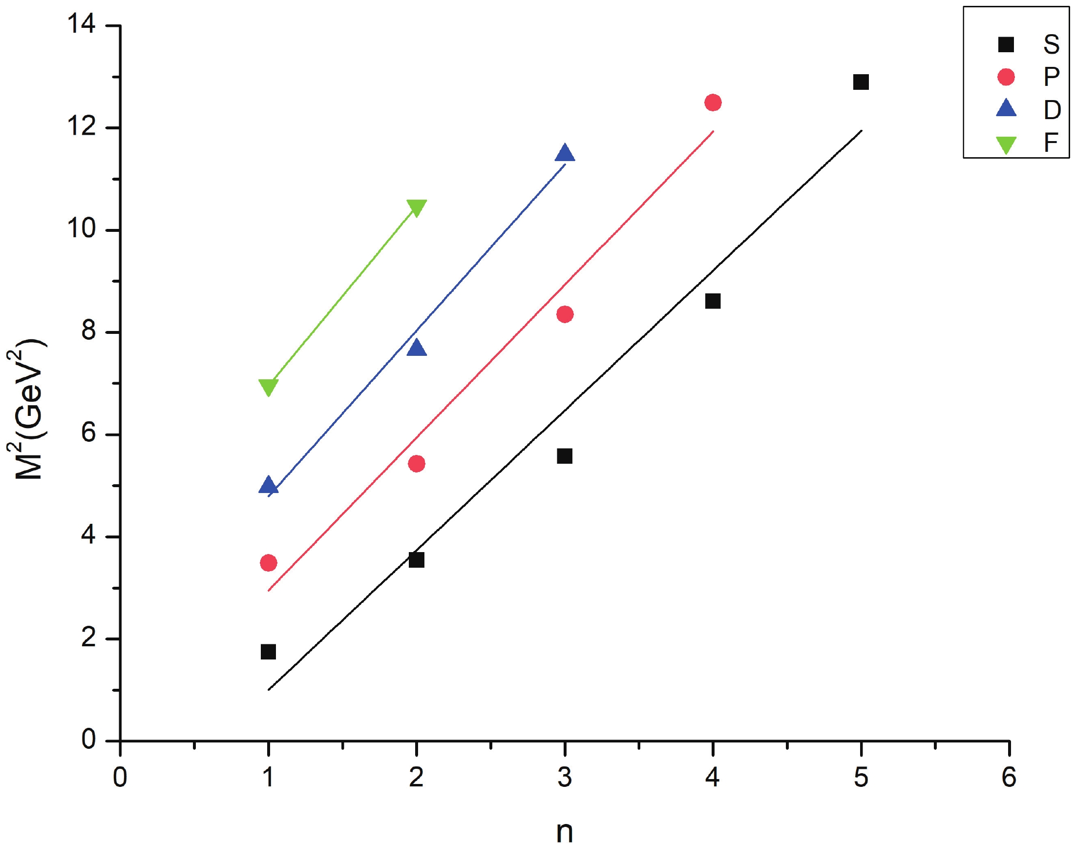 Figure1. (color online) Regge trajectory
 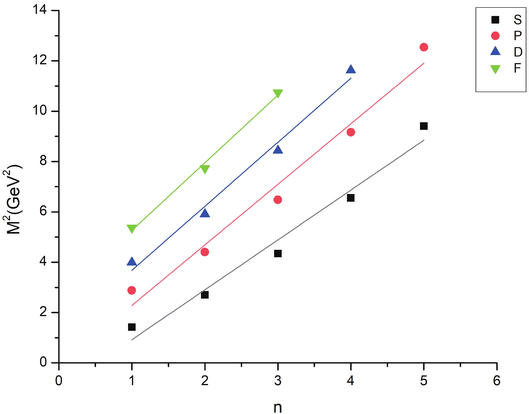 Figure2. (color online) Regge trajectory
 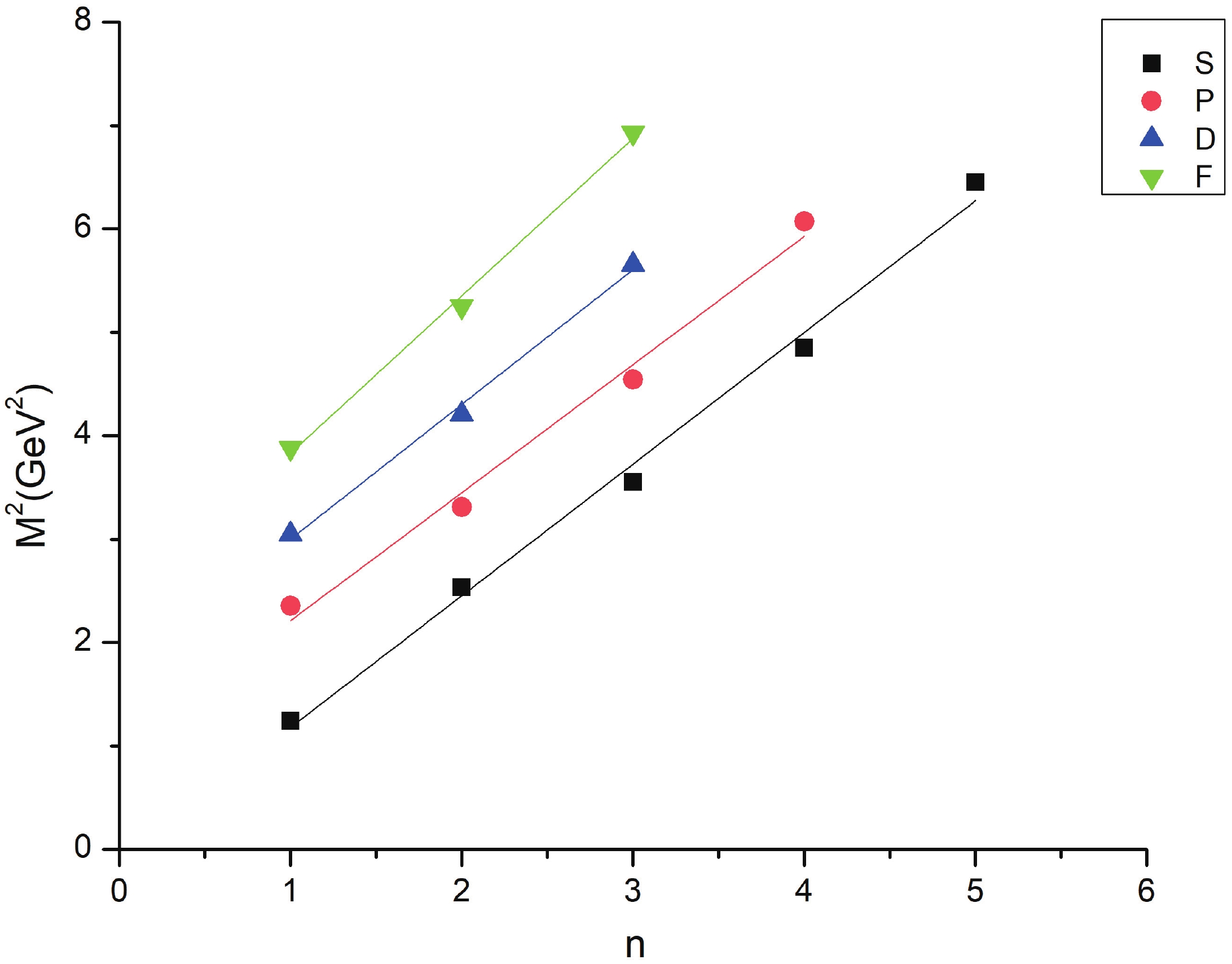 Figure3. (color online) Regge trajectory
 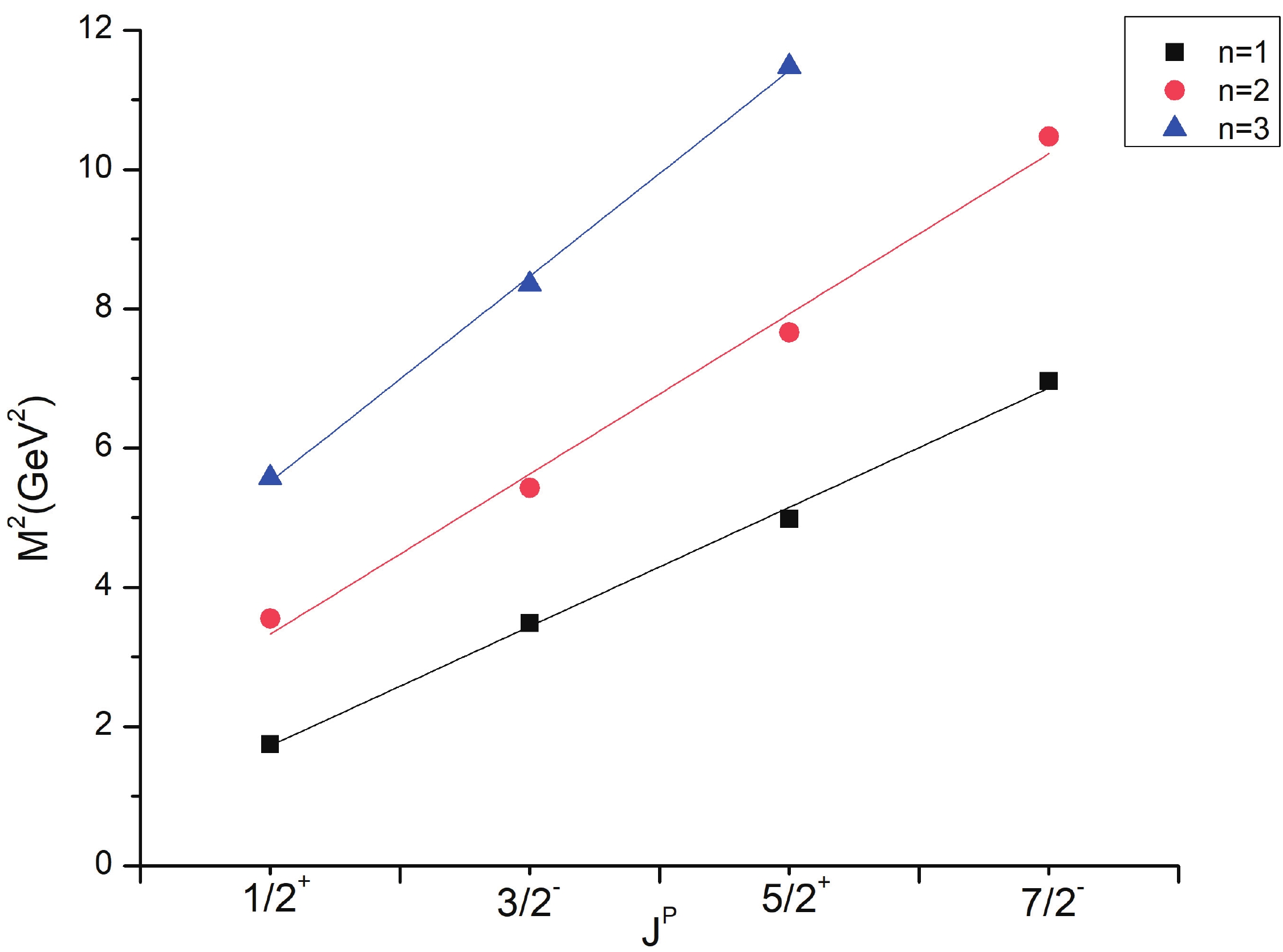 Figure4. (color online) Regge trajectory
 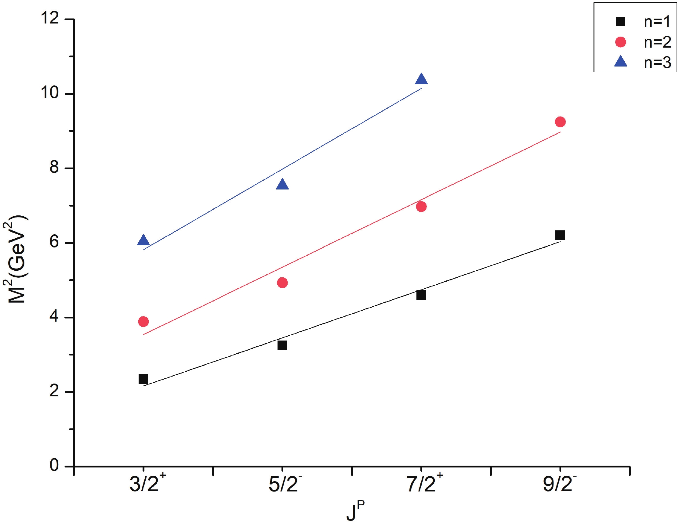 Figure5. (color online) Regge trajectory
 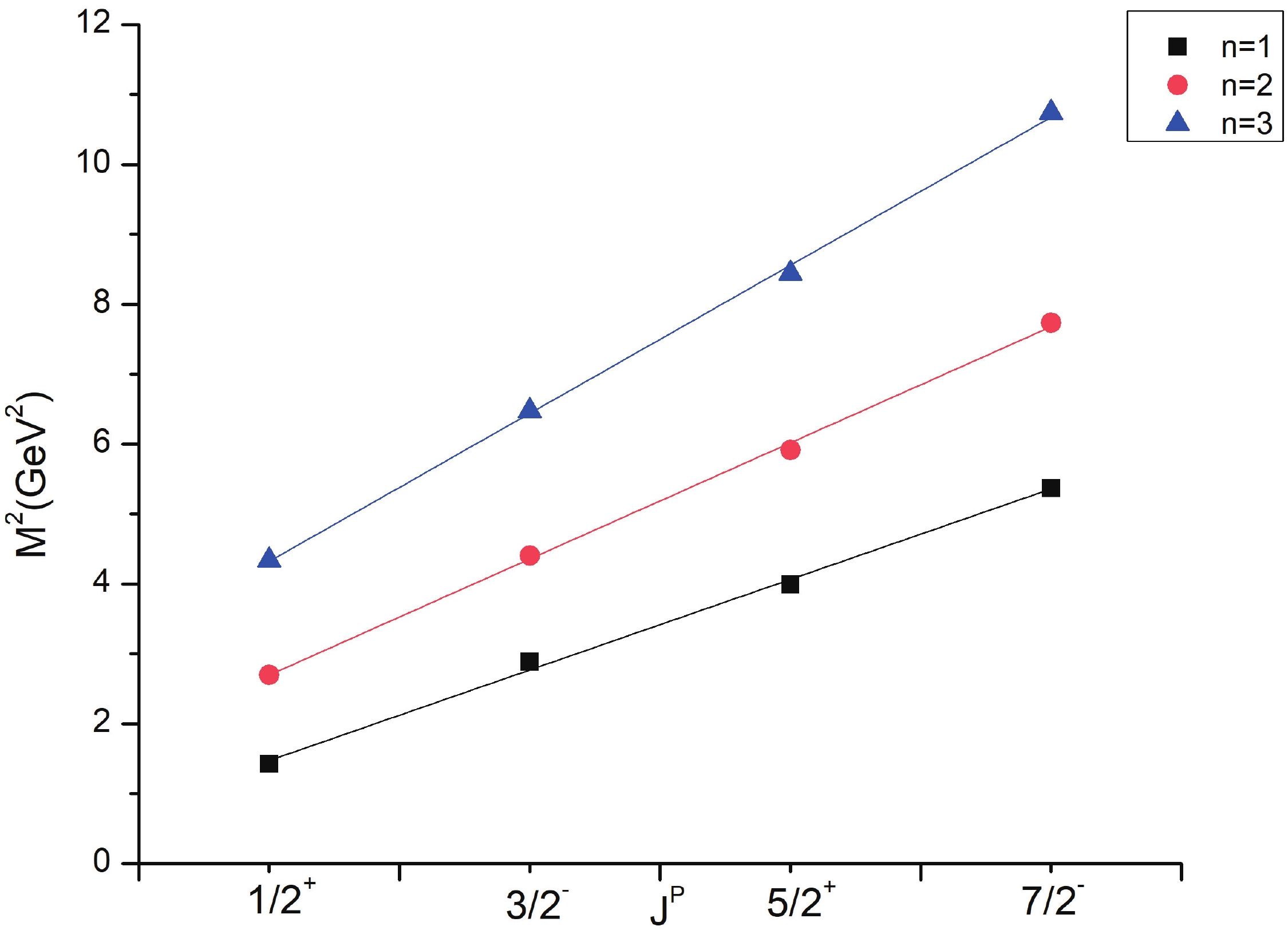 Figure6. (color online) Regge trajectory
 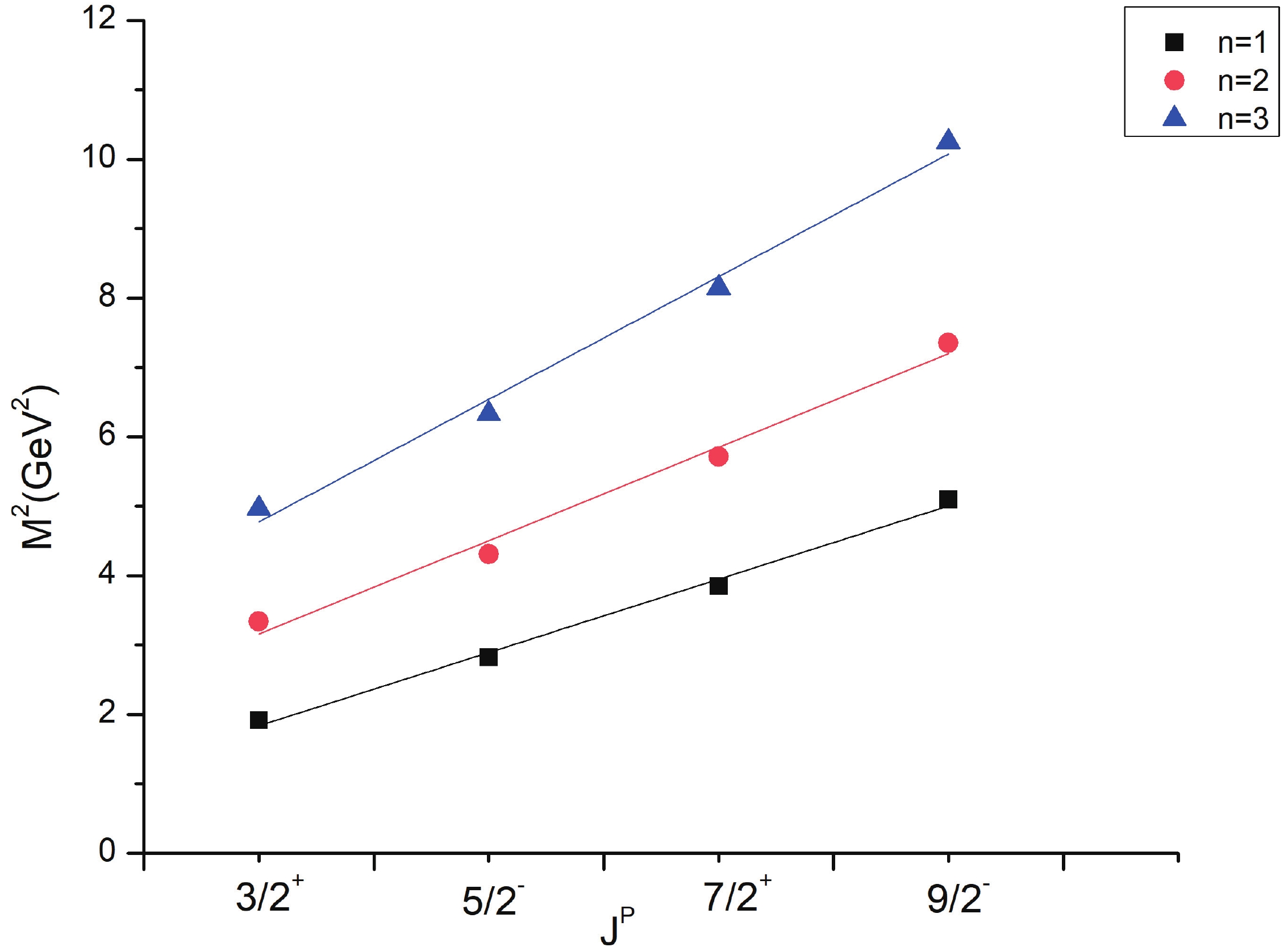 Figure7. (color online) Regge trajectory
 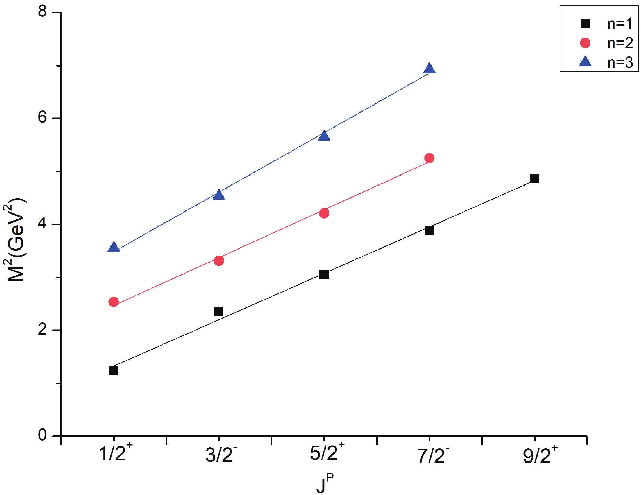 Figure8. (color online) Regge trajectory


