Ling Liu ^1,,
, Shuai Liu ^1,
, Shi-Sheng Zhang ^2,
, Li-Gang Cao ^3,4,,
,

Corresponding author: Ling Liu, liuling@synu.edu.cn

Corresponding author: Li-Gang Cao, caolg@bnu.edu.cn

1.College of Physics Science and Technology, Shenyang Normal University, Shenyang 110034, China
2.School of Physics, Beihang University, Beijing 100191, China
3.School of Mathematics and Physics, North China Electric Power University, Beijing 102206, China
4.Key Laboratory of Beam Technology of Ministry of Education, College of Nuclear Science and Technology, Beijing Normal University, Beijing 100875, China
Received Date:2020-07-11
Accepted Date:2020-12-02
Available Online:2021-04-15
Abstract:The isovector giant dipole resonances (IVGDR) in proton-rich Ar and Ca isotopes have been systematically investigated using the resonant continuum Hartree-Fock+BCS (HF+BCS) and quasiparticle random phase approximation (QRPA) methods. The Skyrme SLy5 and density-dependent contact pairing interactions are employed in the calculations. In addition to the giant dipole resonances at energy around 18 MeV, pygmy dipole resonances (PDR) are found to be located in the energy region below 12 MeV. The calculated energy-weighted moments of PDR in nuclei close to the proton drip-line exhaust about 4% of the TRK sum rule. The strengths decrease with increasing mass number in each isotopic chain. The transition densities of the PDR states show that motions of protons and neutrons are in phase in the interiors of nuclei, while the protons give the main contribution at the surface. By analyzing the QRPA amplitudes of proton and neutron 2-quasiparticle configurations for a given low-lying state, we find that only a few proton configurations give significant contributions. They contribute about 95% to the total QRPA amplitudes, which indicates that the collectivity of PDR states is not strong in proton-rich nuclei in the present study.

HTML

--> --> -->

Recently, the study of giant dipole resonances has been extended to unstable nuclei, as radioactive ion beam facilities have become available around the world. A new dipole excitation in the low energy region has been observed experimentally, called the pygmy dipole resonance (PDR). The PDR in neutron-rich nuclei is explained as a vibration in which the excess neutrons oscillate against a proton–neutron saturated core. The existence of the PDR in unstable nuclei may play a very important role in nuclear astrophysics because the PDR can affect the neutron-capture reaction cross sections contributing to nucleosynthesis and the abundance distribution of elements in the stars [1-3]. Moreover, a strong linear correlation between the PDR sum rule and the neutron skin has been found theoretically, which encourages constraints on the neutron skin and the density dependence of symmetry energy by the measured PDR strengths [4-8].
The PDR in neutron-rich nuclei has been studied extensively using different theoretical approaches, such as the deformed quasiparticle random phase approximation (QRPA) method based on Skyrme energy density functional theory [9], the relativistic QRPA [10], the relativistic quasiparticle time blocking approximation [11], the relativistic linear response theory [12-16], the relativistic deformed RPA [17], the shell model [18], the isospin-dependent quantum molecular dynamics model [19], and the RPA method with Gogny interaction [20]. Experimentally, the PDR in $ ^{20,22} $O, $ ^{26} $Ne, $ ^{68} $Ni, and $ ^{130,132} $Sn has been discovered and confirmed by different groups [21-24].
In proton-rich nuclei, a proton halo or skin is predicted in some cases [25-27]. The orbitals in the continuum play an important role in forming the halo structure [28-30]. Some proton halo or skin nuclei have been observed experimentally [31]. The study of proton-rich nuclei is also very important because they provide complementary insights to strong interactions, exhibit new forms of radioactivity, and are key for nucleosynthesis processes in astrophysics [32]. However, proton-rich nuclei have been found only for Z $ \leqslant $ 50 experimentally because of the Coulomb repulsive interaction. The proton drip line is much closer to the $ \beta $-stability line, and a proton halo or skin is possible only for the lighter isotopes. These reasons seem to disfavor the existence of a proton PDR in nuclei. No experimental observation of a proton PDR has been reported yet, and only a few theoretical studies have paid attention to the proton PDR using different models. The evolution of the low-lying E1 strength in proton-rich nuclei has been analyzed in the framework of relativistic QRPA [33-35]. In Ref. [36], the authors explored the PDR in proton-rich Ar isotopes using the unitary correlator operator method. The shell model has also been used to study the PDR in proton-rich nuclei [37]. A continuum random-phase approximation (CRPA) was used to investigate the PDR states in N = 20 isotones [38]. Recently, we applied the Skyrme HF+BCS plus QRPA to study the properties of the PDR in proton-rich $ ^{17,18} $Ne [39]. Knowledge of dipole excitations in nuclei towards the proton drip-line is rather limited. Measurement of the proton PDR should be possible in the near future at new facilities currently under construction, such as HIAF [40] in China.
In this work, we will explore the properties of dipole excitations of proton-rich Ar and Ca nuclei in a fully self-consistent approach. The ground states of these nuclei will be calculated within the Skyrme Hartree-Fock plus Bardeen-Cooper-Schrieffer (HF+BCS) approach, where the pairing correlations, including the contribution of resonant states in continuum, will be treated properly. The QRPA is then applied to obtain the excited dipole states of $ ^{32,34} $Ar and $ ^{34,36} $Ca. The properties of the PDR, including the excitation energies, energy (non-energy) weighted moments, transition densities, and collectivity, are analyzed in detail using our theoretical model.
The paper is organized as follows. The Skyrme HF+BCS and QRPA methods used in this work are briefly introduced in Section II. The properties of ground states and excited dipole states are presented and discussed in Section III. Finally, a summary and some remarks are given in Section IV.

The standard form of the Skyrme interaction and its energy density functional can be found in Ref. [41]. Within the Skyrme HF+BCS approximation, the quasiparticle wave functions and their quasiparticle energies are obtained from the self-consistent equation

$ \begin{array}{l} \left(- \nabla\dfrac{\hbar^2}{2m^*_b( r)} \cdot \nabla +U_b( r) \right)\psi_b( r) = \varepsilon_b\psi_b( r), \end{array} $

(1)

where $U_b( r) = V_c^b( r)+\delta_{b,\rm proton}V_{\rm coul}( r)-i V_{\rm so}^b( r)\cdot( \nabla\times \sigma) $, and $ V_c^b( r) $, $V_{\rm coul}( r)$, as well as $V_{\rm so}^b( r)$ are the nuclear central, coulomb, and spin-orbit fields, respectively.
Based on the calculated ground states, one can build the 2-quasiparticle (2${\rm qp}$) configurations for the QRPA calculations. Here, we will briefly summarize the formulas for the QRPA calculations. The well-known QRPA method [42] in matrix form is given by

$ \begin{array}{l} \left( \begin{array}{cc} A & B \\ B^* & A^* \end{array} \right) \left( \begin{array}{c} X^b \\ Y^b \end{array} \right) = E_b \left( \begin{array}{cc} 1 & 0\\ 0 & -1 \end{array} \right) \left( \begin{array}{c} X^b \\ Y^b \end{array} \right), \end{array} $

(2)

where $ E_b $ is the eigenvalue of the $ b $-th QRPA state and X$ ^b $, Y$ ^b $ are the corresponding forward and backward 2qp amplitudes, respectively.
The dipole strength in QRPA can be calculated as follows:

$ \begin{aligned}[b] B(EJ,E_b) =& \frac{1}{2J+1}\\&\times\left|\sum_{\mu\mu'}\left[X^b_{\mu\mu'} + Y^b_{\mu\mu'}\right] \langle \mu \|\hat{O}_J\| \mu' \rangle (u_\mu \nu_{\mu'}+ \nu_\mu u_{\mu'} )\right|^2, \end{aligned} $

(3)

where $ \nu $ and $ u $ are the occupation numbers of the quasiparticle levels.
The external field for isovector electric dipole excitation is defined as

$ \begin{aligned}[b] \hat{O}_{\mu}^{J = 1} = e\frac{N}{A}\sum_{i}^Z r_iY_{1\mu}(\hat{r}_i)-e\frac{Z}{A}\sum_{i}^N r_iY_{1\mu}(\hat{r}_i). \end{aligned} $

(4)

The discrete spectra are averaged with the Lorentzian distribution

$ \begin{aligned}[b] R(E) = \sum_{i} B(EJ,E_i)\frac{1}{\pi}\frac{\Gamma/2}{(E-E_i)^2+\Gamma^2/4}, \end{aligned} $

(5)

where the width of the Lorentz distribution is taken to be 0.5 MeV in the present calculations.
After solving the QRPA equation, various moments are defined as

$ \begin{aligned} m_k = \int E^kR(E) {\rm d} E. \end{aligned} $

(6)

2

-->

A.Ground-state properties of proton-rich Ar and Ca isotopes

First we will explore the ground state properties of proton-rich Ar and Ca isotopes. As pointed out in Refs. [43,44], the HF+BCS method is not well suited to describe nuclei close to the drip line because the continuum states in weakly bound nuclei are not correctly treated. Because of a nonzero occupation probability of quasibound states, there appears an unphysical gas of neutrons surrounding the nucleus [43,44]. The contribution of the coupling to the continuum would be prominent when the nucleus is close to the drip line, therefore a proper treatment of the continuum becomes more important. To do so, one can perform the calculations with the non-relativistic Hartree-Fock-Bogoliubov (HFB) [43,44] or relativistic Hartree-Bogoliubov (RHB) [45] method. On the other hand, it has also been pointed out that pairing correlations could be described well by the simple HF+BCS theory if single-particle states in the continuum are properly treated [46-49]. This method is called the resonant continuum HF+BCS (HF+BCSR) approximation. It has been shown [50] that the resonant continuum HF+BCS approximation could reproduce the pairing correlation energies predicted by the continuum HFB approach up to the drip line.
To investigate the ground state properties of proton-rich Ar and Ca isotopes, we have extended the Skyrme HF+BCS method of Eq. (1) to the resonant continuum Skyrme HF+BCS by properly including the contribution of continuum resonant states. The equations are solved in coordinate space. We introduce single-particle resonant states into the pairing gap equations instead of the discretized continuous states. The wave functions of resonant states are obtained by imposing a scattering boundary condition [51]. More details of the resonant continuum HF+BCS method are given in Refs. [46-50].
In the present study, a spherical shape is assumed for proton-rich nuclei. The Skyrme interaction SLy5 is adopted [41]. For the pairing correlations, we adopt a mixed type density-dependent contact pairing interaction in our calculations [52]. The strength V₀ is adjusted to reproduce the neutron or proton gaps in $ ^{34} $Ar and $ ^{36} $Ca. For the neutron and proton pairing in $ ^{34} $Ar, V₀ is 560.9 MeVfm$ ^3 $ and 619.1 MeVfm$ ^3 $, respectively. It is 566.2 MeVfm$ ^3 $ for the neutron pairing in $ ^{36} $Ca. For the pairing window, we choose the states up to 1$ f_{7/2} $ for proton-rich Ar and Ca isotopes. The single-particle resonant states in the continuum are investigated in terms of the S-matrix method. The resonant state is characterized by the phase shift crossing $ \pi/2 $, where the scattering cross section of the corresponding partial wave reaches its maximum. The width of a resonant state is the full width at half maximum (FWHM) for the corresponding partial wave scattering cross section. The energies and widths of the calculated single-particle resonances for proton-rich Ar and Ca are listed in Table 1. Although the neutron resonant states 1$ f_{5/2} $ and 1$ g_{9/2} $ are not included in the pairing window, we also put the calculated results in Table 1. Due to the sufficiently high centrifugal barrier and Coulomb barrier, the widths of the proton resonant states 1$ d_{3/2} $ and 1$ f_{7/2} $ are rather narrow, especially for 1$ d_{3/2} $ in $ ^{30} $Ar and $ ^{32} $Ca, as well as 1$ f_{7/2} $ in $ ^{32,34} $Ar and $ ^{34,36} $Ca. These states are rather stable and have bound state characteristics. As an example, the single-particle levels for $ ^{30} $Ar and $ ^{32} $Ca are shown in Fig. 1 together with the central potentials. The states with positive energy in the continuum in Fig. 1 are the resonant states we have found. We plot the proton densities of $ ^{30} $Ar and $ ^{32} $Ca in Fig. 2, where the solid, short-dashed, and short-dotted curves are obtained in the HF+BCS approximation by choosing the box size as 16, 20, and 24 fm, respectively, and the short dash-dotted curves are produced in the HF+BCSR approximation. It is observed that the tail of the density depends on the box size in the HF+BCS approximation, and an unphysical particle gas may appear in exotic nuclei, whereas the behaviours of proton densities are rather stable when one performs the resonant continuum HF+BCS calculations.

Nucleus	proton			neutron		Nucleus	proton			neutron
	state	E$_p$		state	E$_n$		state	E$_p$		state	E$_n$
$^{30}$Ar	1d$_{3/2}$	0.202+i0.000		1f$_{5/2}$	0.010+i0.000	$^{32}$Ca	1d$_{3/2}$	0.489+i0.000		1g$_{9/2}$	2.455+i0.026
	1f$_{7/2}$	5.226+i0.166		1g$_{9/2}$	4.544+i0.249		1f$_{7/2}$	5.158+i0.123
$^{32}$Ar	1f$_{7/2}$	3.097+i0.009		1f$_{5/2}$	0.448+i0.001	$^{34}$Ca	1f$_{7/2}$	3.088+i0.006		1g$_{9/2}$	2.764+i0.040
				1g$_{9/2}$	4.825+i0.305
$^{34}$Ar	1f$_{7/2}$	0.983+i0.000		1f$_{5/2}$	0.584+i0.003	$^{36}$Ca	1f$_{7/2}$	1.044+i0.000		1g$_{9/2}$	2.779+i0.042
				1g$_{9/2}$	4.741+i0.293

Table1.Energies and widths of single-particle resonant states in proton-rich Ar and Ca isotopes. The results are calculated with the SLy5 parameter set. All energies are in MeV.

Figure1. Proton and neutron single-particle levels for $ ^{30} $Ar (a) and $ ^{32} $Ca (b). All results are obtained in the Skyrme HF+BCSR calculations with the SLy5 parameter set.

Figure2. (color online) Proton density distributions in proton-rich nuclei $ ^{30} $Ar (a) and $ ^{32} $Ca (b). The results are obtained in the Skyrme HF+BCS and HF+BCSR approximation with the SLy5 parameter set.

In Table 2 we show the calculated ground state properties for proton-rich Ar and Ca isotopes with the Skyrme HF+BCSR approximation, including the total binding energies, one-proton and two-proton separation energies, neutron and proton Fermi energies, root-mean-square radii (rms radii), and charge radii. Values in parentheses are the corresponding experimental data from Refs. [53,54]. It is found that the predicted total binding energies for most of the nuclei are about 3-5 MeV larger than the experimental data. We have checked that similar results are obtained by using other Skyrme interactions. The one-proton and two-proton separation energies provide information on whether a nucleus is stable against one or two proton emissions, and thus define the proton drip lines. One can see from the table that the calculated separation energies of $ ^{30} $Ar and $ ^{32} $Ca become negative, which means that these two nuclei are unbound and stay at the proton drip line, so we will not include these two nuclei in the IVGDR calculations below. The Fermi energies of the proton-rich Ca nuclei in Table 2 are obtained simply by using the average value of the energies of the last hole state and first particle state. They are not calculated using the BCS approximation because proton number 20 is a magic number. The Fermi energies of protons change from negative to positive as the nuclei become more and more proton-rich. As we can see from Table 2, the calculated proton Fermi energies of $ ^{30} $Ar and $ ^{32} $Ca are positive, which again means these two nuclei are unbound and proton decay may occur. Although the proton Fermi energy obtained with the simple approach in $ ^{34} $Ca is positive, the energy of the last occupied proton level is -1.48 MeV, indicating that this nucleus is weakly bound. The neutron and proton density distributions in $ ^{32,34} $Ar and $ ^{34,36} $Ca are displayed in Fig. 3. It is clearly seen that the proton density distributions are much extended outside compared to those of neutrons. The predicted proton rms radii are much larger than those of neutrons, which suggests that a proton skin could be formed in these nuclei. The experimental charge radii of $ ^{32,34} $Ar are reproduced well by our theoretical model.

	$E_B$	S$_p$	S$_{2p}$	$\lambda_n$	$\lambda_p$	$r_n$	$r_p$	$r_c$
$^{30}$Ar	213.2	?0.15	?2.10	?19.79	0.28	3.017	3.344	3.437
$^{32}$Ar	249.9(246.4)	2.76	2.58	?17.39	?1.87	3.092	3.315	3.409(3.346)
$^{34}$Ar	281.4(278.7)	5.63	7.29	?14.86	?4.18	3.188	3.313	3.407(3.365)
$^{32}$Ca	209.9	?1.44	?3.32	?21.82	1.49	3.060	3.459	3.550
$^{34}$Ca	250.1(244.9)	0.42	0.12	?19.53	0.51	3.134	3.410	3.502
$^{36}$Ca	285.4(281.4)	2.86	4.06	?17.13	?1.30	3.222	3.401	3.493

Table2.The calculated ground state properties of proton-rich Ar and Ca nuclei, including the total binding energies ($E_B$), one-proton separation energies (S$_p$) and two-proton separation energies (S$_{2p}$), neutron and proton Fermi energies ($\lambda_n$,$\lambda_p$), neutron and proton rms radii ($r_n$,$r_p$) and charge radii ($r_c$). Values in parentheses are the corresponding experimental data [53,54]. Energies are in MeV and radii are in fm.

Figure3. (color online) Neutron and proton density distributions in proton-rich $ ^{32,34} $Ar and $ ^{34,36} $Ca nuclei. All results are obtained in the Skyrme HF+BCSR approximation with the SLy5 parameter set.

2 -->

B.Properties of 1$ ^- $ excited states in proton-rich Ar and Ca isotopes

To obtain the dipole excitations of proton-rich Ar and Ca nuclei, we have performed the fully self-consistent QRPA calculations by using the SLy5 Skyrme interaction. There is no approximation in the residual interaction, since all its terms are considered the same as that used in the ground state calculations. The details of the residual interaction can be found in Ref. [55]. After solving the HF+BCS equations in coordinate space, we build up a model space of two-quasiparticle configurations for dipole excitation, and then solve the QRPA matrix equation in that space. The $ \Delta_n = 12 $ shell cut-off is adopted to build up the QRPA model space, which is large enough that the isovector dipole energy-weighted moment exhausts practically 99.9% of the double-commutator (DC) value. Since we discretize the continuum by using the box approximation, the QRPA results may depend on the box size. In Table 3, we show the calculated total QRPA E1 strengths, energy-weighted moments and centroid energies in the energy region 0 $ < E \leqslant $40 MeV for $ ^{32} $Ar, calculated by setting the box size as 16, 20, 24 and 28 fm, respectively. The results in lower (0 $ \leqslant $ E $ \leqslant $ 12 MeV) and higher (12 $ < $ E $ \leqslant $ 40 MeV) energy regions are also presented. The strength distributions are plotted in Fig. 4. As we know, the properties of the ground state are calculated with the HF+BCSR method, and are independent of the box size since the widths of resonant states in the continuum are rather narrow, and their energies are stable when using different box sizes. For the other states in the continuum used to build the QRPA quasiparticle configurations, like the nonresonant states, these states are obtained by discretizing the continuum with the box approximation, and their eigenvalues and wavefunctions keep changing with increasing box size. The changes may affect the calculated properties of dipole states, as shown in Fig. 4; the distributions of the calculated strengths are slightly different, and the seesaw structure of the states around 12 MeV may affect the values of the lower and higher energy regions shown in Table 3. Anyway, better converged results are obtained if we use a box size larger than 20 fm. For example, the calculated energy-weighted moment in 0 $ < E \leqslant $40 MeV for R = 24 fm is 129.71 e$ ^2 $fm$ ^2 $MeV, and the DC value is 130.95 e$ ^2 $fm$ ^2 $MeV, which exhausts about 99.1% of the DC value. So all results are calculated by setting the box size as 24 fm in this study.

R/fm	0 $< E \leqslant$40 MeV				0 $ < E \leqslant$12 MeV				12 $< E \leqslant$40 MeV
	$m_{0}$	$m_{1}$	$E_c$		$m_{0}$	$m_{1}$	$E_c$		$m_{0}$	$m_{1}$	$E_c$
16	6.996	128.510	18.34		0.369	3.628	9.83		6.627	124.882	18.85
20	6.992	128.391	18.36		0.447	4.580	10.26		6.545	123.811	18.92
24	7.038	129.709	18.43		0.333	3.204	9.63		6.705	126.505	18.87
28	6.942	127.783	18.41		0.356	3.331	9.36		6.586	124.452	18.90

Table3.Total QRPA E1 strengths $m_{0}$ (in e$^2$fm$^2$), energy-weighted moments $m_{1}$(in e$^2$fm$^2$MeV) and centroid energies $E_c$ (in MeV) in the energy region 0 $< E \leqslant$40 MeV for $^{32}$Ar, calculated by setting the box size as 16, 20, 24 and 28 fm, respectively. The values for lower (0 $ < E \leqslant$12 MeV) and higher (12 $ < E \leqslant$40 MeV) energy regions are also presented.

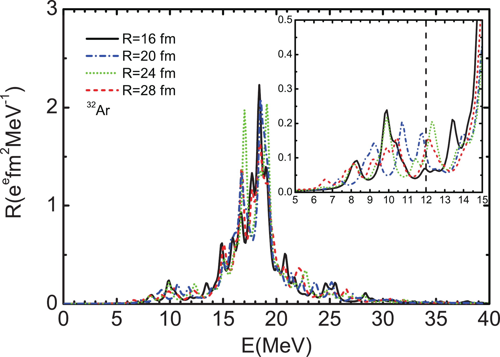Figure4. (color online) The QRPA strength distributions of $ ^{32} $Ar calculated with different box size R. The low-lying strengths between 5 and 15 MeV are also displayed in the insert. The width of the Lorentz distribution is set to be 0.5 MeV.

In Fig. 5 we show the calculated dipole strength distributions of proton-rich Ar and Ca nuclei, denoted by solid lines. The discrete QRPA peaks have been smeared out by using a Lorentzian function. Pronounced peaks located at energy around 18 MeV for proton-rich Ar and Ca nuclei are found, which correspond to the normal GDR strengths. In the energy region below 12 MeV, there are some low-lying strengths which appear for all selected proton-rich nuclei. For $ ^{32} $Ar and $ ^{34} $Ca nuclei, the low-lying strengths are more notable. They are the so-called PDR strengths which appear in unstable nuclei.
Figure5. The QRPA strength distributions of proton-rich Ar (a,b) and Ca (c,d) nuclei for isovector dipole excitation. The width of the Lorentz distribution is set to be 0.5 MeV.

In Table 4 we show the energy (non-energy)-weighted moment $ m_1 $ ($ m_0 $) and the centroid energies of dipole strengths of Ar and Ca nuclei calculated in the QRPA. We separate the energy region into two parts: the lower energy part (0 MeV $ < E \leqslant $ 12 MeV) and the higher energy part (12 MeV $ < E \leqslant $ 40 MeV), where the PDR and GDR strengths are mainly distributed. The classical TRK dipole sum rules for those nuclei are also given in the table. It is clearly seen that the values of energy (non-energy)-weighted moment $ m_1 $ ($ m_0 $) of PDR states decrease in each isotopic chain as the mass numbers of nuclei increase. For example, the energy (non-energy)-weighted moment $ m_1 $ ($ m_0 $) of PDR states in $ ^{32} $Ar is 3.204 e$ ^2 $fm$ ^2 $MeV (0.333 e$ ^2 $fm$ ^2 $), while the value in $ ^{34} $Ar is about 2.971 e$ ^2 $fm$ ^2 $MeV (0.274 e$ ^2 $fm$ ^2 $). The energy-weighted moments $ m_1 $ of PDR states in these nuclei exhaust about 2 to 4 percent of the TRK sum rule. For the nucleus $ ^{32} $Ar ($ ^{34} $Ca), it is about 3% (4%). For the GDR states, the energy (non-energy)-weighted moment $ m_1 $ ($ m_0 $) increases in each isotopic chain as the mass numbers increase. The energy weighted moments for all selected nuclei exhaust about 107% of the TRK sum rule. The calculated centroid energies of the GDR are distributed at an energy around 18.5 MeV for all nuclei; the energy is smaller for the heavier nucleus in each isotopic chain. For the PDR, the energies are around 10.0 MeV; it is larger for the heavier nucleus in each isotopic chain.

	0$ < E \leqslant$12				12$< E \leqslant$40			S$_{\text{TRK}}$
	$m_{0}$	$m_{1}$	$E_c$		$m_{0}$	$m_{1}$	$E_c$
$^{32}$Ar	0.333	3.204	9.63		6.705	126.51	18.87	117.33
$^{34}$Ar	0.274	2.971	10.82		7.261	135.49	18.66	126.21
$^{34}$Ca	0.548	4.783	8.73		6.976	128.60	18.43	122.71
$^{36}$Ca	0.302	2.769	9.18		7.757	141.45	18.24	132.44

Table4.The energy (non-energy)-weighted moments $m_1$ ($m_0$) and the centroid energies of dipole strengths in lower and higher energy regions. The values in the last column are obtained from the classical TRK dipole sum rule (e$^2$fm$^2$MeV). The units are e$^2$fm$^2$ and e$^2$fm$^2$MeV for $m_0$ and $m_1$, respectively. Energies are in MeV.

The calculated proton and neutron transition densities of the PDR states (marked with energies less or around 12 MeV) and GDR states (marked with energies larger than 15 MeV) are shown in Fig. 6 (for Ar isotopes) and Fig. 7 (for Ca isotopes). For the PDR states we can see from the figures that the protons and neutrons move in phase in the nuclear interior, while the contribution at the surface comes mainly from protons. This shows that the low-lying states in proton-rich nuclei are typical pygmy resonances, similar to what has been found in neutron-rich nuclei. The nature of the PDR states in neutron-rich nuclei has been discussed extensively in several publications [56-59]. For the nature of PDR states in proton-rich nuclei, one may need to analyze the properties of isoscalar dipole resonances as done in Refs. [56-59]. This needs more work and is not discussed further in the present study. The transition densities for the GDR states show that the motions of protons and neutrons are out of phase, and there is almost no contribution from either protons or neutrons in the exterior region, which is the typical isovector GDR mode.
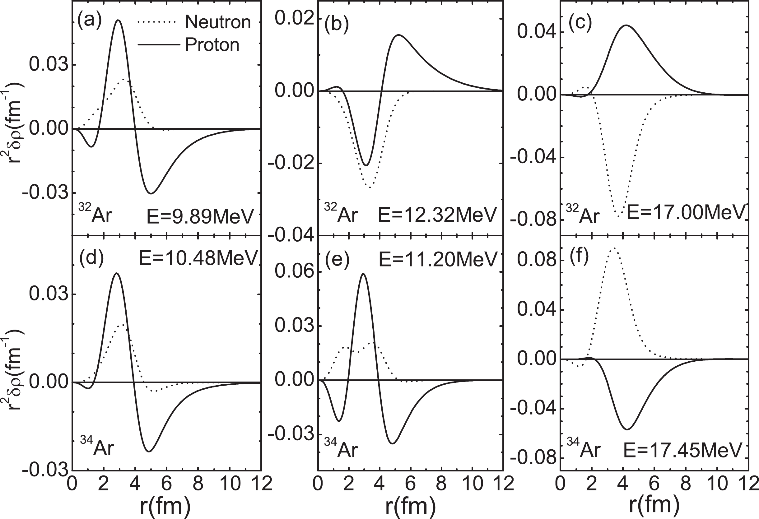Figure6. Calculated proton and neutron transition densities for the PDR states and GDR states in proton-rich $ ^{32,34} $Ar. The SLy5 effective interaction is employed in the calculations.

Figure7. Same as in Fig. 6. Calculated proton and neutron transition densities for the PDR states and GDR states in proton-rich $ ^{34,36} $Ca. The SLy5 effective interaction is employed in the calculations.

The QRPA amplitudes of proton and neutron 2qp configuration for a given excited state b are expressed as

$ \begin{array}{l} \xi^b_{2qp} = |X^b_{2qp}|^2-|Y^b_{2qp}|^2 \end{array} $

(7)

and the normalization condition

$ \begin{array}{l} \sum_{2qp}\xi^b_{2qp} = 1. \end{array} $

(8)

In Table 5 we show the largest QRPA amplitudes of proton and neutron 2qp configurations for the given excited states in the proton-rich Ar and Ca nuclei, which can help us in understanding the collectivity of dipole states. For GDR states, as we can see, there are more than 10 2qp configurations with amplitude larger than 1%, which means a coherent superposition of many 2qp configurations and shows the collective excitation of the GDR states. For the PDR states, however, only a few configurations give a significant contribution. For proton-rich Ar nuclei, the proton configurations ($ 3p_{3/2}2s_{1/2}^{-1})^\pi $, ($ 4p_{1/2}1d_{3/2}^{-1})^\pi $ and ($ 3p_{1/2}1d_{3/2}^{-1})^\pi $ contribute more than 86% to the total QRPA amplitude for the first PDR state, as shown in Table 5. For the second PDR states in Table 5, the main contribution to the total QRPA amplitude is from protons in $ 2s_{1/2} $ and $ 1d_{3/2} $ orbitals, which contribute more than 90% to the total QRPA amplitude. For the PDR in proton-rich Ca nuclei, the proton 2qp configurations ($ 3p_{3/2}2s_{1/2}^{-1})^\pi $, ($ 3f_{5/2}1d_{3/2}^{-1})^\pi $ and $ (4p_{\frac{1}{2}}2s_{\frac{1}{2}}^{-1})^\pi $ dominate in the QRPA amplitudes. For example, in $ ^{34} $Ca and $ ^{36} $Ca, the proton 2qp configuration ($ 3p_{3/2}2s_{1/2}^{-1})^\pi $ contributes about 83% to the total QRPA amplitude for the first 1$ ^- $ state at energies E = 9.38 MeV and E = 10.55 MeV, respectively. For the second notable PDR states shown in Table 5, the main contribution also comes mainly from the protons in $ 2s_{1/2} $ and $ 1d_{3/2} $ orbitals, as for the Ar isotopes, and they contribute more than 99% to the total QRPA amplitude. All those results show that the PDR states in proton-rich Ar and Ca nuclei are more like a quasiparticle excitation. In Ref. [60], the authors studied the evolution of collectivity in the isovector dipole response in the low-energy region of neutron-rich isotopes of O, Ca, Ni, Zr, and Sn. They found that the onset of dipole strength in the low-energy region is due to single-particle excitations of the loosely bound neutrons in light nuclei. Our results are similar to what was found by the authors of Ref. [60].

$ ^{32} $Ar							$ ^{34} $Ar
E = 9.89 MeV	$ \xi^b_{2qp} $	E = 12.32 MeV	$ \xi^b_{2qp} $	E = 17.00 MeV	$ \xi^b_{2qp} $		E = 10.49 MeV	$ \xi^b_{2qp} $	E = 11.20 MeV	$ \xi^b_{2qp} $	E = 17.45 MeV	$ \xi^b_{2qp} $
$ (1f_{\frac{7}{2}}1d_{\frac{5}{2}}^{-1})^\pi $	3%	$ (4p_{\frac{1}{2}}2s_{\frac{1}{2}}^{-1})^\pi $	5%	$ (1d_{\frac{3}{2}}1p_{\frac{1}{2}}^{-1})^\pi $	4%		$ (1f_{\frac{7}{2}}1d_{\frac{5}{2}}^{-1})^\pi $	2%	$ (1f_{\frac{7}{2}}1d_{\frac{5}{2}}^{-1})^\pi $	6%	$ (1f_{\frac{7}{2}}1d_{\frac{5}{2}}^{-1})^\pi $	13%
$ (3p_{\frac{3}{2}}2s_{\frac{1}{2}}^{-1})^\pi $	28%	$ (5p_{\frac{1}{2}}1d_{\frac{3}{2}}^{-1})^\pi $	7%	$ (1f_{\frac{7}{2}}1d_{\frac{5}{2}}^{-1})^\pi $	20%		$ (2p_{\frac{3}{2}}2s_{\frac{1}{2}}^{-1})^\pi $	2%	$ (3p_{\frac{1}{2}}2s_{\frac{1}{2}}^{-1})^\pi $	1%	$ (4p_{\frac{3}{2}}1d_{\frac{5}{2}}^{-1})^\pi $	9%
$ (4p_{\frac{1}{2}}1d_{\frac{3}{2}}^{-1})^\pi $	58%	$ (5p_{\frac{3}{2}}1d_{\frac{3}{2}}^{-1})^\pi $	21%	$ (5p_{\frac{3}{2}}1d_{\frac{5}{2}}^{-1})^\pi $	9%		$ (3p_{\frac{3}{2}}2s_{\frac{1}{2}}^{-1})^\pi $	3%	$ (3p_{\frac{3}{2}}2s_{\frac{1}{2}}^{-1})^\pi $	68%	$ (3f_{\frac{7}{2}}1d_{\frac{5}{2}}^{-1})^\pi $	12%
$ (4p_{\frac{3}{2}}1d_{\frac{3}{2}}^{-1})^\pi $	6%	$ (3f_{\frac{5}{2}}1d_{\frac{3}{2}}^{-1})^\pi $	62%	$ (4f_{\frac{7}{2}}1d_{\frac{5}{2}}^{-1})^\pi $	3%		$ (3p_{\frac{1}{2}}1d_{\frac{3}{2}}^{-1})^\pi $	86%	$ (3p_{\frac{1}{2}}1d_{\frac{3}{2}}^{-1})^\pi $	7%	$ (5p_{\frac{3}{2}}2s_{\frac{1}{2}}^{-1})^\pi $	3%
$ (2d_{\frac{5}{2}}1f_{\frac{7}{2}}^{-1})^\pi $	1%	$ (1f_{\frac{7}{2}}1d_{\frac{5}{2}}^{-1})^\pi $	1%	$ (6p_{\frac{3}{2}}2s_{\frac{1}{2}}^{-1})^\pi $	7%		$ (3p_{\frac{3}{2}}1d_{\frac{3}{2}}^{-1})^\pi $	5%	$ (4p_{\frac{1}{2}}1d_{\frac{3}{2}}^{-1})^\pi $	5%	$ (6p_{\frac{3}{2}}2s_{\frac{1}{2}}^{-1})^\pi $	2%
				$ (6p_{\frac{1}{2}}1d_{\frac{3}{2}}^{-1})^\pi $	18%				$ (4p_{\frac{3}{2}}1d_{\frac{3}{2}}^{-1})^\pi $	9%	$ (6p_{\frac{1}{2}}1d_{\frac{3}{2}}^{-1})^\pi $	2%
				$ (5f_{\frac{5}{2}}1d_{\frac{3}{2}}^{-1})^\pi $	5%						$ (6p_{\frac{3}{2}}1d_{\frac{3}{2}}^{-1})^\pi $	2%
				$ (1f_{\frac{7}{2}}1d_{\frac{5}{2}}^{-1})^\nu $	4%						$ (2s_{\frac{1}{2}}1p_{\frac{1}{2}}^{-1})^\nu $	23%
				$ (2p_{\frac{3}{2}}1d_{\frac{5}{2}}^{-1})^\nu $	6%						$ (1f_{\frac{7}{2}}1d_{\frac{5}{2}}^{-1})^\nu $	14%
				$ (2p_{\frac{1}{2}}2s_{\frac{1}{2}}^{-1})^\nu $	3%						$ (2p_{\frac{3}{2}}1d_{\frac{5}{2}}^{-1})^\nu $	3%
$ ^{34} $Ca							$ ^{36} $Ca
E = 9.38 MeV	$ \xi^b_{2qp} $	E = 10.28 MeV	$ \xi^b_{2qp} $	E = 16.48 MeV	$ \xi^b_{2qp} $		E = 10.55 MeV	$ \xi^b_{2qp} $	E = 12.54 MeV	$ \xi^b_{2qp} $	E = 18.03 MeV	$ \xi^b_{2qp} $
$ (1f_{\frac{7}{2}}1d_{\frac{5}{2}}^{-1})^\pi $	2%	$ (4p_{\frac{1}{2}}2s_{\frac{1}{2}}^{-1})^\pi $	2%	$ (1f_{\frac{7}{2}}1d_{\frac{5}{2}}^{-1})^\pi $	7%		$ (1f_{\frac{7}{2}}1d_{\frac{5}{2}}^{-1})^\pi $	4%	$ (4p_{\frac{1}{2}}2s_{\frac{1}{2}}^{-1})^\pi $	70%	$ (4p_{\frac{3}{2}}1d_{\frac{5}{2}}^{-1})^\pi $	2%
$ (3p_{\frac{1}{2}}2s_{\frac{1}{2}}^{-1})^\pi $	5%	$ (4p_{\frac{3}{2}}2s_{\frac{1}{2}}^{-1})^\pi $	2%	$ (6p_{\frac{1}{2}}2s_{\frac{1}{2}}^{-1})^\pi $	4%		$ (3p_{\frac{1}{2}}2s_{\frac{1}{2}}^{-1})^\pi $	2%	$ (3f_{\frac{5}{2}}1d_{\frac{3}{2}}^{-1})^\pi $	15%	$ (5p_{\frac{3}{2}}1d_{\frac{5}{2}}^{-1})^\pi $	3%
$ (3p_{\frac{3}{2}}2s_{\frac{1}{2}}^{-1})^\pi $	87%	$ (3f_{\frac{5}{2}}1d_{\frac{3}{2}}^{-1})^\pi $	90%	$ (6p_{\frac{3}{2}}2s_{\frac{1}{2}}^{-1})^\pi $	10%		$ (3p_{\frac{3}{2}}2s_{\frac{1}{2}}^{-1})^\pi $	83%	$ (4f_{\frac{5}{2}}1d_{\frac{3}{2}}^{-1})^\pi $	8%	$ (1f_{\frac{7}{2}}1d_{\frac{5}{2}}^{-1})^\pi $	3%
$ (5p_{\frac{3}{2}}1d_{\frac{3}{2}}^{-1})^\pi $	1%	$ (4f_{\frac{5}{2}}1d_{\frac{3}{2}}^{-1})^\pi $	2%	$ (5f_{\frac{5}{2}}1d_{\frac{3}{2}}^{-1})^\pi $	5%		$ (4p_{\frac{1}{2}}1d_{\frac{3}{2}}^{-1})^\pi $	4%	$ (3p_{\frac{3}{2}}1d_{\frac{5}{2}}^{-1})^\pi $	1%	$ (6p_{\frac{1}{2}}2s_{\frac{1}{2}}^{-1})^\pi $	3%
				$ (1d_{\frac{5}{2}}1p_{\frac{3}{2}}^{-1})^\nu $	7%		$ (5p_{\frac{1}{2}}1d_{\frac{3}{2}}^{-1})^\pi $	1%	$ (2p_{\frac{3}{2}}2s_{\frac{1}{2}}^{-1})^\nu $	2%	$ (6p_{\frac{3}{2}}2s_{\frac{1}{2}}^{-1})^\pi $	3%
				$ (2s_{\frac{1}{2}}1p_{\frac{1}{2}}^{-1})^\nu $	18%						$ (5f_{\frac{5}{2}}1d_{\frac{3}{2}}^{-1})^\pi $	30%
				$ (1d_{\frac{3}{2}}1p_{\frac{1}{2}}^{-1})^\nu $	2%						$ (2s_{\frac{1}{2}}1p_{\frac{1}{2}}^{-1})^\nu $	4%
				$ (1f_{\frac{7}{2}}1d_{\frac{5}{2}}^{-1})^\nu $	24%						$ (1d_{\frac{3}{2}}1p_{\frac{1}{2}}^{-1})^\nu $	18%
				$ (2p_{\frac{1}{2}}2s_{\frac{1}{2}}^{-1})^\nu $	4%						$ (2p_{\frac{3}{2}}1d_{\frac{5}{2}}^{-1})^\nu $	15%
				$ (2p_{\frac{3}{2}}2s_{\frac{1}{2}}^{-1})^\nu $	3%						$ (2p_{\frac{1}{2}}2s_{\frac{1}{2}}^{-1})^\nu $	2%

Table5.The largest contributions of the proton and neutron 2qp excitations to the isovector reduced dipole QRPA amplitudes for the given states for proton-rich Ar and Ca nuclei.

In conclusion, we have systematically studied the properties of isovector giant dipole resonances in proton-rich Ar and Ca nuclei in a fully self-consistent microscopic approach. The ground state properties were calculated in a resonant continuum Skyrme HF+BCS approach, where the contribution of resonant states in the continuum to pairing correlations is properly considered. The SLy5 Skyrme interaction and a density-dependent contact pairing interaction were adopted in the calculations. The proton separation energies of $ ^{30} $Ar and $ ^{32} $Ca are negative, which means these two nuclei stay at the proton drip line in the present study. It is shown that a proton skin structure has been found in the proton-rich nuclei $ ^{32,34} $Ar and $ ^{34,36} $Ca. The experimental charge radii of some nuclei can be reproduced well by our theoretical model.
The QRPA has been applied to explore the properties of dipole states in the selected nuclei. Around 18 MeV, one can find a pronounced GDR in all the nuclei studied. Besides the GDR states, some low-lying strengths are distributed in the energy region below 12 MeV. The strengths are weaker than those of the GDR, and are the so-called PDR states. The energy-weighted moments of PDR states for nuclei close to the proton drip-line exhaust about 4% of the TRK sum rule. The values decrease as the mass number increases in each isotopic chain. The transition densities of the PDR states show that the motions of protons and neutrons are in phase in the interiors of the nuclei, while the protons give the main contribution at the surface. By analyzing the QRPA amplitudes of proton and neutron 2-quasiparticle configurations for a given low-lying state, we find that the main contribution comes from a few proton 2-quasiparticle configurations which contribute at least 83% to the total QRPA amplitudes. Our conclusion is that the PDR excitation in these nuclei is more like a quasiparticle excitation, and the collectivity is not strong.

The authors acknowledge Gianluca Colo for valuable comments on the manuscript.