Z. Jalilian ^,
, G. R. Boroun ^,
,

Corresponding author: Z. Jalilian, zeinab.jalilian.kr@gmail.com

Corresponding author: G. R. Boroun, boroun@razi.ac.ir;grboroun@gmail.com

Department of Physics, Razi University, Kermanshah, 67149, Iran
Received Date:2019-09-14
Accepted Date:2020-09-25
Available Online:2021-02-15
Abstract:In this study, we obtain the universal function corresponding to the diffractive process and show that the cross section exhibits geometrical scaling. It is observed that diffractive theory according to the color dipole approach at small-x is a convenient framework that reveals the color transparency and saturation phenomena. We also calculate the contribution of heavy quark production in the diffractive cross section at high energy that is determined by the small size dipole configuration. The ratio of the diffractive cross section to the total cross section in electron-proton collision is the other important quantity that is computed in this work.

HTML

--> --> -->

The color dipole formalism in QCD prediction for high energy deep inelastic scattering at small-x has successfully promoted a large amount of phenomenological activity in recent years. The saturation effect in $ x<0.01 $ dominates owing to the gluon dynamics that describe the details of the electron-proton collision data collected at the HERA well [1-4].
Understanding diffractive deep inelastic scattering is a beneficial theoretical feature because 10 to 15 percent of all events observed at HERA are diffractive [5-7]. A large amount of the experimental data can be explained by perturbative QCD, but extrapolation to diffractive reactions must be performed carefully because most of them are sensitive to details of non-perturbative dynamics. Investigations on the diffraction process were reported in the pioneering work of Glauber [8] and that of Good and Walker based on a quantum mechanical effect [9].
Indeed, at small-x, a diffractive process in DIS in the electron-proton collision occurs in the form of $ eP \longrightarrow eXP $. The dynamics behind this event are simply justified if we review them in the rest frame of the proton. In this case, the target proton remains intact; a photon with virtuality $ Q^{2} $ develops a partonic fluctuation and is forced to undergo a strong interaction with the proton as $ \gamma^{\star}p \longrightarrow Xp $, and thus, a large rapidity gap (LRG) appears between the scattered proton and particle flow formed from the virtual photon in the final state.
From the perspective of the color dipole approach, we can express the following: when $ x \longrightarrow 0 $, in the rest frame of the target, the virtual photon splits into a quark-antiquark pair before the scattering tagged with Fock eigenstate $ \vert q\overline{q}\rangle $. This eigenstate is expressed by the quantum mechanical wave function with probability

$ \begin{aligned}[b] \vert \Psi_{T}(z,r) \vert ^{2} =& _{T}\langle q\overline{q}\vert q\overline{q}\rangle _{T} \\ = &\dfrac{N_{c}\alpha_{em}}{2\pi^{2}}\sum\limits_{q} e_{q}^{2} [(z^{2}+(1-z)^{2})\varepsilon^{2}K_{1}^{2}(\varepsilon r) \\ &+m_{q}^{2}K_{0}^{2}(\varepsilon r)], \end{aligned}$

(1)

for the transversely polarized photon, and

$ \begin{aligned}[b] \vert \Psi_{L}(z,r) \vert ^{2} =& _{L}\langle q\overline{q}\vert q\overline{q}\rangle _{L} \\ =& \frac{N_{c}\alpha_{em}}{2\pi^{2}}\sum\limits_{q} e_{q}^{2} 4 Q^{2}z^{2}(1-z)^{2} K_{0}^{2}(\varepsilon r), \end{aligned} $

(2)

for the longitudinally polarized photon.
In the above-mentioned equations, the fraction of the momentum carried by the quark, z, and the relative transverse separation of the $ q\overline{q} $ pair, r, are appropriate degrees of freedom. The contribution of each quark flavor is proportional to its electromagnetic charge and inverse mass, $ N_{c} = 3 $ and $ \varepsilon ^{2} = z(1-z)Q^{2}+(m_{q})^{2} $, and the center of mass energy squared of $ \gamma^{\star}p $ is $ W^{2} $ such that $ x = \dfrac{Q^{2}+4m_{q}^{2}}{W^{2}} $. Moreover, for $ \varepsilon r < 1 $, $ K_{1,0}(\varepsilon r) $ is estimated by MacDonald Bessel functions [10].
These equations include Gribov inelastic shadowing corrections to all multiple interactions, which is hardly possible within hadronic presentation [11]. For a dipole-proton interaction, we use the dedicated cross section formulated by Bartels, Golec-Bierant, and Kowalski as a suitable definition that involves the gluon distribution function [12]

$ \sigma_{q\overline{q}P}(x,r^{2} ) = \sigma_{0} \left \{ 1-\exp\left(-\dfrac{ \pi^{2}r^{2}\alpha_{s}(\mu^{2})xg(x,\mu^{2})}{3\sigma_{0}}\right) \right \}, $

(3)

with $ \mu^{2} = \mu_{0}^{2}+\dfrac{C}{r^{2}} $, where parameters C and $ \mu_{0}^{2} $ are determined from fitting to DIS data. The dipole-hadron cross section $ \sigma_{q\overline{q}P} $ contains information about the strong interaction physics and the target. In fact, we note the polarized photon, in addition to the transverse and longitudinal quark-antiquark pairs, can be split into a transverse $ q\overline{q}g $ dipole dominating in the final state due to gluon production. The importance of this contribution has been studied in references [13, 14] for the nucleon and nucleus in a different way from our method. As the $ q\overline{q}g $ dipole is created by assuming strong ordering in the transverse space r, the fraction of the momentum carried by the gluon compared with the corresponding value for the quark and antiquark is much smaller, and we can ignore it. In other words, most of the energy is carried by the hadron, and the virtual photon has just enough energy to dissociate into a $ q\overline{q} $ pair before scattering. Thus, the diffractive deep inelastic scattering cross section is formulated as

$ \int_{-\infty}^{0} {\rm d}t {\rm e}^{B_{D}t}\dfrac{{\rm d}\sigma^{D}_{T,L}}{{\rm d}t}\vert_{t = 0} = \dfrac{1}{B_{D}}\dfrac{{\rm d}\sigma^{D}_{T,L}}{{\rm d}t}\vert_{t = 0}, $

(4)

by considering a factorization dependence on t with the diffractive slope $ B_{D} $ [15], where

$ \dfrac{{\rm d}\sigma^{D}_{T,L}}{{\rm d}t}\vert_{t = 0} = \dfrac{1}{16\pi} \Big (\langle \sigma^{2}_{q\overline{q}P}(x,r^{2}) \rangle_{T,L} - \langle \sigma_{q\overline{q}P}(x,r^{2}) \rangle^{2}_{T,L} \Big ). $

(5)

The definition of the expectation value is

$ \begin{aligned} \langle \sigma _{q\overline{q}P}(x,r^{2}) \rangle_{T,L} =& _{L,T}\langle q\overline{q} \vert \sigma_{q\overline{q}P} (x,r^{2}) \vert q\overline{q} \rangle_{T,L}, \\=& \sigma_{T,L}^{\gamma^{\star}P}(x,Q^{2}), \\ =& \int_{0}^{1}{\rm d}z\int {\rm d}^{2}r \vert \Psi_{T,L}(z,r)\vert ^{2} \sigma_{q\overline{q}P}(x,r^{2}). \\\end{aligned} $

(6)

As $ \langle \sigma_{q\overline{q}P}(x,r^{2}) \rangle_{T,L} = O(\alpha_{em}) $, we can ignore the second term of Eq. (5) in comparison to the first one, and hence, we obtain

$\begin{aligned}[b] \dfrac{{\rm d}\sigma^{D}_{T,L}}{{\rm d}t}\vert_{t = 0} =& \dfrac{1}{16\pi} \Big (\langle \sigma^{2}_{q\overline{q}P}(x,r^{2}) \rangle_{T,L}\Big ),\\ =& \dfrac{1}{16\pi}\int_{0}^{1}{\rm d}z\int {\rm d}^{2}r \vert \Psi_{T,L}(z,r)\vert ^{2} \sigma^{2}_{q\overline{q}P}(x,r^{2}). \end{aligned} $

(7)

This means the diffractive cross section is a quantum mechanics summation over the effective dipole cross section square, $ \sigma^{2}_{q\overline{q}P}(x, r^{2}) $, for different Fock states [16]. The content of this paper is organized as follows. In section II, we calculate the diffractive cross section and universal function and investigate existence of geometrical scaling. As the presence of the heavy pairs at high energy is important, we obtain their contribution in section III. Moreover, in this section, the ratio of the diffractive cross section to the total cross section is determined by the ratio of the corresponding universal functions. Finally, the results are summarized in section IV.

Before computing, we introduce the x-dependence saturation radius, $ R_{0}(x) $, related to the saturation scale, $ Q_{s} $, which is an energy-dependent scale and a critical element in determining the saturation point

$ R_{0}^{2}(x) = \dfrac{1}{Q_{0}^{2}}\left(\dfrac{x}{x_{0}}\right)^{\lambda} = \dfrac{1}{Q_{s}^{2}}. $

(8)

Positive and constant variables $ Q_{0} $, $ x_{0} $, and $ \lambda $ have been obtained by fitting with H1 and ZEUS data by Golec-Bierant and Wüthoff [17, 18].
According to Eq. (3), the selection of the gluon distribution is important. For small-r, $ r<R_{0}(x) $, the gluon distribution is modeled as

$ xg(x,\mu^{2}) = \dfrac{3\sigma_{0}}{4\pi^{2}\alpha_{s}R_{0}^{2}(x)}, $

(9)

where $ \mu^{2} $ behaves as $ \dfrac{C}{r^{2}} $. Then, for small-r

$ \sigma_{q\overline{q}P}(x,r^{2} ) = \sigma_{0}\dfrac{r^{2}}{R_{0}^{2}(x)}. $

(10)

For large-r, the scale $ \mu^{2} $ is close to $ \mu_{0}^{2} $ and, according to the original saturation model, the saturation value of the dipole cross section is $ \sigma_{q\overline{q}P}(x,r^{2} )\approx \sigma_{0} $ [19, 20]. We can summarize the contents as

$ {\sigma _{q\bar qP}}(x,{r^2}) = \left\{ {\begin{array}{*{20}{c}} {{\sigma _0},}&{r > {R_0}}\\ {{\sigma _0}\dfrac{{{r^2}}}{{R_0^2}},}&{r < {R_0}} \end{array}} \right.$

(11)

where we have obtained the saturation cross section, $ \sigma_{0} $, in agreement with data reported by H1 and ZEUS; for more details, see Ref. [21].
Now, we are ready to determine the diffractive cross section. As the $ q\overline{q} $ pairs with size $ r^{2} \sim \dfrac{1}{\varepsilon^{2}} \cong \dfrac{1}{Q^{2} z(1-z)} $ make the dominant contribution, we need to solve the integral of Eq. (7) for $ \varepsilon r < 1 $ with $ 0 \leqslant z \leqslant 1 $.
There are two limit states that are interesting to investigate. One is the symmetric pairs with $ r \leqslant 1/Q $; in this case, the quark and antiquark carry equal contributions of the photon transverse momentum. The size of this type of color dipole is small in comparison to the saturation radius, $ r<R_{0} $. By substituting relations (1), (2), and (11) into Eq. (7), we can obtain the summation over the transverse and longitudinal contributions:

$ \begin{aligned}[b] \dfrac{{\rm d}\sigma^{D}_{\rm tot}}{{\rm d}t}\vert_{t = 0} =& \dfrac{{\rm d}\sigma^{D}_{T}}{{\rm d}t}\vert_{t = 0}+\dfrac{{\rm d}\sigma^{D}_{L}}{{\rm d}t}\vert_{t = 0} , \\ =& \dfrac{3\alpha_{em}}{32\pi^{3}}\sigma^{2}_{0}\sum\limits_{q} e_{q}^{2}\Bigg \{ \int_{0}^{1}{\rm d}z(z^{2}+(1-z)^{2}) \\ &\times \int_{0}^{\textstyle\frac{1}{Q^{2}}}{\rm d}^{2}r\varepsilon^{2}\left(\dfrac{1}{\varepsilon^{2}r^{2}}\right)\left(\dfrac{r^{2}}{R_{0}^{2}(x)}\right)^{2} \\ &+\int_{0}^{1}{\rm d}z\int_{0}^{\textstyle\frac{1}{Q^{2}}}{\rm d}^{2}r m_{q}^{2}\left(\dfrac{r^{2}}{R_{0}^{2}(x)}\right)^{2} \\ &+\int_{0}^{1}{\rm d}z 4Q^{2}z^{2}(1-z)^{2} \\ &\times \int_{0}^{\textstyle\frac{1}{Q^{2}}}{\rm d}^{2}r\left(\dfrac{r^{2}}{R_{0}^{2}(x)}\right)^{2} \Bigg \}, \\ =& \dfrac{3\alpha_{em}}{32\pi^{2}}\sigma^{2}_{0}\dfrac{1}{3Q^{4}R_{0}^{4}(x)}\sum\limits_{q} e_{q}^{2}\Bigg \{\dfrac{17}{15}+\dfrac{m_{q}^{2}}{Q^{2}} \Bigg \}. \end{aligned}$

(12)

We see that the diffractive cross section is as small as $ \dfrac{1}{Q^{4}} $; therefore, the main contribution comes from rarely occurring fluctuations of the photon that correspond to the color transparency configuration.
The idea of geometrical scaling has been based on expressing the total cross section as a function of the dimensionless variable $ \tau $ as [15]

$ \sigma_{T,L}^{\gamma^{\star}P}(x,Q^{2}) = \sigma_{0}f(\tau). $

(13)

In this work, we select the scaling variable as $ \tau = R_{0}^{2}(x)Q^{2} $ and generalize this idea to the diffractive cross section, expressing it in a similar way:

$ \dfrac{{\rm d}\sigma^{D}_{\rm tot}}{{\rm d}t}\vert_{t = 0} = \sigma^{2}_{0}g(\tau), $

(14)

Then, Eq. (12) is rewritten as

$ \dfrac{{\rm d}\sigma^{D}_{\rm tot}}{{\rm d}t}\vert_{t = 0} = \dfrac{3\alpha_{em}}{32\pi^{2}}\sigma^{2}_{0}\dfrac{1}{3\tau^{2}}\sum\limits_{q} e_{q}^{2}\Bigg \{ \dfrac{17}{15}+\dfrac{m_{q}^{2}}{Q^{2}}\Bigg \}, $

(15)

such that

$ g(\tau) = \dfrac{3\alpha_{em}}{32\pi^{2}}\dfrac{1}{\tau^{2}}\sum\limits_{q} e_{q}^{2}\Bigg \{ \dfrac{17}{45}+\dfrac{m_{q}^{2}}{3Q^{2}}\Bigg \}. $

(16)

To continue, we obtain the total diffractive cross section where the dipole size is larger than the saturation radius:

$ \begin{aligned}[b] \dfrac{{\rm d}\sigma^{D}_{\rm tot}}{{\rm d}t}\vert_{t = 0} =& \dfrac{{\rm d}\sigma^{D}_{T}}{{\rm d}t}\vert_{t = 0}+\dfrac{{\rm d}\sigma^{D}_{L}}{{\rm d}t}\vert_{t = 0}, \\ =& \dfrac{3\alpha_{em}}{32\pi^{3}}\sigma^{2}_{0}\sum\limits_{q} e_{q}^{2}\Bigg \{ \int_{0}^{1}{\rm d}z(z^{2}+(1-z)^{2}) \\ & \times \int_{0}^{R_{0}^{2}}{\rm d}^{2}r\varepsilon^{2}\left(\dfrac{1}{\varepsilon^{2}r^{2}}\right)\left(\dfrac{r^{2}}{R_{0}^{2}(x)}\right)^{2} \\ &+\int_{0}^{1}{\rm d}z\int_{0}^{R_{0}^{2}}{\rm d}^{2}r m_{q}^{2}\left(\dfrac{r^{2}}{R_{0}^{2}(x)}\right)^{2} \\ &+\int_{0}^{1}{\rm d}z(z^{2}+(1-z)^{2}) \int_{R_{0}^{2}}^{\textstyle\frac{1}{Q^{2}}}{\rm d}^{2}r\varepsilon^{2}\left(\dfrac{1}{\varepsilon^{2}r^{2}}\right) \\ &+\int_{0}^{1}{\rm d}z\int_{R_{0}^{2}}^{\textstyle\frac{1}{Q^{2}}}{\rm d}^{2}r m_{q}^{2} \\ &+\int_{0}^{1}{\rm d}z 4Q^{2}z^{2}(1-z)^{2} \int_{0}^{R_{0}^{2}}{\rm d}^{2}r\left(\dfrac{r^{2}}{R_{0}^{2}(x)}\right)^{2} \\ &+\int_{0}^{1}{\rm d}z 4Q^{2}z^{2}(1-z)^{2} \int_{R_{0}^{2}}^{\textstyle\frac{1}{Q^{2}}}{\rm d}^{2}r \Bigg\}, \\ =& \dfrac{3\alpha_{em}}{32\pi^{2}}\sigma^{2}_{0}\sum\limits_{q} e_{q}^{2}\Bigg\{ \dfrac{1}{3}\Bigg(\dfrac{7}{5}-\log(R_{0}^{2}Q^{2})^{2} \\ &-\dfrac{4R_{0}^{2}Q^{2}}{15}\Bigg)+\dfrac{m_{q}^{2}}{Q^{2}}\left(1- \dfrac{2R_{0}^{2}Q^{2}}{3}\right) \Bigg \}. \end{aligned} $

(17)

$ g(\tau) $ in this case, by ignoring the logarithmic sentence, is expressed by

$ g(\tau) = \dfrac{3\alpha_{em}}{32\pi^{2}}\sum\limits_{q} e_{q}^{2}\left \{ \dfrac{7}{15}-\dfrac{4\tau}{45}+\dfrac{m_{q}^{2}}{Q^{2}}\left(1- \dfrac{2\tau}{3}\right) \right \}. $

(18)

When $ \tau \longrightarrow 0 $, this function becomes

$ g(\tau) = \dfrac{3\alpha_{em}}{32\pi^{2}}\sum\limits_{q} e_{q}^{2}\Bigg \{ \dfrac{7}{15}+\dfrac{m_{q}^{2}}{Q^{2}} \Bigg \}. $

(19)

Therefore,

$ g(\tau) \cong O(\alpha_{em}). $

(20)

We have plotted the ratio $ \dfrac{g(\tau)}{\alpha_{em}} $ for Eqs. (16) and (18) in terms of the $ \tau $ variable in Fig. 1 at different x values for light flavors with $ m_{q} = 140\; {\rm{MeV}} $. According to these diagrams, $ \tau = 1 $ divides the plane into saturation and scaling areas, all of which are independent of x. We can also see that the slope in each diagram in the scaling region is steeper in comparison to the corresponding universal function of the total cross section; for more information, see Ref. [21]. We can briefly express that, if r changes from $ r > R_{0} $ to $ r < R_{0} $, the unitarity effect in $ 0 < \tau < 1 $ region links to a weak interaction in $ \tau \geqslant 1 $; in contrast, the universal function in Fig. 1 behaves as follows:
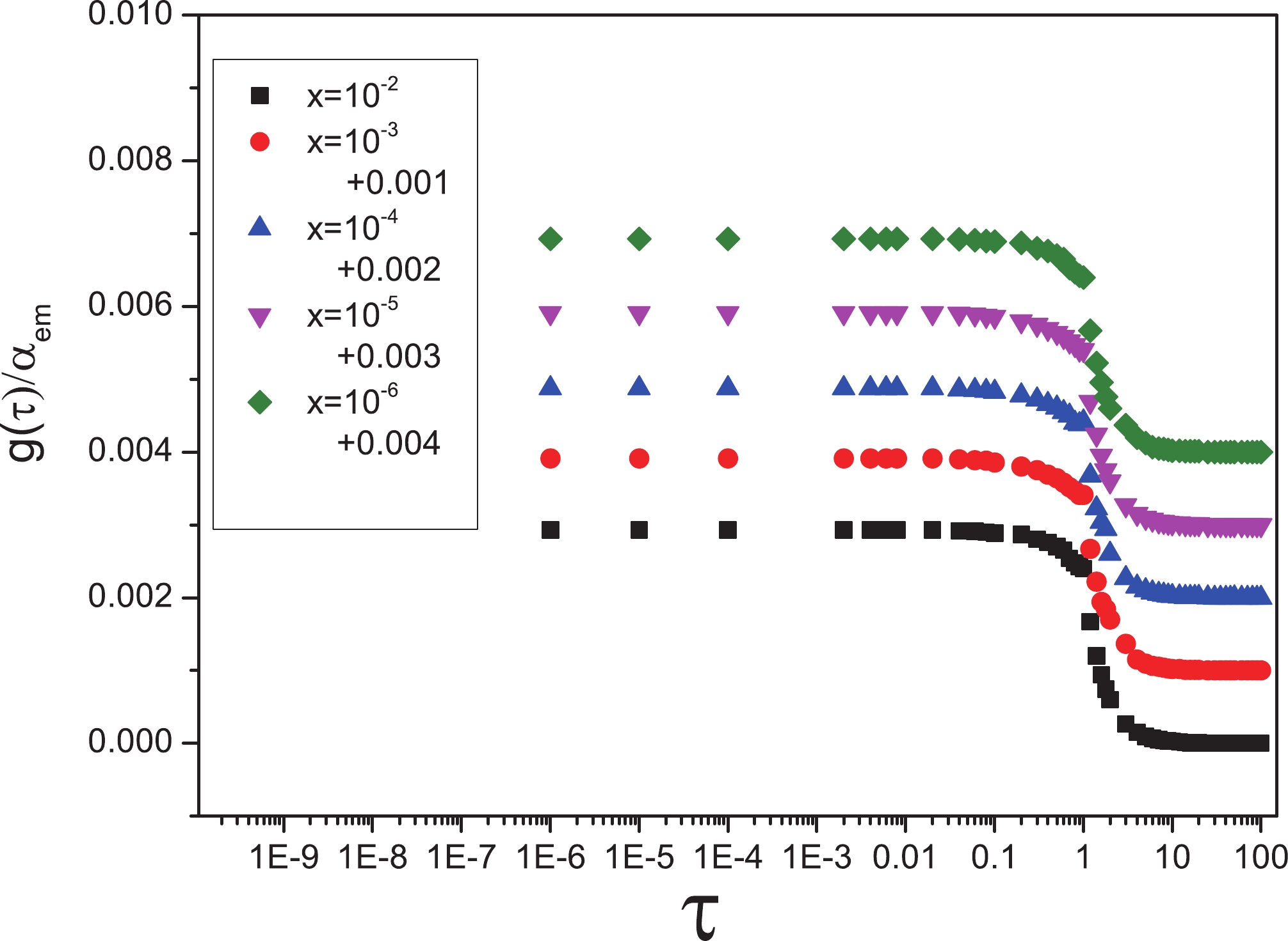Figure1. (color online) Ratio $ \dfrac{g(\tau)}{\alpha_{em}} $ for symmetric pairs with different x values belonging to the range $ 10^{-6}-10^{-2} $ to the $ \tau $ variable for light flavors.

$ \dfrac{g(\tau)}{\alpha_{em}} \sim 1 \longrightarrow \dfrac{g(\tau)}{\alpha_{em}} \sim \dfrac{1}{\tau^{2}}. $

(21)

The other limit state occurs when one of the components of the pair carries a large part of the transverse momentum. The color dipole created in this case is called the asymmetric pair. We note the condition $ \varepsilon r<1 $ in Eq. (7) is fulfilled only if $ z<\dfrac{1}{r^{2}Q^{2}} $, and there must also be a cut-off such as $ \mu^{2} \simeq 4m_{q}^{2} $ on the energy. Where the asymmetric dipole size is smaller than the saturation radius, we have

$ \begin{aligned}[b] \dfrac{{\rm d}\sigma^{D}_{\rm tot}}{{\rm d}t}\vert_{t = 0} =& \dfrac{{\rm d}\sigma^{D}_{T}}{{\rm d}t}\vert_{t = 0}+\dfrac{{\rm d}\sigma^{D}_{L}}{{\rm d}t}\vert_{t = 0}, \\ =& \dfrac{3\alpha_{em}}{32\pi^{3}}\sigma^{2}_{0}\sum\limits_{q} e_{q}^{2}\Bigg \{ \int_{1/\mu^{2}}^{1/Q^{2}}{\rm d}^{2}r\varepsilon^{2}\left(\dfrac{1}{\varepsilon^{2}r^{2}}\right) \\ & \times \int_{0}^{\textstyle\frac{1}{r^{2}Q^{2}}}{\rm d}z(z^{2}+(1-z)^{2})\left(\dfrac{r^{2}}{R_{0}^{2}(x)}\right)^{2} \\ & + \int_{1/\mu^{2}}^{1/Q^{2}}{\rm d}^{2}r\int_{0}^{\textstyle\frac{1}{r^{2}Q^{2}}}{\rm d}z 4Q^{2}z^{2}(1-z)^{2}\left(\dfrac{r^{2}}{R_{0}^{2}(x)}\right)^{2} \Bigg \}, \\ & +\int_{1/\mu^{2}}^{1/Q^{2}}{\rm d}^{2}r m_{q}^{2}\int_{0}^{\textstyle\frac{1}{r^{2}Q^{2}}}{\rm d}z\left(\dfrac{r^{2}}{R_{0}^{2}(x)}\right)^{2} \\ =& \dfrac{3\alpha_{em}}{32\pi^{2}}\sigma^{2}_{0}\dfrac{\sum\limits_{q} e_{q}^{2}}{Q^{4}R_{0}^{4}(x)}\Bigg \{ \dfrac{29}{15}+\dfrac{1}{3}\log\left(\dfrac{\mu^{2}}{Q^{2}}\right) \\ &- \dfrac{4\mu^{2}}{3Q^{2}}+\dfrac{2\mu^{4}}{5Q^{4}}+\dfrac{m_{q}^{2}}{2Q^{2}}\left(1-\dfrac{Q^{4}}{\mu^{4}}\right) \Bigg \}. \end{aligned} $

(22)

According to the high power of the virtuality, this function falls much faster than the corresponding case in small pairs and the interaction is almost unexpected. The universal function in this case is given by

$\begin{aligned}[b] g(\tau) =& \dfrac{3\alpha_{em}}{32\pi^{2}}\dfrac{1}{\tau^{2}}\sum\limits_{q} e_{q}^{2}\Bigg \{ \dfrac{29}{15}+\dfrac{1}{3}\log\left(\dfrac{\mu^{2}}{Q^{2}}\right) \\ &- \dfrac{4\mu^{2}}{3Q^{2}}+\dfrac{2\mu^{4}}{5Q^{4}}+\dfrac{m_{q}^{2}}{2Q^{2}}\left(1-\dfrac{Q^{4}}{\mu^{4}}\right) \Bigg \}. \end{aligned} $

(23)

Finally, we investigate the asymmetric pair with large size in comparison to the saturation radius:

$ \begin{aligned}[b] \dfrac{{\rm d}\sigma^{D}_{\rm tot}}{{\rm d}t}\vert_{t = 0} =& \dfrac{{\rm d}\sigma^{D}_{T}}{{\rm d}t}\vert_{t = 0}+\dfrac{{\rm d}\sigma^{D}_{L}}{{\rm d}t}\vert_{t = 0}, \\ =& \dfrac{3\alpha_{em}}{32\pi^{3}}\sigma^{2}_{0}\sum\limits_{q} e_{q}^{2}\Bigg \{ \int_{1/ \mu^{2}}^{R_{0}^{2}}{\rm d}^{2}r\varepsilon^{2}\left(\dfrac{1}{\varepsilon^{2}r^{2}}\right) \\ &\times \int_{0}^{\textstyle\frac{1}{r^{2}Q^{2}}}{\rm d}z(z^{2}+(1-z)^{2})\left(\dfrac{r^{2}}{R_{0}^{2}(x)}\right)^{2} \\ &+\int_{1/ \mu^{2}}^{R_{0}^{2}}{\rm d}^{2}r m_{q}^{2}\int_{0}^{\textstyle\frac{1}{r^{2}Q^{2}}}{\rm d}z\left(\dfrac{r^{2}}{R_{0}^{2}(x)}\right)^{2} \\ & + \int_{R_{0}^{2}}^{1/Q^{2}}{\rm d}^{2}r\varepsilon^{2}\left(\dfrac{1}{\varepsilon^{2}r^{2}}\right)\int_{0}^{\textstyle\frac{1}{r^{2}Q^{2}}}{\rm d}z(z^{2}+(1-z)^{2}) \\ &+\int_{R_{0}^{2}}^{1/Q^{2}}{\rm d}^{2}r m_{q}^{2}\int_{0}^{\textstyle\frac{1}{r^{2}Q^{2}}}{\rm d}z \\ &+ \int_{1/ \mu^{2}}^{R_{0}^{2}}{\rm d}^{2}r\int_{0}^{\textstyle\frac{1}{r^{2}Q^{2}}}{\rm d}z 4Q^{2}z^{2}(1-z)^{2}\left(\dfrac{r^{2}}{R_{0}^{2}(x)}\right)^{2} \\ & + \int_{R_{0}^{2}}^{1/Q^{2}}{\rm d}^{2}r\int_{0}^{\textstyle\frac{1}{r^{2}Q^{2}}}{\rm d}z 4Q^{2}z^{2}(1-z)^{2} \Bigg \}, \\ =& \dfrac{3\alpha_{em}}{32\pi^{2}}\sigma^{2}_{0}\sum\limits_{q} e_{q}^{2}\Bigg \{ \dfrac{-83}{90}+\dfrac{2}{R_{0}^{2}Q^{2}} \\ & +\dfrac{1}{R_{0}^{4}Q^{4}}\left(\dfrac{1}{6}+\dfrac{1}{3}\log(\mu^{2}R_{0}^{2})-\dfrac{4\mu^{2}}{3Q^{2}}+\dfrac{2\mu^{4}}{5Q^{4}}\right) \\ &+\dfrac{8}{9R_{0}^{6}Q^{6}}-\dfrac{1}{5R_{0}^{8}Q^{8}}+\dfrac{m_{q}^{2}}{2Q^{2}}1+\log\left(\dfrac{1}{Q^{2}R_{0}^{2}}\right) \Bigg \}, \end{aligned} $

(24)

so the universal function by ignoring the logarithmic sentence is

$ \begin{aligned}[b] g(\tau) =& \dfrac{3\alpha_{em}}{32\pi^{2}} \sum\limits_{q} e_{q}^{2}\Bigg \{ \dfrac{-83}{90}+\dfrac{2}{\tau}+\dfrac{1}{\tau^{2}}\Bigg(\dfrac{1}{6}-\dfrac{4\mu^{2}}{3Q^{2}} \\ &+ \dfrac{2\mu^{4}}{5Q^{4}}\Bigg)+\dfrac{8}{9\tau^{3}}-\dfrac{1}{5\tau^{4}}+\dfrac{m_{q}^{2}}{2Q^{2}} \Bigg \}. \end{aligned} $

(25)

The ratio $ \dfrac{g(\tau)}{\alpha_{em}} $ for the universal functions (23) and (25) in terms of the scaling variable has been plotted in Fig. 2 with different x values for light quarks. According to these diagrams, we can conclude that the diffractive contribution of asymmetric pairs dominates in the saturation limit, so for $ 0< \tau <1 $, the system is connected to a heavily absorbed diffractive event.
Figure2. (color online) Ratio $ \dfrac{g(\tau)}{\alpha_{em}} $ for asymmetric pairs with different x values belonging to the range $ 10^{-6}-10^{-2} $ with respect to the $ \tau $ variable for light flavors.

At high energy, heavy flavors are useful, in agreement with the experimental data. A common method of study of heavy production is based on the ratio method, which is associated with geometrical scaling [22]. In the previous section, we obtained the diffractive cross section quantitatively and showed by plotting Figs. 1 and 2 that geometrical scaling is established for light quarks. Now, we assume the summation over flavors expands to include the charm quark with $ m_{c} = $ 1.5 GeV and plot the corresponding fraction $ \dfrac{g(\tau)}{\alpha_{em}} $ in Fig. 3. According to these diagrams, we see there is no dependence on x, and all curves almost fall onto one; in other words, the geometrical scaling is confirmed. The main cause of the increase in value of this function is that the charm quark, because of its high mass, is saturated at a higher order.
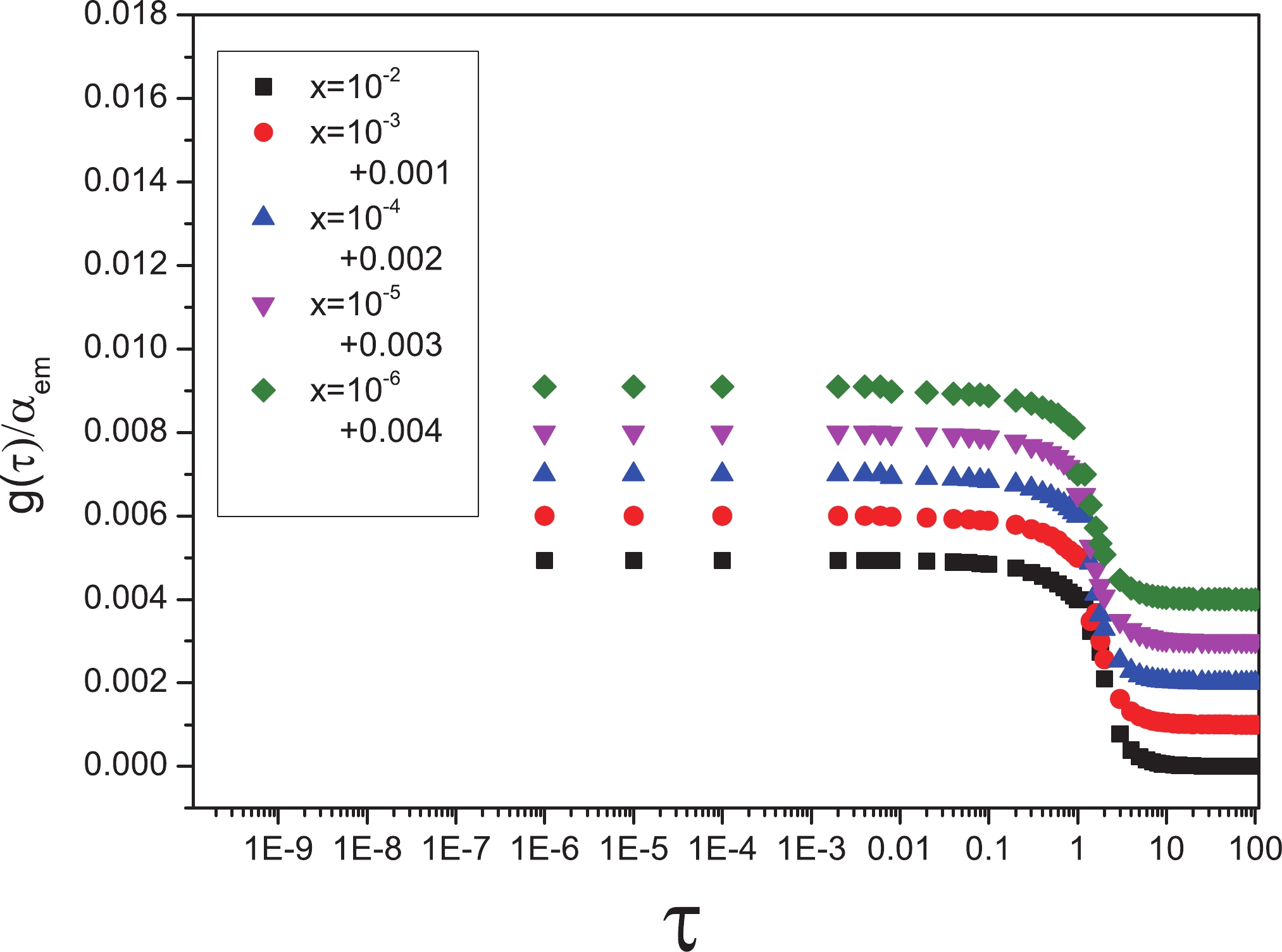Figure3. (color online) Ratio of $ \dfrac{g(\tau)}{\alpha_{em}} $ considering light and charm flavors of symmetric dipoles with different x values belonging to the range $ 10^{-6}-10^{-2} $ with respect to the $ \tau $ variable.

Figure 4, considering the bottom quark with $ m_{b} = 4.75\; {\rm{GeV}} $ and active flavors, shows that these diagrams behave similarly to those in Figs. 1 and 3; therefore, the geometrical scaling is fulfilled.
Figure4. (color online) Ratio of $ \dfrac{g(\tau)}{\alpha_{em}} $ considering light, charm, and bottom flavors of symmetric dipoles with different x values belonging to the range $ 10^{-6}-10^{-2} $ to the $ \tau $ variable.

We note that, as heavy production appears in the feature of a symmetric dipole, universal functions (16) and (18) are used in plotting the diagrams.
According to the H1 and ZEUS reports, the charm component of the structure function includes a significant fraction of the proton structure function [23, 24]. We calculate the contribution of this flavor in the diffractive cross section

$ \dfrac{\dfrac{{\rm d}\sigma_{c}^{D}}{{\rm d}t}\vert_{t = 0} }{\dfrac{{\rm d}\sigma ^{D}}{{\rm d}t}\vert_{t = 0}} = \dfrac{ g_{c}(\tau) }{g(\tau)} = \dfrac{\delta_{qc}\bigg ( g(\tau) \bigg )}{g(\tau)}, $

(26)

where the $ \delta_{qc} $ function chooses the charm quark from all active flavors. The $ c\overline{c} $ pair dominates in small size dipoles with $ r<R_{0} $; therefore,

$ \begin{aligned}[b]&\dfrac{\dfrac{{\rm d}\sigma_{c}^{D}}{{\rm d}t}\vert_{t = 0} }{\dfrac{{\rm d}\sigma ^{D}}{{\rm d}t}\vert_{t = 0}} = \dfrac{ g_{c}(\tau) }{g(\tau)} = \\ & \dfrac{e_{c}^{2}\left(\dfrac{17}{45}+\dfrac{m_{c}^{2}}{3Q^{2}}\right)}{e_{c}^{2}\left(\dfrac{17}{45}+\dfrac{m_{c}^{2}}{3Q^{2}}\right)+(e_{u}^{2}+e_{d}^{2}+e_{s}^{2})\left(\dfrac{17}{45}+\dfrac{(0.140)^{2}}{3Q^{2}}\right)}. \end{aligned} $

(27)

The average value of charm production in the diffractive process, assuming $ 0.037\leqslant r_{c}\leqslant 0.13\; {\rm{fm}} $, is approximately 40 percent according to Fig. 5. This figure shows that the corresponding fraction is independent of x and $ Q^{2} $, and all curves fall onto one.
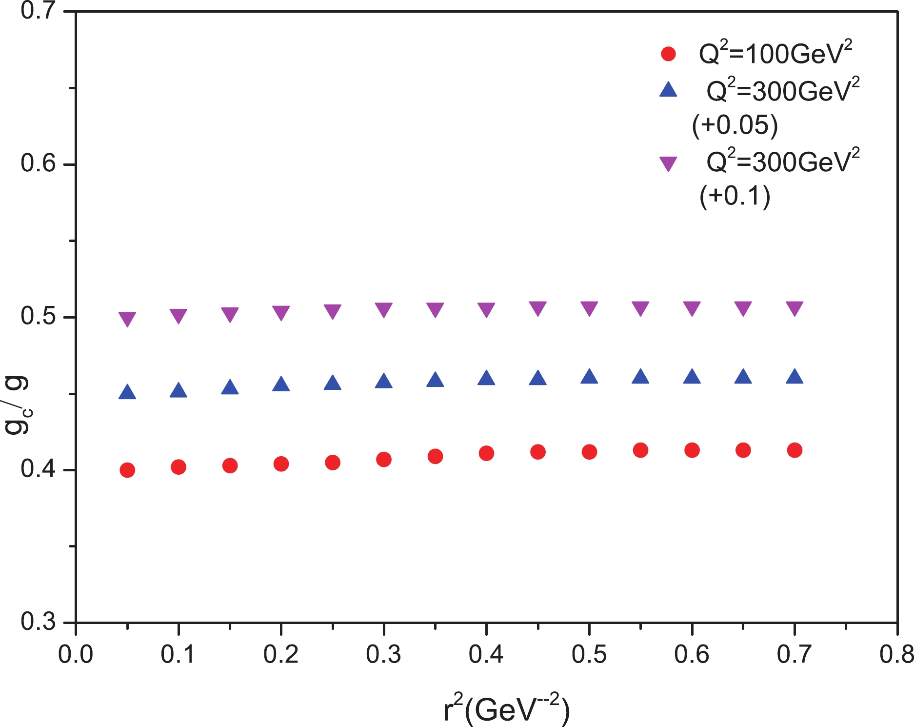Figure5. (color online) Contribution of the charm quark in the diffractive cross section for $ Q^{2} = 100, \; 200 \; {\rm{and}} \; 300\; {\rm{GeV}}^{2} $.

We can calculate this fraction to estimate the bottom production $ b\bar{b} $ as

$ \dfrac{\dfrac{{\rm d}\sigma_{b}^{D}}{{\rm d}t}\vert_{t = 0} }{\dfrac{{\rm d}\sigma ^{D}}{{\rm d}t}\vert_{t = 0}} = \dfrac{ g_{b}(\tau) }{g(\tau)} = \dfrac{\delta_{qb}\bigg ( g(\tau) \bigg )}{g(\tau)}, $

(28)

$ \delta_{qb} $ selects the bottom quark from five active flavors. Therefore, the possibility of finding the bottom production becomes

$ \begin{aligned}[b]&\dfrac{\dfrac{{\rm d}\sigma_{b}^{D}}{{\rm d}t}\vert_{t = 0} }{\dfrac{{\rm d}\sigma ^{D}}{{\rm d}t}\vert_{t = 0}} = \dfrac{ g_{b}(\tau) }{g(\tau)} = \\ & \dfrac{e_{b}^{2}\left(\dfrac{17}{45}+\dfrac{m_{b}^{2}}{3Q^{2}}\right)}{e_{b}^{2}\left(\dfrac{17}{45}+\dfrac{m_{b}^{2}}{3Q^{2}}\right)+e_{c}^{2}\left(\dfrac{17}{45}+\dfrac{m_{c}^{2}}{3Q^{2}}\right)+\dfrac{2}{3}\left(\dfrac{17}{45}+\dfrac{(0.140)^{2}}{3Q^{2}}\right)}, \end{aligned} $

(29)

which is approximately $ 10 $ percent in the range $ 0.014\leqslant r_{b}\leqslant 0.043\; {\rm{fm}} $ as seen from Fig. 6. In recent relations, the important element is $ \left(\dfrac{m_{q}^{2}}{Q^{2}}\right) $, which along with $ e_{q}^{2} $ includes inherent characteristics of the dipole. In addition, all curves in Fig. 6 fall ontoone, indicating that there is no dependence on x or $ Q^{2} $.
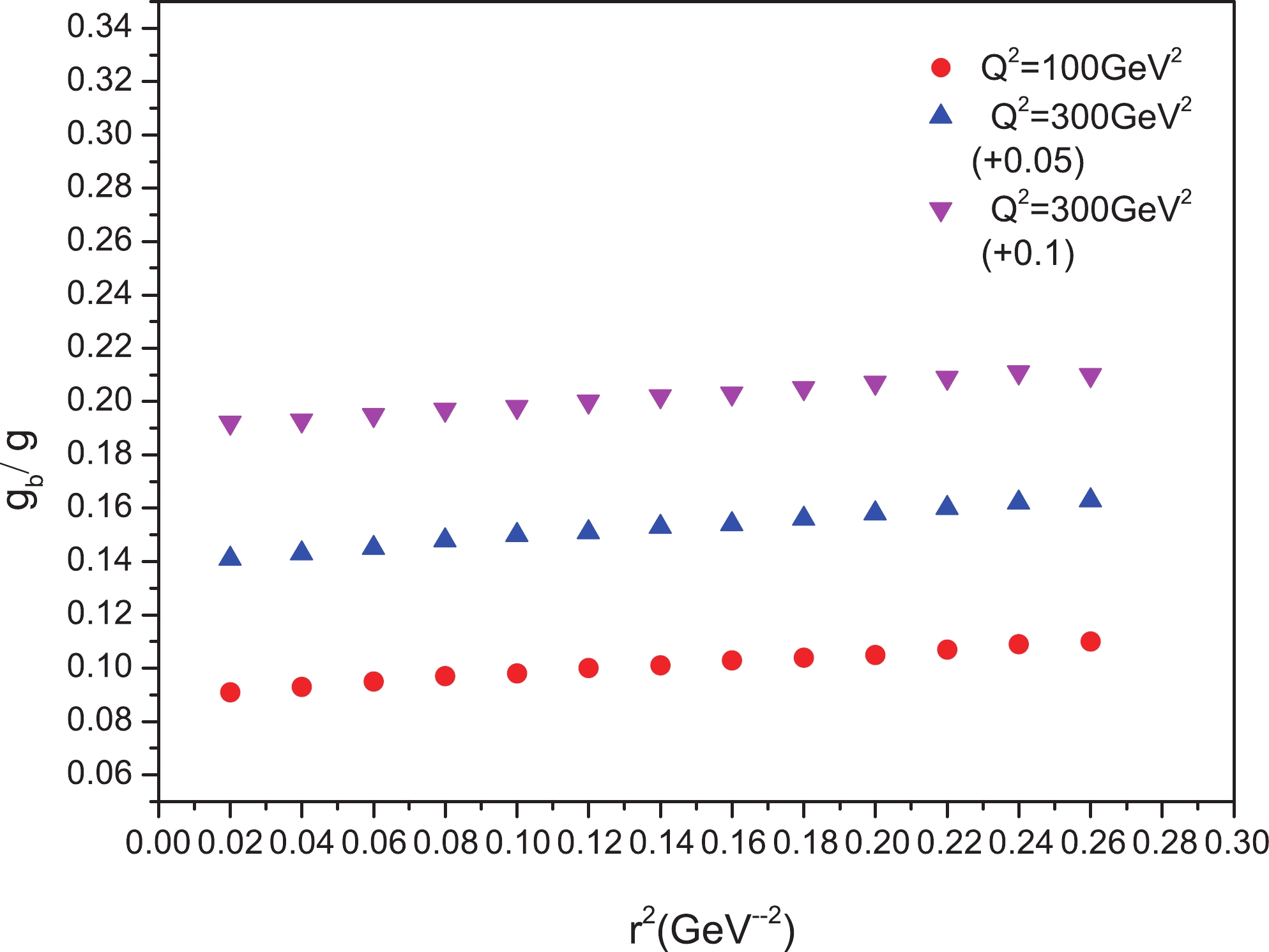Figure6. (color online) Contribution of the bottom quark in the diffractive cross section for $ Q^{2} = 100, \; 200 \; {\rm{and}} \; {300}\; {\rm{GeV}}^{2} $.

To continue, we can take a step forward and obtain the ratio of the diffractive cross section to the total cross section [21]. For symmetric dipoles with $ r < R_{0} $, we obtain

$ \begin{aligned}[b]R(\tau) =& \dfrac{\dfrac{{\rm d}\sigma^{D}_{\rm tot}}{{\rm d}t}\vert_{t = 0}}{\sigma^{\gamma^{\star}P}_{\rm tot} (x,Q^{2})} = \dfrac{\sigma_{0}^{2}g(\tau)}{\sigma_{0}f(\tau)} \\ =& \dfrac{\sigma_{0}}{16\pi \tau} \left ( \dfrac{\sum_{q} e_{q}^{2}\left(\dfrac{17}{45}+\dfrac{m_{q}^{2}}{3Q^{2}}\right)}{\sum_{q} e_{q}^{2}\left(\dfrac{11}{15}+\dfrac{m_{q}^{2}}{2Q^{2}}\right)} \right ),\end{aligned} $

(30)

and where $ r > R_{0} $, we have

$ \begin{aligned}[b]R(\tau) =& \dfrac{\dfrac{{\rm d}\sigma^{D}_{\rm tot}}{{\rm d}t}\vert_{t = 0}}{\sigma^{\gamma^{\star}P}_{\rm tot} (x,Q^{2})} = \dfrac{\sigma_{0}^{2}g(\tau)}{\sigma_{0}f(\tau)} \\ =& \dfrac{\sigma_{0}}{16\pi } \left ( \dfrac{\sum_{q} e_{q}^{2}\left(\dfrac{7}{15}-\dfrac{4\tau}{45}+\dfrac{m_{q}^{2}}{Q^{2}}\left(1-\dfrac{2\tau}{3}\right)\right)}{\sum_{q} e_{q}^{2}\left(\dfrac{4}{5}-\dfrac{4\tau}{60}+\dfrac{m_{q}^{2}}{Q^{2}}\left(1-\dfrac{\tau}{2}\right)\right)} \right ). \end{aligned} $

(31)

These ratios only relate to the size, mass, and charge of color dipoles. We have plotted them in Fig. 7 in terms of the scaling variable $ \tau $ for light flavors. In $ 0 < \tau < 1 $, we see a flat function that, for $ \tau > 1 $, reduces proportionally to $ \dfrac{1}{\tau} $, expressing that, in the diffractive event, the saturation dominates, and the interaction in the scaling region occurs rarely. It is necessary to mention that there is no dependence on x and $ Q^{2} $ [25-27]. We expect this behavior to remains when adding the contribution of heavy quarks.
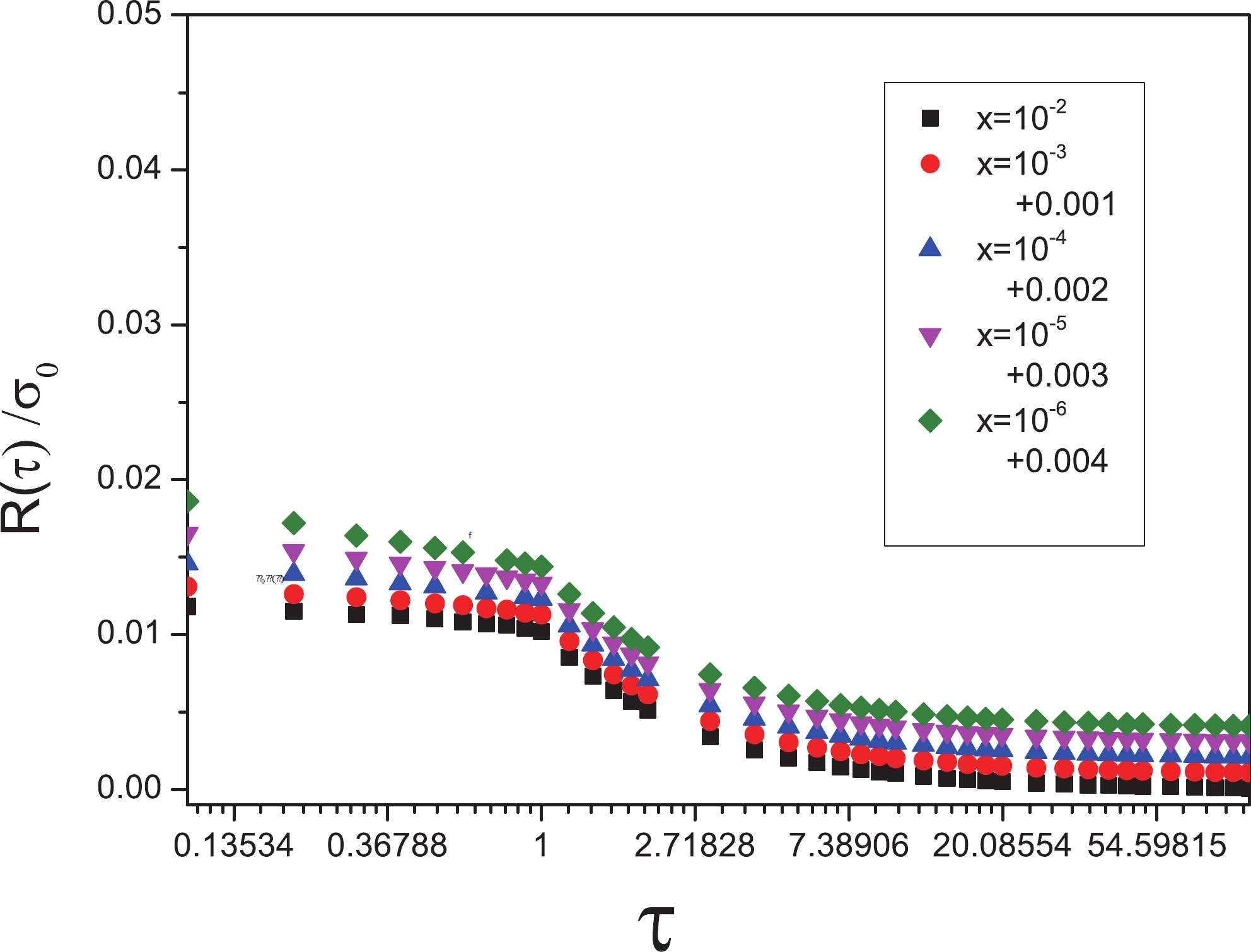Figure7. (color online) Ratio $\dfrac{1}{\sigma_{0}} \dfrac{\dfrac{{\rm d}\sigma^{D}_{\rm tot}}{{\rm d}t}\vert_{t = 0}}{\sigma^{\gamma^{\star}P}_{\rm tot}} = \dfrac{R(\tau)}{\sigma_{0}}$ with different x values belonging to the range $ 10^{-6}-10^{-2} $ with respect to the $ \tau $ variable for light flavors.

Our other suggestion for showing the ratio of the diffractive cross section to the total cross section is independent of x and $ Q^{2} $, so we plot $ \dfrac{R(\tau)}{\sigma_{0}} $ in terms of the center of mass energy of $ \gamma^{\star}p $, W, as in [12]. This quantity in Fig. 8 has been plotted for light quarks with $m_{q} = $ 140 MeV for different x values. We see a flat function for $ W>100\; {\rm{GeV}} $ that indicates the invariance of this ratio.
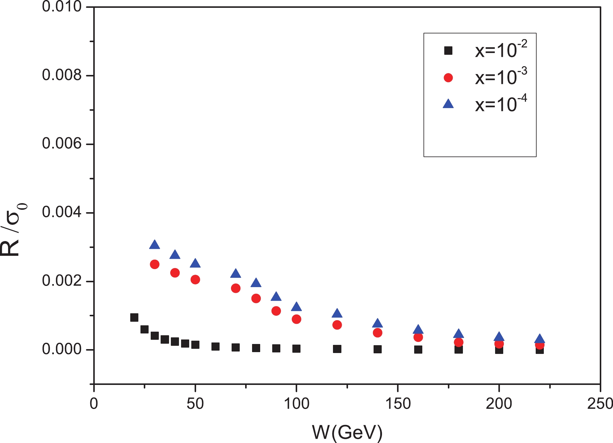Figure8. (color online) Ratio $\dfrac{1}{\sigma_{0}} \dfrac{\dfrac{{\rm d}\sigma^{D}_{\rm tot}}{{\rm d}t}\vert_{t = 0}}{\sigma^{\gamma^{\star}P}_{\rm tot}} = \dfrac{R}{\sigma_{0}}$ with different x values with respect to the center of mass energy of $ \gamma^{*}p $ for light flavors.

The color dipole picture is an effective field theory in describing the small-x limit of QCD without nonlinear sentences in the evolution equation and connects to the unitarity effect due to gluon recombination. In this analysis, we discuss diffractive deep inelastic scattering by the color dipole picture. We believe our model represents the basic dynamics because it allows us to study a wide range of data in a satisfactory way. By following the method proposed by Good and Walker, we can assume diffractive eigenstates as colorless quark-antiquark pairs that remain unchanged during scattering. The diffractive process is characterized by a final state in which an LRG is not filled with particles. The LRG in the limit of the unitarity saturation may be terminated by the absorptive correction.
We come to the conclusion that, in both the symmetric and asymmetric dipoles, the diffraction is sensitive to the saturation effect because the diffractive cross section is proportional to $ \sigma^{2}_{0} $. Fig. 1 shows there is a smooth transfer from color transparency to saturation when the scaling variable is approximately$ 1 $. Moreover, at sufficient energy, by adding the contribution of heavy flavors, this transition in Figs. 3 and 4 is observed, and the small-x saturation is proven. According to Fig. 2, we conclude that extrapolation to the diffraction process proves the saturation effect well for large-size dipoles and shows that the interaction in the scaling region occurs rarely.
The probability of the charm production in $ x<0.01 $ that directly originates from virtual photons in the diffractive process is approximately 40 percent. This impressive contribution expresses the importance of the charm cross section in colliders at high energy. The corresponding fraction for the bottom production decreases to 10 percent because of the small size and large mass of this flavor. From Figs. 5 and 6, we conclude that geometrical scaling is confirmed in the diffractive process including heavy flavors, and both of the obtained magnitudes depend on the mass, size, and charge of the involved active quarks.
The ratio of the diffractive cross section to the total cross section depicted in Fig. 7 is the other quantity that depends on the inherent characteristics of the dipoles and remains unchanged relative to the x variable. Fig. 8 offers further validation of this ratio invariance.
The significant conclusion of this work is that the diffractive event in the color dipole model probes QCD in a different way; for instance, the unitarity is an important component associated with the saturation effect that leads to a good description of the data.
In conclusion, the idea of geometrical scaling for the diffractive cross section is established. The universal functions obtained are not bounded functions and only depend on the inherent properties of dipoles.