Zhenglin Huang
, Bingjun Chen
, Lixin Qin
, Qian Zhang
, Fang Zhang
, Tieshan Wang
, Kaihong Fang ^,
,

Corresponding author: Kaihong Fang, fangkh@lzu.edu.cn

School of Nuclear Science and Technology, Lanzhou University, Lanzhou 730000, China
Received Date:2020-09-08
Available Online:2021-02-15
Abstract:The thick-target yield of the ⁹Be(d, α₀)⁷Li and ⁹Be(d, α₁)⁷Li^* reactions has been first directly measured over deuteron energies from 66 to 94 keV. The obtained S(E_i) of α₀ and α₁ have similar trends calculated by the thin-target yield, consistent with Yan’s report within the errors. Furthermore, the parametric expression of S(E) was obtained to calculate the theoretical thick target yield, and it roughly agrees with the experimental thick target yield.

HTML

--> --> -->

The measurement of basic data of a nuclear reaction plays an important role in some areas of applied physics and the test of basic theory. With the development of a low energy high-intense accelerator, light nuclear fusion research in the low energy region has attracted considerable interest. Especially, deuteron-induced reactions on light nuclei are crucial for research on a fusion reactor. The d-D and d-T reactions are the power produced by the current fusion reactor, and beryllium is considered one of the candidate materials for the first wall material in fusion reactors. For example, the first wall material of JET is layered in beryllium, and the cross sections of fast ion and plasma impurity (such as Be and B) and/or fuel ions need to be measured accurately for the diagnostic methods of nuclear reaction rate and product density in high temperature fusion plasma [1-3]. Besides, the accurate measurement of these reactions in the low energy region may be used to test the nuclear reaction theory that may provide insights into the influence of the Oppenheimer effect [4] and electron screening effect [5] on the cross section at low energies. The analysis of d-T reactions at low energies by R-matrix theory has been proved to be quite successful [6]. This method has been used in deuterium induced reactions on heavier nuclei [7].
In the astrophysical environment and fusion reactor, the reaction under several keV conditions far lower than the Coulomb barrier, occurs only depending on the tunneling effect. Thus, the cross section decreases sharply with the decreasing energy, and it is a challenge to directly measure the cross section, which can only be deduced by extrapolation. In general, the cross section is expressed by the S-factor (σ(E)=S(E)E^?1exp(?2πη(E))), which does not change rapidly with respect to energy [8].
In recent decades, only a few studies have been conducted on d-⁹Be reactions. In 1972, Jiang et al. [9] measured the total cross section for the ⁹Be(d, α₀/α₁) reactions between energies (laboratory system) of 0.15 and 2.5 MeV with an energy step of ?E=200 keV. Bertrand et al. [10] only measured the cross section of the d-⁹Be reaction in the energy (Lab system) region from 300 keV to 1 MeV; Annegarn et al. [11] found an energy level of ¹¹B at 16.43 MeV from the excitation function of the d- ⁹Be reaction. Only Yan’s work [12] reported on the cross section and angular distribution of the d-⁹Be reaction in the energy region from 69 to 132 keV; some of the results of angular distribution showed significant anisotropy. Then, they used the distorted wave Born approximation calculations to fit this anisotropy, which was modified by the additional short-range term [12]. However, the energy step that they selected was so large (?E = 15 keV) that it resulted in inevitable errors in the calculations of effective energy and S(E). Consequently, the cross section of the d-⁹Be reaction needs to be measured at an energy as low as possible, with a small energy step.
In this work, we measured the excitation function in the energy range from 66 to 94 keV and obtained the expression of S(E) of the ⁹Be(d, α₀)⁷Li and ⁹Be(d, α₁)⁷Li^* reactions. Details of the experimental setup and procedure are presented in the next chapter. Finally, the data analysis and discussion are shown in chapter III.

An accelerator with low energy and high beam current was used to carry out the experiment; it belongs to the Research Center for Electron Photon Science of Tohoku University and includes a duo-plasmatron ion source, a beam extraction system, an analysis magnet (30 degrees), focusing lenses, an electrode used to accelerate and decelerate ions, and a deflection magnet, which can adjust the beam direction. 25 kV of power was supplied for the duo-plasmatron ion source, which provided the high current beam (about 1 mA). More experimental details are available in the references [13-20]. The configuration of the reaction target chamber is shown in Fig. 1.
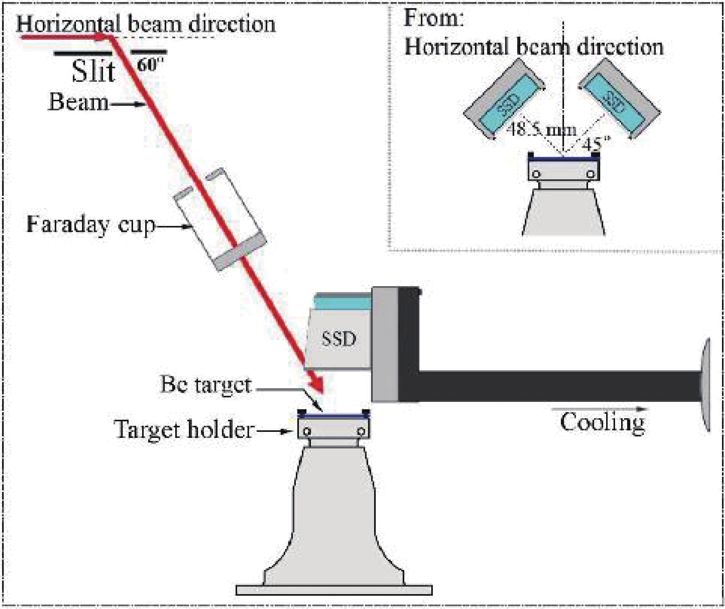Figure1. (color online) Configuration of the reaction target chamber.

We measured the thick target yield of α₀/α₁ particles from the ⁹Be(d, α₀)⁷Li and ⁹Be(d, α₁)⁷Li^* reactions in the present work from 66 to 94 keV with an energy step of ?E = 2 keV and a fluctuation range of beam energy within 30 eV. The angle between the deuteron beam and the horizontal direction was 60 degrees after the beam passed through the bending magnet; then, a beam spot with a diameter of 8 mm was formed on the target. In this experiment, two silicon surface barrier detectors were used and installed symmetrically relative to the beam direction, and the detection angle was 127 degrees. We used the ⁶Li(d, α)⁴He reaction at E_d-lab = 90 keV to calibrate the solid angle (ΔΩ/4π), which is about 3%. In addition, Al foils with thickness values of 0.8 and 2.8 μm were used to prevent the elastic scattering deuterons from entering the detector directly and separate the overlapping peaks. The 0.8 μm-thick Al foil was used for all the beam energy, while the 2.8 μm-thick Al foil was only used for beam energies from 66 to 90 keV. In the present work, we used the aluminum detector bracket and cooled it to 5 ℃ with water to maintain the best performance of the detector.
A Faraday cup (FC) was installed in the front of the target to obtain the number of projectiles and monitor the beam current directly. In order to avoid the effect of temperature, the beams with different energies should keep the same power. With the decrease in beam energy, the beam intensity should be increased appropriately. However, when the beam intensity is high to a certain extent, the dead time of the detector is too large, so the detection efficiency may be reduced, which may introduce more errors. The beam current stability was monitored intensively to reduce the effect of secondary electrons escaping the target. Before each bombardment (10 seconds) on the beryllium target, FC was inserted for 4 seconds. The last 3 seconds were used to measure the beam current, and then, the FC was pulled out, and the next bombardment occurred after waiting for 2 seconds. During the experiment, the intensity of the beam current during the measurement interval was obtained by calculating the average beam intensity of adjoining monitoring points. The fluctuation range of beam intensity was less than 5%, which did not affect the integrated incident charges due to the interval measurement.
Meanwhile, we monitored the overall deuteron energies of the beam spot position. Two detectors, symmetrically placed with respect to the beam direction mentioned above, were used to eliminate the influence of the left and right (perpendicular to beam direction) movements of the beam spot on the detection efficiency. The effects of the forward and backward (parallel to the direction of beam current) movements of the beam spot on the detection efficiency was about 3.0% ± 0.2 %. Finally, we found that the overall range of motion of the beam spot was less than 2 mm.
The beryllium target used in this experiment was 99% pure and fixed at the chamber, as shown in Fig. 1. The vacuum is about 10^?5 Pa during bombardment. In the experiment, the target contamination must be considered (e.g., the stopping power and screening effect). Therefore, before and after each bombardment, the α-yield at a specific energy point (70 keV) was chosen to monitor the target environment. The target was unused when the α-yield decreased significantly. Generally, we use a high-intensity beam to bombard the target or use fresh targets to ensure the data availability. For example, consider improving the target environment; a high-current (100 μA) 70 keV deuteron beam (D+) was used to sputter the target. Finally, we used the Secondary-Ion Mass Spectroscopy (SIMS) to analyze all the samples and found that only about 6% D-atoms are deposited on bombard targets compared with that on non-irradiated ones.

Figure 2 shows the emission energy spectrum of charged particles of the d-⁹Be reaction at 90 keV. The α-particles come from the ⁹Be(d, α₀)⁷Li and ⁹Be(d, α₁)⁷Li^* reactions, while the protons come from the reactions of ⁹Be(d, p₀)¹⁰Be and ⁹Be(d, p₁)¹⁰Be^* and the tritium from the reaction of ⁹Be(d, t)⁸Be. The emphasis of the current work is on the peaks of alpha particles (α₀ and α₁). It is clearly seen that the peaks separate from each other with a low background. The thick-target yield of α-particles from the ⁹Be(d, α₀)⁷Li and ⁹Be(d, α₁)⁷Li^* reactions is shown in Fig. 3.
Figure2. The energy spectrum of charged particles emitted from the d-⁹Be reaction with a beam energy of 90 keV.

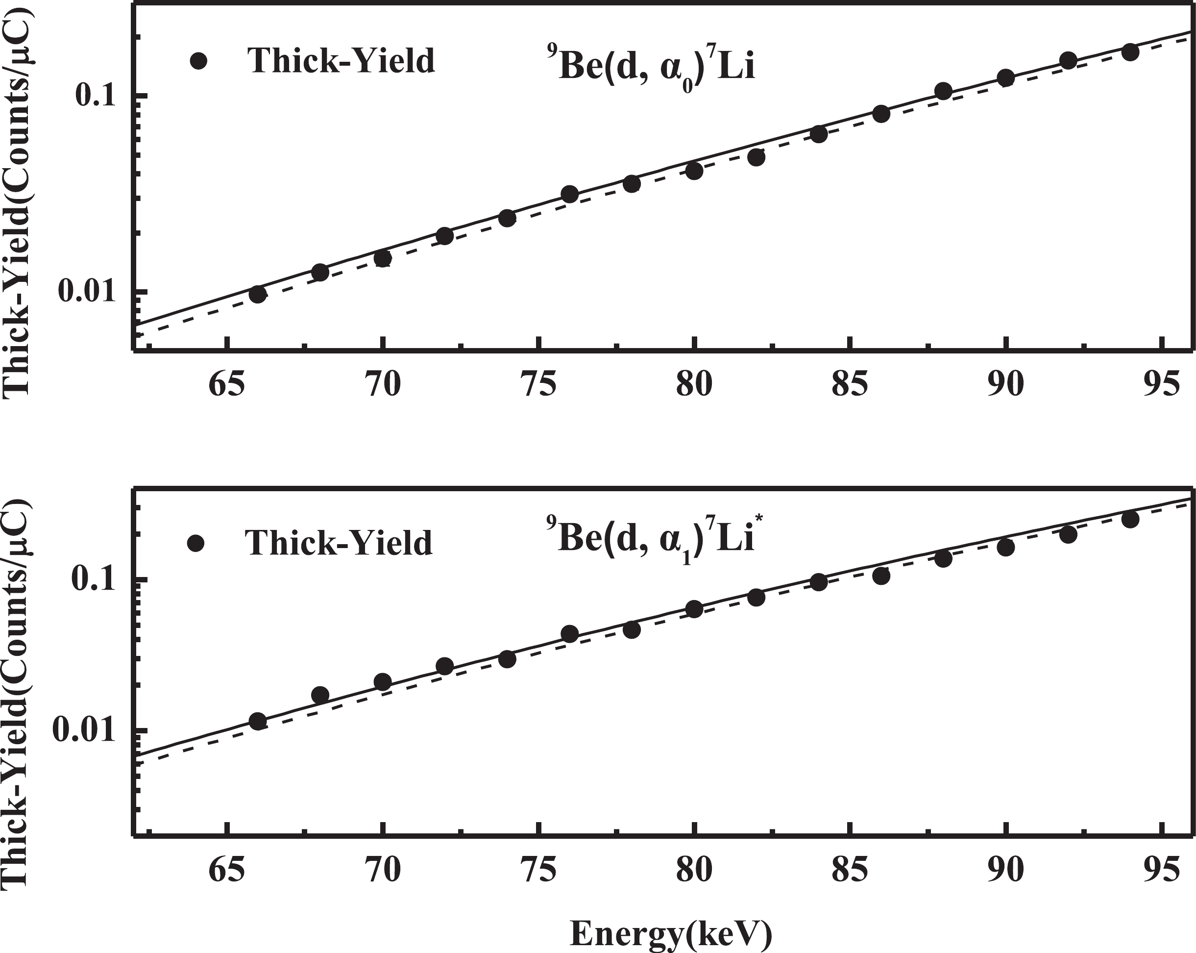Figure3. The thick-yield of an α particle from ⁹Be (d, α₀)⁷Li (top) and ⁹Be (d, α₁) ⁷Li^* (bottom) reactions. The solid curve and dashed curve denote with and without the screening effect, respectively.

According to Eq. (1), the thick-target α-particle yield [Y_α^thick (E_d)] is related to S_screen(E) and can be expressed as

$\begin{aligned}[b] Y_\alpha ^{\rm thick} =& \frac{{{N_d}{N_t}\Delta {\varOmega _{\rm lab}}}}{{4\pi }}\mathop {\mathop \int\nolimits_0^{{E_d}} } \frac{{{\rm d}{\varOmega _{\rm c.m.}}}}{{{\rm d}{\varOmega _{\rm lab}}}}W(E){S_{\rm screen}}(E) \\&\times \exp( - 2\pi {\rm{\eta }}) \times {\left(\frac{{{\rm d}E}}{{{\rm d}x}}\right)^{ - 1}}{\rm d}E , \end{aligned}$

(1)

where N_d is the number of incident deuterons, N_t is the number density of target atoms, ?Ω_lab is the solid angle, dΩ_c.m./dΩ_lab is the ratio of the solid angle at the center of mass system to the laboratory system, S_screen(E_c.m.) the astrophysical factor, which is a function of E_c.m. in the center of mass system, W(E) [12] is the angular distribution, which is the Legendre polynomial of E, and dE/dx is the energy loss of deuterium in Beryllium calculated by the SRIM code [21].
Therefore, the S_screen(E_i) can be calculated using the thin-target yield differentiated by two adjacent thick-target yields.

$ {{Y}}_{{\alpha}}^{{\rm thin}}\left({{E}}_{{0}}\right){=}{{Y}}_{{\rm exp}}{(}{{E}}_{{0}}{)}{-}{{Y}}_{{\rm exp}}{(}{{E}}_{{0}}{-\Delta E}{)}. $

(2)

According to Eq. (1) and Eq. (2), the thin target yield can be expressed as

$\begin{aligned}[b] {{Y}}_{{\alpha}}^{{\rm thin}}{(}{{E}}_{{0}}{)}{=}&\frac{{{N}}_{{d}}{{N}}_{{t}}{{\Delta \varOmega}}_{{\rm lab}}}{{4\pi}}{ \times S}{(}{{E}}_{{\rm eff}}{)}{ \times }\mathop {\mathop \int\nolimits_{{{E_0} - \Delta E}}^{{E_0}} } \frac{{\rm d}{{\varOmega}}_{{\rm c.m.}}}{{\rm d}{{\varOmega}}_{{\rm lab}}}{W}\left({E}\right)\frac{{1}}{{{E}}_{{\rm c.m.}}}\\&{ \times \exp}{(}{-2\pi \eta }{(}{{E}}_{{\rm c.m.}}{))}{ \times }{\left(\frac{{{\rm d}E}}{{{\rm d}x}}\right)}^{{-1}}{{\rm d}E}, \end{aligned}$

(3)

where E_eff is the effective deuteron energy in this energy step, which can be calculated by [10]:

$ {E_{\rm eff}} = {E_0} - \Delta E + \Delta E\left\{ { - \frac{{{\sigma _2}}}{{{\sigma _1} - {\sigma _2}}} + {{\left\{ {\frac{{{\sigma _1}^2 + {\sigma _2}^2}}{{2{{({\sigma _1} - {\sigma _2})}^2}}}} \right\}}^{\frac{1}{2}}}} \right\}, $

(4)

where σ₁ is the cross section at E₀, and σ₂ is the cross section for E₀-?E.
Then, the S(E_i) can be obtained from Eq. (4), which is shown in Table 1. It is found that S(E_i) only slightly fluctuate from our expectation. Since the data of most works in high energy region are far from this work, we only compare with the results of Yan’s work, as shown in Fig. 4. To calculate the thick target yield, the S(E_i) were fitted using the parametric S_bare(E) = a + b·E + c·E² + d·E³ multiplied by the enhancement factor f (E, U_s):

Ec.m./keV	9Be(d, α0)7LiS(Ei)/(MeV·b)	9Be(d, α1)7Li*S(Ei)/(MeV·b)
55.6	9.0±2.3	29.3±4.5
57.3	8.9±1.4	22.2±2.8
58.9	9.0±1.8	15.3±3.4
60.5	9.5±1.1	23.1±2.3
62.2	7.1±1.5	17.9±3.2
63.8	4.7±1.1	16.7±2.2
65.5	4.9±1.1	19.6±2.4
67.1	6.7±1.0	17.1±2.0
68.7	7.9±1.0	12.7±2.0
70.4	8.3±1.0	14.6±2.5
72.0	6.9±1.0	16.4±1.7
73.6	6.2±0.9	14.2±2.0
75.3	4.8±0.9	17.2±1.4
Note: The error values include the statistical error of the alpha particle number, detection efficiency, and beam current measurement. Besides, for all S(Ei), the angular distribution introduces a 4% uncertainty; an error of 3% comes from the change in target environment in the experiment; a 1% uncertainty is due to the uncertain detection angle, and another error of 7.4% occurs in the stopping power (5.4%, mean errors).

Table1.The S factor and its error of the ⁹Be (d, α₀)⁷Li and ⁹Be (d, α₁) ⁷Li^* reactions.

Figure4. (color online) Comparison of S(E_i) factor between this work (solid black circles) and previous work (solid red circles). The top one is the S factor of ⁹Be(d, α₀)⁷Li reaction, and the bottom one is the S factor of ⁹Be(d, α₁)⁷Li^* reaction. The solid and dashed curves are the S_screen(E) and the S_bare(E), respectively.

$ {f}{(}{{E}{,}{U}}_{{s}}{)}{=}\frac{{{\sigma}}_{{\rm screen}}{(}{E}{)}}{{{\sigma}}_{{\rm bare}}{(}{E}{)}}{=}\frac{{{S}}_{{\rm screen}}{(}{E}{)}}{{{S}}_{{\rm bare}}{(}{E}{)}}{ \approx }\frac{{E}}{{E+}{{U}}_{{s}}}{\rm exp}\left({\pi \eta }\frac{{{U}}_{{s}}}{{E}}\right), $

(5)

where U_s = 512 eV is the electron screening potential from our previous work [14], S_bare(E) is the bare nucleus S factor without U_s. Usually, U_s is considered the energy of the incident particle (i.e., S_screen(E) = S_bare(E) ? f (E, U_s) = S_bare(E + U_s)). a, b, c, and d are the coefficients of the polynomial term. Clearly, the enhancement factor f(E, U_s) increases sharply with the decreasing energy, especially at a low energy region, owing to the exponential term.
The results of S_screen(E) and S_bare(E) are the solid and dashed curves shown in Fig. 4, respectively. It is clear that the polynomials can describe the trend of the S factor well in the energy region presented in this work (below 140 keV), while it is difficult to predict the S(E) of the ⁹Be(d, α) reaction at the Gamow window by extrapolation because it may lead to considerable uncertainty due to the significant statistical error in a lower energy region (below 50 keV). Finally, we used the polynomial to calculate the thick target yields. However, it cannot explain the experimental thick target yield well; as shown in Fig. 3, the solid curve and dashed curve denote with and without screening effect, respectively. The main reason is the errors of S(E_i). Therefore, more measurements in the low energy region are needed, especially for E < 50 keV.

The thick target yields of the ⁹Be(d, α₀)⁷Li and ⁹Be(d, α₁)⁷Li^* reactions are measured from E=66 to 94 keV, and we first report on the S-factors calculated by the thin target yield. The S-factor of this experiment is consistent with Yan’s result within the errors. S(E_i) are fitted via the polynomial S(E), which can describe the S(E_i) well. The thick target yields (with U_s and without U_s) are calculated by the fitting expression. Due to the absence of data from 100 to 300 keV and below 50 keV, it is difficult to explain the physical mechanism and obtain the S(E) in the Gamow energy region. Therefore, more experiments of the d-⁹Be reaction should be performed.

The authors thank the Research Center for Electron Photon Science in Tohoku University, Japan, for their hospitality during the experiments.