Y. J. Li ^1,
, X. Fang ^2,,
, B. Bucher ^3,
, K. A. Li ^4,5,
, L. H. Ru ^4,5,
, X. D. Tang ^4,5,
,

Corresponding author: X. Fang, fangx26@mail.sysu.edu.cn

1.China Institute of Atomic Energy, Beijing 102413, China
2.Sino-French Institute of Nuclear Engineering and Technology, Sun Yat-sen University, Zhuhai 519082, China
3.Idaho National Laboratory, Idaho Falls, ID 83415, USA
4.Institute of Modern Physics, Chinese Academy of Sciences, Lanzhou 730000, China
5.School of Nuclear Science and Technology, University of Chinese Academy of Sciences, Beijing 100049, China
Received Date:2020-05-09
Available Online:2020-11-01
Abstract:The ¹²C+¹²C fusion reaction plays a crucial role in stellar evolution and explosions. Its main open reaction channels include $\alpha$, p, n, and ⁸Be. Despite more than a half century of efforts, large differences remain among the experimental data of this reaction measured using various techniques. In this work, we analyze the existing data using a statistical model. Our calculation shows the following: 1) the relative systematic uncertainties of the predicted branching ratios decrease as the predicted ratios increase; 2) the total modified astrophysical S-factors (S^* factors) of the p and $\alpha$ channels can be obtained by summing the S^* factors of their corresponding ground-state transitions and the characteristic $\gamma$ rays, while taking into account the contributions of the missing channels to the latter. After applying corrections based on branching ratios predicted by the statistical model, an agreement is achieved among the different data sets at E_cm > 4 MeV, while some discrepancies remain at lower energies, suggesting the need for better measurements in the near future. We find that the S^* factor recently obtained from an indirect measurement is inconsistent with the direct measurement value at energies below 2.6 MeV. We recommend upper and lower limits for the ¹²C+¹²C S^* factor based on the existing models. A new ¹²C+¹²C reaction rate is also recommended.

HTML

--> --> -->

The ¹²C+¹²C reaction at astrophysical energies is a crucial reaction for stellar evolution and explosion. For example, stars above eight solar masses can ignite the ¹²C+¹²C fusion reaction and proceed with carbon burning inside their cores when the core temperature is above 0.6 GK. These stars end their lives as Ne/O white dwarfs. More massive stars will continue the ¹²C+¹²C reaction in their shells at temperatures around 1.0-1.2 GK and eventually become supernovae. When a star explodes, a shock wave propagates through the outer layers of the dying star and initiates the explosive carbon burning, which imprints its unique nucleosynthetic patterns in the ashes of the dying star. The ¹²C+¹²C fusion reaction is considered to be the ignition reaction of type Ia supernovae [1] and superbursts. In type Ia supernovae, ignition occurs in the white dwarf core, typically at T~ 0.15-0.7 GK and $ \rho\sim $ (2-5)×10⁹ g/cm³. In type-I X-ray bursts, ash from the rp-process builds up on the surface of the neutron star with a significant amount of ¹²C (3%~10%). Heat sources in the crust of neutron star raise the temperature of the ash and eventually trigger carbon ignition at a temperature of ~0.5 GK [2] and density above 3×10⁹ g/cm³. The ignition conditions mentioned above strongly depend on the actual ¹²C+¹²C reaction rate as well as the estimation of the screening effect in dense matter [2-4].
The crucial energy range extends from a few tens of keV to $ E_{\rm cm} $ = 3 MeV [4], well below the Coulomb barrier at $ E_{\rm cm} $ = 5.5 MeV [5]. Two ¹²C nuclei fuse into the compound nuclear states of ²⁴Mg with excitation energies of 14 to 17 MeV. The compound states then decay through five channels:

$\begin{aligned}[b]^{12}{\rm{C}}{{\rm{ + }}^{{\rm{12}}}}{\rm{C}}&{ \to ^{{\rm{20}}}}{\rm{Ne + }}\alpha {\rm{ + 4}}.{\rm{62 \;MeV}}{ \to ^{{\rm{23}}}}{\rm{Na + {\rm{p}} + 2}}.{\rm{24 \;MeV}}\\&{ \to ^{{\rm{23}}}}{\rm{Mg + {\rm{n}} - 2}}.{\rm{60 \;MeV}}{ \to ^{{\rm{16}}}}{\rm{O}}{{\rm{ + }}^{\rm{8}}}{\rm{Be - 0}}.{\rm{20\; MeV}}\\&{ \to ^{{\rm{24}}}}{\rm{Mg + 14}}.{\rm{934 \;MeV.}}\end{aligned}$

The corresponding energy levels of the compound nucleus and residual nuclei are shown in Fig. 1. The energies of protons and alpha particles in the decay channels are above their Coulomb barriers when the excitation energy of the compound nucleus is above the ¹²C+¹²C separation energy. Consequently, the particle decay widths are much larger than the $ \gamma $-decay width. Therefore, the contribution of the radiative capture channel is negligible.
Figure1. Energy-level diagram for the ¹²C+¹²C system with primary exit channels at low energies. p$_{i}$, $\alpha_{i}$, and n$_{i}$ represent the protons produced with ²³Na, $\alpha$ particles produced with ²⁰Ne, and neutrons produced with ²³Mg, respectively, at the ground state (i = 0) or the $i^{\rm th}$ excited state (i = 1,2,3,...). The energies for most common characteristic $\gamma$ rays are 440 keV for ²³Na, 1634 keV for ²⁰Ne, and 450 keV for ²³Mg. Apart from these three most important channels, the ¹²C(¹²C,⁸Be)¹⁶O channel is also possible and may warrant further investigation.

¹²C(¹²C,$ \alpha $)²⁰Ne and ¹²C(¹²C,p)²³Na are the two major reaction channels at sub-barrier energies [6-8]. The measurements of ¹²C(¹²C,$ \alpha $)²⁰Ne and ¹²C(¹²C,p)²³Na atsub-barrier energies are classified into two categories: the detection of either characteristic $ \gamma $-rays or light charged particles. A summary of previously conducted experimental studies, directly measuring $ \alpha $- and p-channels of the ¹²C+¹²C reaction near stellar energies, is presented in Table 1. A pioneering particle spectroscopy experiment was performed by Patterson et al. [6], who measured the cross sections of p and $ \alpha $ using a telescope system consisting of a proportional counter and a silicon detector. Later, Mazarakis and Stephens [9] and Becker et al. [10] independently repeated the particle spectroscopy experiments using silicon detectors. Limited by the target purity and beam-induced backgrounds, these measurements were within the range of $ E_{\rm cm}> $2.7 MeV. Using a thick highly ordered pyrolytic graphite (HOPG) [11, 12] target, Zickefoose et al. [13] successfully suppressed these backgrounds and extended the particle-spectroscopy measurement of ¹²C(¹²C,p$ _{0,1} $)²³Na down to $ E_{\rm cm} $ = 2.0 MeV. No other channels were measured due to a thick degrader used in front of the detectors to control the beam-induced background.

Measurement	$E_{\rm cm}$/MeV	Beam/pμA	Target	Technique	Detection of partial $\sigma$	method to calculate total $\sigma$
Patterson [6]	3.23 – 8.75	0.017–0.17	Carbon foil with thickness of about 40 μg/cm2.	Particle spectroscopy. Protons and $\alpha$ particles were detected at four angles between 20° to 80° by a $\Delta$E-E telescope consisting of an argon proportional counter 6 cm long and a silicon surface-barrier detector 1.5 mm thick. The n-channel was measured by counting the offline $\beta$-decay of residual 23Mg above 4.25 MeV.	Total cross sections: $\sigma_{\alpha}$, $\sigma_{p}$, $\sigma_n$.	$\sigma_{\alpha}$ = sum of $\alpha_0$, $\alpha_1$, $\alpha_2$, $\alpha_3$, $\alpha_4$, $\alpha_5$; $\sigma_{p}$ = sum of $p_{0-1}$, $p_{2-6}$, $p_{7-9}$, $p_{10}$.
Mazarakis and Stephens [9]	2.55 – 5.01	$\leq$0.38	Self-supporting foils from high-purity graphite, 30, 53, and 65 μg/cm2.	Particle spectroscopy. Surface barrier Si detectors at eight angles between 20° and 90°.	Cross sections of $\alpha_0$, $\alpha_1$, $\alpha_2$, $\alpha_3$, $\alpha_4$+$\alpha_5$, $\alpha_6$, $\alpha_7$ and $p_0$, $p_1$, $p_2$, $p_3$, $p_4$+p5, $p_6$, $p_7$, $p_8$+$p_9$, $p_{10}$.	$\sigma_{\alpha}$ = $\sum \sigma_{\alpha_i}$, $\sigma_{p}$ = $\sum \sigma_{p_i}$.
Becker [10]	2.8 – 6.3	1–5	Self-supporting foils from graphite, 8 to 30 μg/cm2.	Particle spectroscopy. Nine surface barrier Si detectors at 10° to 90° (in 10° steps).	Cross sections of $\alpha_0$, $\alpha_1$, $\alpha_2$, $\alpha_3$, $\alpha_4$, $\alpha_5$, $\alpha_6$, $\alpha_7$, $\alpha_8$+$\alpha_9$, $\alpha_{10}$, $\alpha_{11}$, $\alpha_{12}$ and $p_0$, $p_1$, $p_2$, $p_3$, $p_4$+$p_5$, $p_6$, $p_7$, $p_8$+$p_9$, $p_{10}$, $p_{11}$, $p_{12}$, $p_{13}$, $p_{14}$+$p_{15}$+$p_{16}$.	$\sigma_{\alpha}$ = $\sum \sigma_{\alpha_i}$, $\sigma_{p}$ = $\sum \sigma_{p_i}$. Estimating the contributions of the missing channels with the extrapolation of the averaged S* factor at higher energies
Zickefoose [13]	2.0 – 4.0	$\leq$15	Thick target: high-purity graphite; HOPG.	Particle spectroscopy. Two $\Delta$E–E telescopes at 130° ($\Delta$E–Si detector: area A = 300 mm2, thickness t = 15 μm; E–Si detector: A = 300 mm2, t = 300 μm).	The $p_0$+$p_1$ reaction yield of the infinitely thick target was obtained with energy steps of $\Delta$E = 20 to 100 keV.	No total cross sections were given.
Kettner [14]	2.45 – 6.15	$\leq$15	Carbon targets (9 to 55 μg/cm2) were evaporated on 0.3 mm thick Ta backings.	$\gamma$-ray spectroscopy. One Ge(Li) detector at 0°.	$\gamma$-ray transitions from a large number of excited states in 20Ne, 23Na, and 23Mg were observed, providing corresponding partial cross sections.
Dasmahapatra [20]	4.2 – 7.0	$\leq$0.015	Carbon foil with thickness of about 30 μg/cm2.	$\gamma$-ray spectroscopy. Two NaI detectors, in almost 4$\pi$ geometry. The pulses from the two NaI detectors were summed via a amplifier.	Total-$\gamma$-ray-yield method.	To obtain total cross sections, the fraction $\sigma_{\gamma}$/$\sigma_{\rm total}$ from experimental data of Mazarakis and Stephens [9] was used.
Aguilera [15]	4.42 – 6.48		Amorphous C-foil deposited onto thick Ta backing. Thickness: 19.2$\pm$0.9 , 22.7$\pm$1.0 , 29.9$\pm$1.4 μg/cm2.	$\gamma$-ray spectroscopy. Two HPGe at 125° and 55°.	$\gamma$-ray cross sections of 1634, 440, and 450 keV, corresponding to ground-state transitions.	The $\alpha_0$ and $p_0$ cross section values of Becker et al.[10] were used to correct data. $\sigma_{\alpha}$ = $\sigma_{\alpha_0}$+$\sigma_{\gamma(1634)}$, $\sigma_{p}$ = $\sigma_{p_0}$+$\sigma_{\gamma(440)}$.
Spillane [16]	2.10 – 4.75	$\leq$40	Thick target: high-purity graphite.	$\gamma$-ray spectroscopy. One HPGe at 0°. The $\gamma$-ray efficiencies: (3.6%$\pm$0.4%) for $E_{\gamma}$ = 440 keV, (1.9%$\pm$0.2%) for $E_{\gamma}$ = 1634 keV.	The $\gamma$-ray thick-target yields of the 440 and 1634 keV lines with energy steps of 12.5 to 25 keV. To arrive at a thin-target yield, the thick-target yield curve was differentiated.	$\sigma_{\alpha}$ = $\sigma_{\gamma(1634)}$, $\sigma_{p}$ = $\sigma_{\gamma(440)}$.
Jiang [17]	2.68 – 4.93	$\leq$0.6	Isotopically enriched (99.9%) 12C targets with thickness of approximately 30-50 μg/cm2.	Particle-$\gamma$ coincidence technique. DSSD$_{1,2,3}$: 147°–170°, 123°–143°, 17°–32°; 25% of 4$\pi$. The $\gamma$-ray efficiencies: 9% for $E_{\gamma}$ = 440 and 7% for $E_{\gamma}$ = 1634 keV.	$\sigma_{p_1}$, $\sigma_{p_2}$, and incomplete $\sigma_{p_3}$, $\sigma_{p_4}$, $\sigma_{p_5}$, $\sigma_{p_6}$, $\sigma_{p_{7,8,9}}$; $\sigma_{\alpha_1}$, $\sigma_{\alpha_2}$, and incomplete $\sigma_{\alpha_3}$.	Normalized by ratios $\sigma_{\rm total}$/$\sigma_{p_1}$, $\sigma_{\rm total}$/$\sigma_{\alpha_1}$ , etc., from Becker et al.[10] and Mazarakis and Stephens [9]
Fruet [18]	2.16, 2.54–3.77, 4.75–5.35	$\leq$2	Carbon foil using rotating target mechanism, with thickness of approximately 20-70 μg/cm2.	Particle-$\gamma$ coincidence technique. Three annular silicon strip detectors covering 30% of the 4$\pi$ solid angle. An array of 36 LaBr3(Ce) scintillator detectors.	$\sigma_{p_1}$, $\sigma_{\alpha_1}$.	Normalized by ratios $\sigma_{p_1}$/$\sigma_{p}$ = (15.6$\pm$0.7)%, $\sigma_{\alpha_1}$/$\sigma_{\alpha}$ = (31.9$\pm$1.4)%.
Tan [19]	2.2, 2.65–3.0, 4.1– 5.0	$\leq$13	Thick target: HOPG.	Particle-$\gamma$ coincidence technique. six YY1s: 102°–146°; one S2: 151°–170°. The $\gamma$-ray efficiencies: 2.3% for $E_{\gamma}$ = 440 and 1.22% for $E_{\gamma}$ = 1634 keV.	$\sigma_{p_1}$, $\sigma_{\alpha_1}$.	Normalized by ratios $\sigma_{p_1}$/$\sigma_{p}$, $\sigma_{\alpha_1}$/$\sigma_{\alpha}$ from Becker et al.[10].

Table1.Summary of experimental measurements of $ \alpha $- and p- channels in the ¹²C+¹²C fusion near stellar energies.

In the particle detection experiment, the protons and $ \alpha $ particles corresponding to highly excited fusion residues are emitted at relatively low kinetic energies in the laboratory frame and are often ignored, as their energies are below detection thresholds, or they are overwhelmed by large backgrounds at lower energies. Therefore, it is necessary to evaluate the contribution from this missing part of the fusion cross section measurement.
The detection of characteristic $ \gamma $-rays emitted by the fusion residues is also an effective approach to identify their production. In the ¹²C+¹²C fusion reaction, the most common characteristic $ \gamma $ rays are 440 keV for ²³Na and 1634 keV for ²⁰Ne. These measurements have been performed by Kettner et al. [14] and Aguilera et al. [15] using HPGe in the range of $ E_{\rm cm}> $2.6 MeV. The main limitations are backgrounds from cosmic rays and reactions with target impurities. By using a plastic veto detector and removing the target impurities with a high intensity beam current, Spillane et al. [16] extended the ¹²C+¹²C fusion down to $ E_{\rm cm} $ = 2.1 MeV and reported a very strong resonance at $ E_{\rm cm} $ = 2.14 MeV. To further suppress the cosmic-ray background and some beam-induced background, Jiang et al. [17] designed the particle-$ \gamma $ coincidence experiment using a silicon array and $ \gamma $-array. Most recently, two novel measured results have been reported by Fruet et al. [18] and Tan et al. [19] using the particle-$ \gamma $ coincidence technique.
Unlike the particle detection experiment, the $ \gamma $-spectroscopy experiment does not offer a complete measurement of the total fusion cross section. The ground states ($ p_0 $, $ \alpha_0 $, $ n_0 $) do not emit any $ \gamma $ rays, while some excited states decay with significant branching through transitions that bypass the main characteristic $ \gamma $ rays. Spillane et al. estimated the contributions of the missing channels using results from the particle spectroscopic measurements. Aguilera et al. [15] suggested an approach, in which the total cross sections for the ¹²C(¹²C,p)²³Na and ¹²C(¹²C,$ \alpha $)²⁰Ne channels are assumed to be the sums of the cross sections of the 440 and 1634 keV $ \gamma $ rays and the cross sections of the ground states ($ p_0 $ and $ \alpha_0 $), respectively. Another $ \gamma $-ray technique was employed by Dasmahapatra et al. [20] to measure the total fusion cross section. First, they measured the partial cross sections using a $ \gamma $ summing detector. Then, this partial cross section was converted into the total fusion cross section with the aid of the statistical model. However, the systematic errors of their approach have rarely been discussed.
The probability of decay through the ¹²C(¹²C,n)²³Mg channel is lower than that through the p and $ \alpha $ channels because of its negative Q-value. This reaction is believed to play an important role in the carbon shell burning of massive stars [21, 22]. The important energy range for astrophysics is 2.7$ <E_{\rm cm}< $3.6 MeV. The reaction was first studied by Patterson et al. [6], who measured the cross section over the range of $ E_{\rm cm} $ = 4.23 to 8.74 MeV by counting the $ \beta $-rays from the ²³Mg decays. Dayras et al. [23] measured the cross sections down to $ E_{\rm cm} $ = 3.54 MeV by counting the $ \gamma $-rays emitted following the ²³Mg beta decay. Bucher et al. [24, 25] further extended the measurement down to $ E_{\rm cm} $ = 3.0 MeV, deep within the Gamow window, by counting the neutrons. They also developed a theoretical prediction of the cross sections at lower energies with a systematic uncertainty of approximately 40% [24]. These experimental and theoretical data have the necessary precision required to reliably model various hydrostatic and explosive carbon shell burning scenarios.
The ¹²C(¹²C,⁸Be)¹⁶O (or ¹²C(¹²C,2$ \alpha $)¹⁶O) channel is a difficult one to study. The characteristic $ \gamma $-ray method cannot be applied, because the excitation energy of the first excited state of ¹⁶O ($ E_{\rm x} $ = 6.13 MeV) is too high to be populated at sub-barrier energies. The $ \alpha $ particles from the disintegration of ⁸Be have energies that approach approximately zero, making it extremely difficult to study this channel. The only feasible experiment was performed by B. ?ujec et al. [26], who measured the low energy $ \alpha $-particles at forward angles using a tracking foil in the range of $ E_{\rm cm} $ = 2.425 to 5.24 MeV. Their results showed that at $ E_{\rm cm}< $3.13 MeV, ⁸Be becomes larger than the ¹²C(¹²C,$ \alpha_0 $)²⁰Ne cross section, suggesting that $ \alpha $-transfer is favored at such low energies. However, this result has never been confirmed in other studies. Another option for studying this channel is through a two-step process via ¹²C(¹²C,$ \alpha $)²⁰Ne. When the excitation energy of ²⁰Ne exceeds 5.621 MeV, the $ \alpha $ decay channel of ²⁰Ne dominates. This 2$ \alpha $ channel has been studied down to 3.2 MeV by detecting the first $ \alpha $ particle in the two-step process [9]. Our statistical model calculation in this study suggests that the contribution from either of these channels is negligible at $ E_{\rm cm}< $3.2 MeV.
We convert the cross sections of ¹²C(¹²C,$ \alpha $)²⁰Ne and ¹²C(¹²C,p)²³Na into the S^* factor [6],

$ S^*(E_{\rm cm}) = \sigma(E_{\rm cm}) E_{\rm cm} {\rm exp}( \frac{87.21}{\sqrt{E_{\rm cm}}}+0.46 E_{\rm cm}), $

(1)

to remove most of the Coulomb barrier penetration effect and show the complicated nuclear structure. The results are shown in Fig. 2 and Fig. 3, where all data present the measured partial cross sections without branching ratio corrections. For the proton channel, these include the partial cross section of the 440 keV characteristic $ \gamma $-ray of ²³Na and the sum of the cross sections of the detected proton channels. For the alpha channel, these include the partial cross section of the 1634 keV characteristic $ \gamma $-ray of ²⁰Ne and the sum of the cross sections of the detected alpha channels. There is a 1636 keV $ \gamma $-ray emitted by the ²³Na. This contribution is included within the partial cross section of the 1634 keV $ \gamma $-ray of ²⁰Ne. The sums of the detected p/$ \alpha $ cross sections only reflect the partial cross sections of the production of ²³Na/²⁰Ne. Some p/$ \alpha $ are missing, because their energies are too low to be detected. Consequently, there are large discrepancies among the different data sets. For the proton channel, when $ E_{\rm cm}> $3.6 MeV, the S^* factors measured by particle spectroscopy by Patterson et al. and Becker et al. are approximately a factor of two higher than the S^* factors measured from the characteristic $ \gamma $-rays measured by Kettner et al. However, the differences increase up to a factor of 4–9 at energies around 3 MeV. This observation demonstrates the importance of the $ \gamma $-ray decay branching ratios.
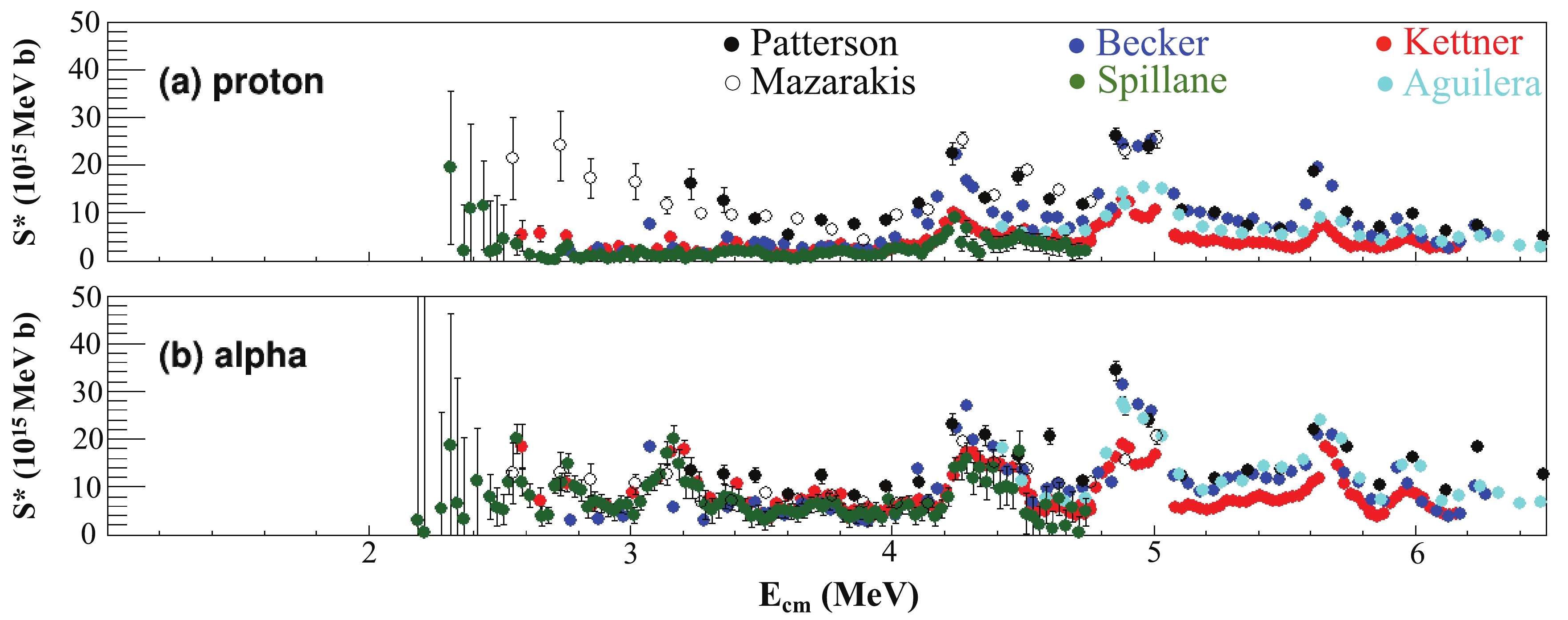Figure2. (color online ) S^* factor of measured cross sections for the p and $ \alpha $ channels, respectively. S^* factors measured by Kettner et al. (red solid circle), Aguilera et al. (cyan solid circle), and Spillane et al. (green solid circle) are based on the characteristic $ \gamma $-ray technique. S^* factors measured by Becker et al. (blue solid circle), Patterson et al. (black solid circle), and Mazarakis et al. (black open circle) are based on particle spectroscopy data.

Figure3. (color online) Ratios of various data sets as shown in Fig. 2 to the baseline data set, representing the measurement by Kettner et al. The means and errors of the baseline data sets are interpolated in the calculations of ratios. The shaded areas shown in the ratio plots correspond to a deviation of ±30%.

Differences exist also among the S^* factors obtained using the same experimental techniques. Taking particle spectroscopy data as an example, the summed S^* factors of the proton channel of Becker et al., Patterson et al., and Mazarakis et al. are in agreement within ±20% for $ E_{\rm cm}> $4 MeV. However, the S^* factors of the data set of Becker et al. are lower than those of the other two data sets by a factor of up to 10 when the energies are below 3.4 MeV. The difference at high energies may be explained by the normalization uncertainties, such as target thickness and/or beam intensity. The difference at lower energies, in contrast, mainly comes from the fact that Becker et al. measured a lower number of channels than the other two groups. Aguilera et al., Spillane et al., and Kettner et al. all used the characteristic $ \gamma $-rays to measure the S^* factors. Compared to the S^* factors of Kettner et al., the S^* factors of Agulera et al. are approximately 30% higher, while those of Spillane et al. are lower by more than 30%–60%. The only significant difference in the experimental procedure of these three studies is that Aguilera et al. placed the Ge detector at 55° to minimize the effect of the $ \gamma $-ray angular distribution, while the other two groups chose 0° as their detection angle. The difference between the results of Spillane et al. and Ketter et al. shows that this effect of angular distribution is below 30%.
Measures have been taken in some experiments to account for the missing channels to obtain the actual total S^* factor. For example, Becker et al. summed all the observed particle channels to obtain the total fusion cross sections. In cases where the data for a given particle group were only available over a limited energy range, the energy-averaged S^* factors of these groups were extrapolated down to the threshold and added to the total S^* factors. Based on the result of Becker et al., Spillane et al. estimated the mean values of the ratios of the 440 keV line to the sum of all the proton channels and the 1634 keV line to the sum of all the alpha channels to be 0.55 ± 0.05 and 0.48 ± 0.05, respectively. This correction is included in their reported S^* factors of the proton and alpha channels. Aguilera et al. took a different approach by adding the S^* factors of the $ p_0 $ and $ \alpha_0 $ channels to their measured S^* factors of the 440 and 1634 keV $ \gamma $-rays to obtain the total S^* factors. Using their own data set as the standard, Aguilera et al. shifted the energies and adjusted the normalization factors to bring a reasonable agreement among the existing experimental results.
In this paper, we introduce a novel approach based on the statistical model to predict the branching ratio of each decay channel. The prediction is validated by the experimental data obtained by particle spectroscopy. The branching ratios are predicted for each experiment and used to convert the observed S^* factors into the total S^* factor of ¹²C+¹²C.

The spin populations of the ²⁴Mg compound nucleus are calculated by fitting the average S^* factor of ¹²C+¹²C with a simple powered Woods-Saxon potential. The fusion cross sections are calculated by the CCFull code [27]. The corresponding spin populations of the ²⁴Mg compound nucleus are shown in Fig. 4. Only even spins with positive parity are allowed, as the ¹²C+¹²C system is composed of two identical bosons. The calculation shows that the spin of the compound nucleus is dominated by the 2⁺ and 0⁺ states at energies below $ E_{\rm cm} $=3 MeV. Theoretical calculations show that some spins could be enhanced at certain energies by the molecular resonances in the entrance channel. The smooth spin population shown here, however, only represents average behavior.
Figure4. (color online) Spin populations of the ²⁴Mg compound nucleus produced by ¹²C+¹²C fusion, calculated with CCFull code [27]. Dominant components have spins $ 0^+ $, $ 2^+ $, $ 4^+ $ and $ 6^+ $.

The fusion evaporation cross sections for different decay channels are modeled with the Hauser-Feshbach formula [28, 29]. Let all quantum numbers that specify the entrance and exit channels be denoted by $ \alpha $ and $ \alpha^\prime $, respectively. Similarly, l + S = J = l’ + S’, S = I + i, and S’ = I’ + i’ denote the angular momentum coupling for orbital angular momentum l ($ l^\prime $), channel spin S ($ S^\prime $), total angular momentum J, and intrinsic angular momenta I ($ I^\prime $) and i ($ i^\prime $) [30]. The Hauser-Feshbach formula is expressed as

$ \sigma_{\alpha\alpha'} = \pi\lambda\bar{\; \; }_\alpha^2\sum_J\frac{2J+1}{(2I+1)(2i+1)}\frac{[\Sigma_{Sl}T_l(\alpha)]^J[\Sigma_{S'l'}T_l(\alpha')]^J}{[\Sigma_{a'',S''l''}T_{l''}(\alpha'')]^J} $

(2)

for the angle integrated cross section, where $ T_l $ denotes the optical model transmission coefficient.
The decay of the carbon-fusion-made ²⁴Mg compound nucleus with a given spin (0, 2, 4, or 6) is calculated using the statistical model code, Talys [31]. The numbers of experimentally known states considered in the present calculation are 50 for ²³Na, 13 for ²⁰Ne, and 20 for ²³Mg. The default level density and global optical model are used above the limit of the experimentally known states. After being weighted by the predicted spin population of the ²⁴Mg compound nucleus shown in Fig. 4, the branching ratios of each $ \alpha $- and p- evaporation channel are derived and plotted, as shown in Fig. 5. The branching ratios for highly excited states of both channels fall rapidly with decreasing energy. In the $ \alpha $-channel, the ground ($ \alpha_0 $) and first excited ($ \alpha_1 $) states dominate the total $ \alpha $ evaporation cross sections for $ E_{\rm cm} < $3 MeV. However, in the p-channel, the situation is more complicated: in addition to the ground ($ p_0 $) and first excited ($ p_1 $) states, the $ p_{2,3,4,5,6,7,8,9} $ states considerably contribute to the total proton evaporation cross sections.
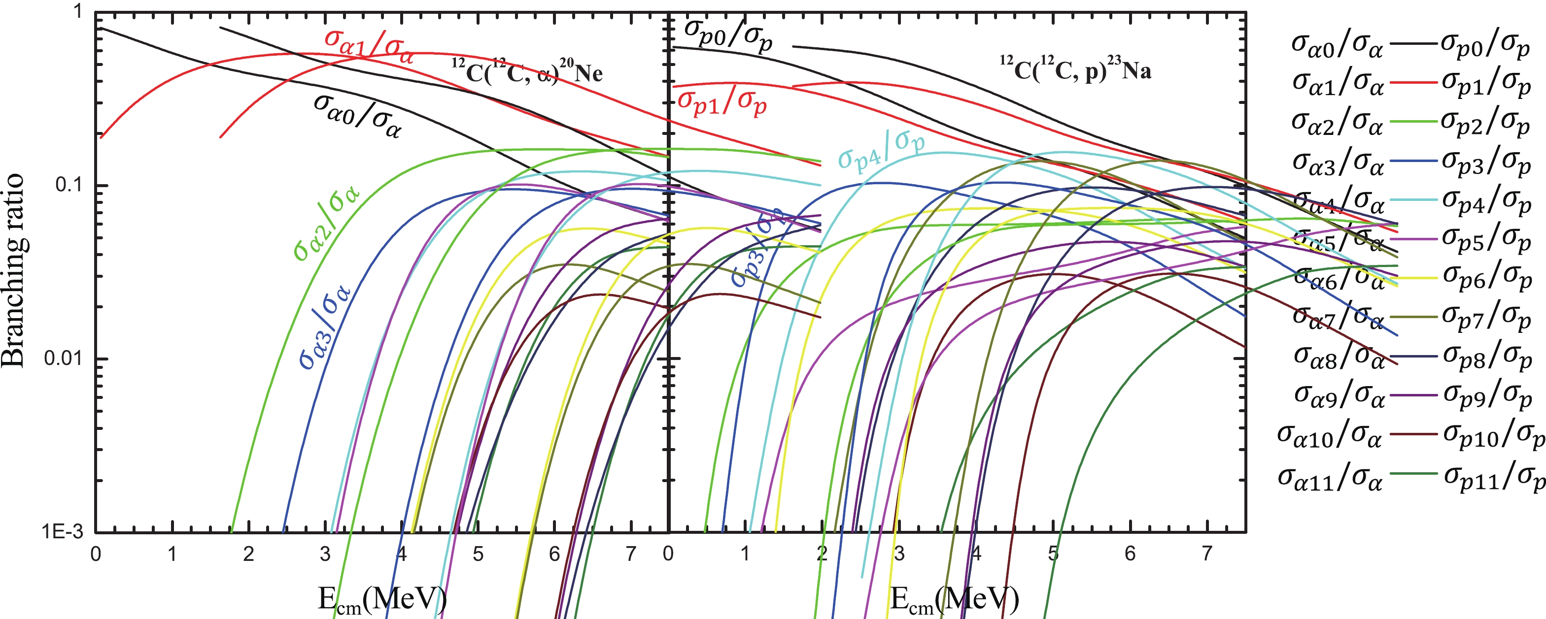Figure5. (color online) Branching ratios, calculated using Talys [31], for each state ($ \alpha_{i} $, $ p_{i} $, distinguished by colors, where i = 0, 1, 2,...,11) of the $ \alpha $ particle and proton evaporation channels in the ¹²C+¹²C fusion reaction.

The calculated branching ratios are compared with the experimental values obtained by Becker et al. [10], who reported information on numerous separated states in both $ \alpha $- and p- channels, including $ \alpha_0 $, $ \alpha_1 $, $ \alpha_2 $, $ \alpha_3 $, $ \alpha_4 $, $ \alpha_5 $, $ \alpha_6 $, $ \alpha_7 $, $ \alpha_8 $+$ \alpha_9 $, $ \alpha_{10} $, $ \alpha_{11} $, $ \alpha_{12} $ and $ p_0 $, $ p_1 $, $ p_2 $, $ p_3 $, $ p_4 $+$ p_5 $, $ p_6 $, $ p_7 $, $ p_8 $+$ p_9 $, $ p_{10} $, $ p_{11} $, $ p_{12} $, $ p_{13} $, $ p_{14} $+$ p_{15} $+$ p_{16} $. The $ \sigma_{p_0} $/$ \sigma_{p} $, $ \sigma_{p_1} $/$ \sigma_{p} $, ($ \sigma_{p_0}+\sigma_{p_1} $)/$ \sigma_{p} $, and $ \sum_{i = 0}^5\sigma_{p_i} $/$ \sigma_{p} $ ratios of the present calculation are displayed with the experimental data of Becker et al. [10] on the left side of Fig. 6. Similarly, the $ \sigma_{\alpha_0} $/$ \sigma_{\alpha} $, $ \sigma_{\alpha_1} $/$ \sigma_{\alpha} $, ($ \sigma_{\alpha_0}+\sigma_{\alpha_1} $)/$ \sigma_{\alpha} $, and $ \sum_{i = 0}^3\sigma_{\alpha_i} $/$ \sigma_{\alpha} $ ratios are displayed with the corresponding experimental data on the left side of Fig. 7. To compare the theoretical calculation of Talys with the actual particle measurement, we take the experimental cut-off energy for each observed state of Becker et al. [10] into account. The calculations of the branching ratios without considering the cut-off energy are shown as solid lines and labeled Theory1. In reality, the most highly excited fusion residues are accompanied by very low energy protons and $ \alpha $ particles that could not be sensed by the experimental particle detectors and thus were missed in the measurements. These cut-off energies have been included in a second set of calculations, shown as dashed lines and labeled Theory2. The difference between Theory1 (ideal) and Theory2 (reality) arising from the missing channels is related to the detection threshold and/or background in the particle measurements. They are nearly the same for all energies in the relevant $ \alpha $-channels and for E_cm>3.4 MeV in p-channels.
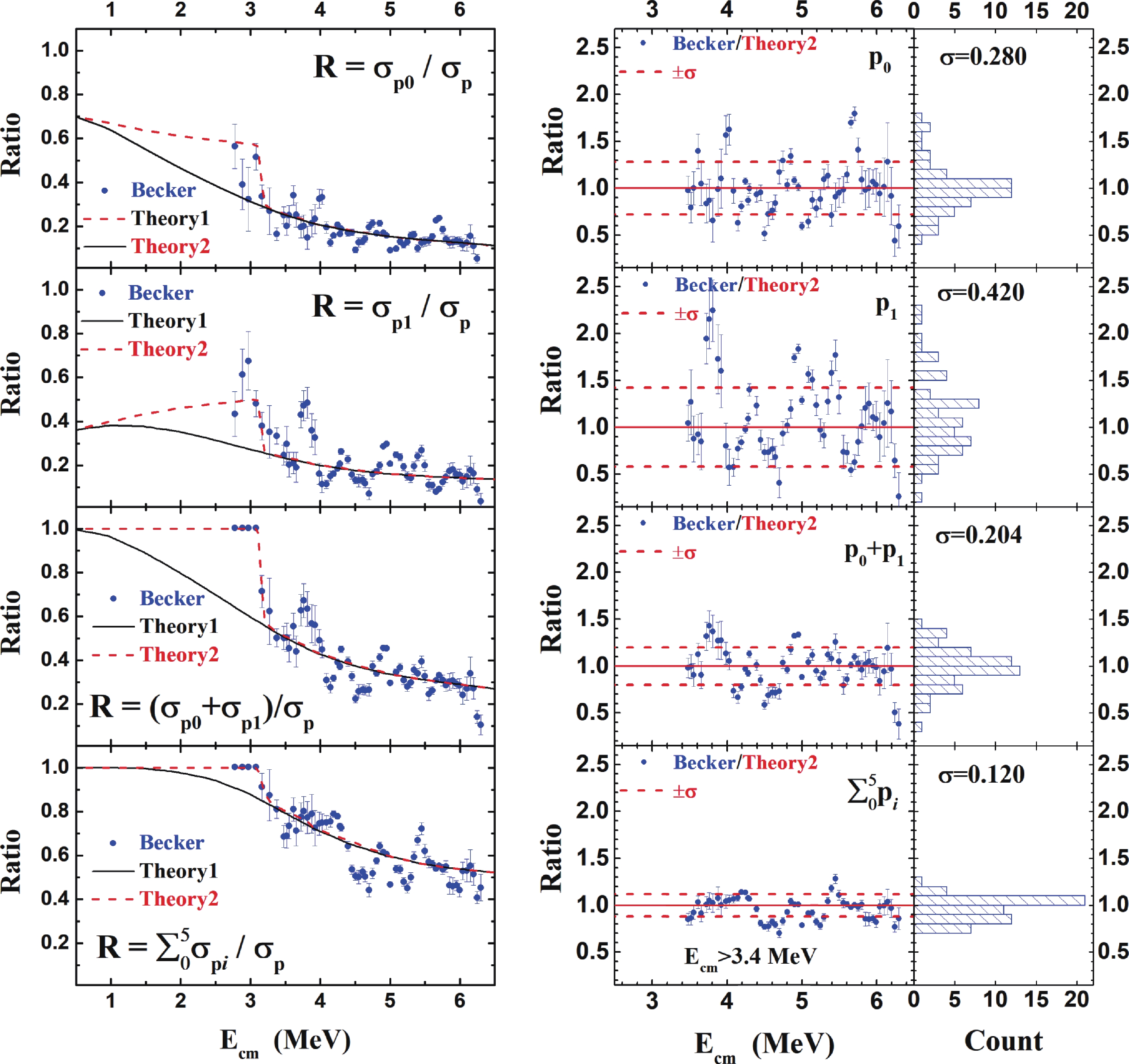Figure6. (color online) Comparison of theoretical branching ratios with those of experimental data [10] for the p-channel. (left) The calculated $ \sigma_{p_0} $/$ \sigma_{p} $, $ \sigma_{p_1} $/$ \sigma_{p} $, ($ \sigma_{p_0}+\sigma_{p_1} $)/$ \sigma_{p} $, and $ \sum_{i = 0}^5\sigma_{p_i} $/$ \sigma_{p} $ ratios are depicted with experimental data from Becker et al. [10]. Theory1 is the present calculation by Talys, while Theory2 takes into account the lack of experimental sensitivity to protons with energies below a certain cut-off value (see text for details). (right) Values of Becker/Theory2 for branching ratios shown on the left are calculated and displayed. Relevant statistics for each distribution are also displayed, showing the average value (Mean = 1) and standard deviation ($ \sigma $).

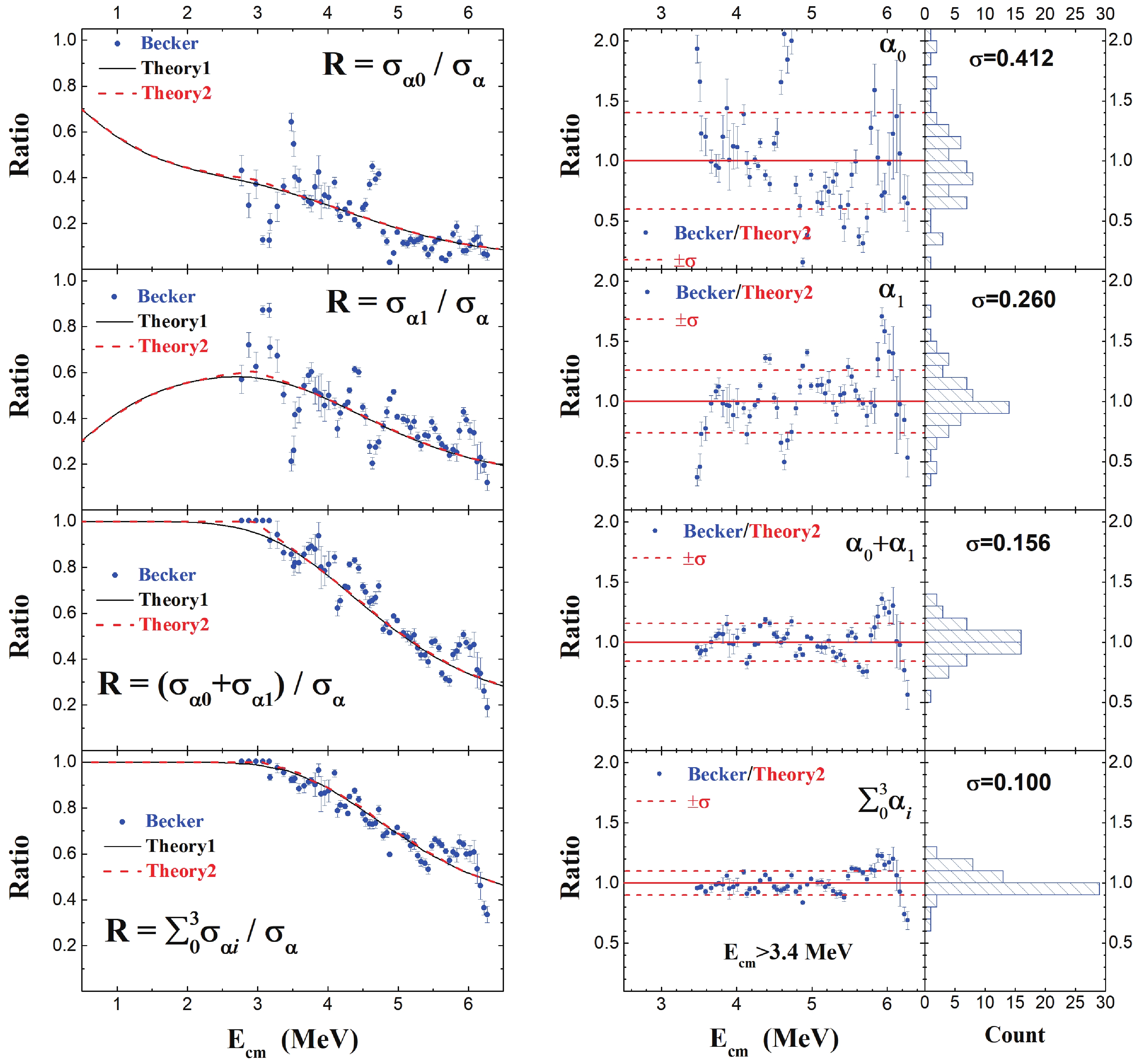Figure7. (color online) Comparison of theoretical branching ratios with those of experimental data [10] for the $ \alpha $-channel. (left ) The calculated $ \sigma_{\alpha_0} $/$ \sigma_{\alpha} $, $ \sigma_{\alpha_1} $/$ \sigma_{\alpha} $, ($ \sigma_{\alpha_0}+\sigma_{\alpha_1} $)/$ \sigma_{\alpha} $, and $ \sum_{i = 0}^3\sigma_{\alpha_i} $/$ \sigma_{\alpha} $ ratios are depicted with experimental data from Becker et al. [10]. Theory1 is the present calculation by Talys, while Theory2 takes into account the lack of experimental sensitivity to alphas with energies below a certain cut-off value (see text for details). (right) Values of Becker/Theory2 for the branching ratios shown on the left are calculated and displayed. Relevant statistics for each distribution are also displayed, showing the average value (Mean = 1) and standard deviation ($ \sigma $).

The present calculations (Theory 1 and Theory 2) describe a smoothly averaged trend for the experimental branching ratios obtained from Becker's data [10]. The contribution of the ground state is approximately 40% for $ \sigma_{\alpha_0} $and 30% for $ \sigma_{p_0} $ at $ E_{\rm cm} $ = 3 MeV. The branching ratios for $ \sigma_{p_0}+\sigma_{p_1} $ and $ \sigma_{\alpha_0}+\sigma_{\alpha_1} $ are larger than 50% and 90% at $ E_{\rm cm} $ = 3 MeV, respectively, and continuously increase with decreasing energy. There are significant fluctuations in the $ p_0 $, $ p_1 $, $ \alpha_0 $, and $ \alpha_1 $ channels due to strong resonances.
To compare trends of the branching ratios obtained from the particle spectroscopy measurement with the theoretical prediction, the values of Becker/Theory2 are calculated by dividing the experimental ratios by the theoretical predictions and displayed on the right side of Fig. 6 and Fig. 7. Each theoretical ratio has been tuned using a renormalization factor, f, to achieve the best fit. For cases where the numerator in the ratio is also part of the denominator, such as $ p_0 $/$ p_{\rm tot} $, the scaled ratio is provided by the numerator/(numerator+f (denominator-numerator)). Otherwise, f is applied directly to the ratio. The applied values of f ranged from 0.7 to 1.3.
The statistical distribution of Becker/Theory2 for each branching ratio is analyzed in the energy range above 3.4 MeV to avoid the influence of missing channels. The distribution widths, which represent the fluctuation of the experimental values around the predictions, are summarized in Table 2. The distribution widths of the Becker/Theory2 ratios are approximately 30% (1$ \sigma $) in the $ p_0 $, $ p_1 $, $ \alpha_0 $, and $ \alpha_1 $ channels. Interestingly, the fluctuations of data around the theoretical values decrease as the branching ratios of the protons and $ \alpha $channels increase. In the p-channel, for example, the branching ratio of $ \sum_{i = 0}^5\sigma_{p_i} $/$ \sigma_{p} $ is approximately 50% to 70% between 3.5 MeV$ <E_{\rm cm}< $6.5 MeV. The fluctuation for $ \sum_{i = 0}^5\sigma_{p_i} $ is approximately ±12% (1$ \sigma $), in contrast to the 30% to 50% (1$ \sigma $) fluctuation observed in the $ p_0 $ and $ p_1 $ channels. A strong resonance is observed around $ E_{\rm cm} = $3.8 MeV in the summation of $ p_0 $ and $ p_1 $; however, it disappears when more proton channels are summed up to $ p_5 $. As we increase the branching ratio of the observed proton channels, the fluctuation incurred by the resonance feature of the ¹²C+¹²C channel also becomes lower. In the $ \alpha $-channel, the branching ratio of $ \sum_{i = 0}^3\sigma_{\alpha_i} $/$ \alpha $ is between 50% and 100% in the range 3.5 MeV$ <E_{\rm cm}< $6.5 MeV. The fluctuation for $ \sum_{i = 0}^3\sigma_{\alpha_i} $ is approximately ±14%(1$ \sigma $), in contrast to the one higher than 30% (1$ \sigma) $ observed in $ \alpha_0 $ and $ \alpha_1 $. This fluctuation is expected to decrease, considering that the ratio ($ \sigma_{\alpha_0}+\sigma_{\alpha_1} $)/$ \alpha $ reaches almost 100% for $ {E}_{\rm cm}< $3.5 MeV.

Ratio	Value at 4 MeV	Relative fluctuation (1$\sigma$)
$\sigma_{p_0}$/$\sigma_p$	0.21	28%
$\sigma_{p_1}$/$\sigma_p$	0.21	42%
($\sigma_{p_0}$+$\sigma_{p_1}$)/$\sigma_p$	0.42	20%
$\sum_{i=0}^5\sigma_{p_i}$/$\sigma_p$	0.71	12%
$\sigma_{\gamma(440)}$/$\sigma_p$	0.48	14%
[$\sigma_{p_0}+\sigma_{\gamma(440)}$]/$\sigma_p$	0.69	8%
$\begin{aligned}[{\sigma _{{p_0}}} + {\sigma _{\gamma (440)}} + {\sigma _{\gamma (2391)}} \\+ {\sigma _{\gamma (2640)}} + {\sigma _{\gamma (2982)}}]/\sigma_p\end{aligned}$	0.93	3%
$\sigma_{\alpha_0}$/$\sigma_{\alpha}$	0.24	41%
$\sigma_{\alpha_1}$/$\sigma_{\alpha}$	0.5	26%
($\sigma_{\alpha_0}$+$\sigma_{\alpha_1}$)/$\sigma_{\alpha}$	0.74	16%
$\sum_{i=0}^3\sigma_{\alpha_i}$/$\sigma_{\alpha}$	0.89	10%
$\sigma_{\gamma(1634)}$/$\sigma_{\alpha}$	0.67	16%
[$\sigma_{\alpha_0}+\sigma_{\gamma(1634)}$]/$\sigma_{\alpha}$	0.94	7%

Table2.Theoretical branching ratios at 4 MeV and their relative fluctuations in the range of 3.4 to 6 MeV.

It has been reported in ¹²C(¹³C,p)²⁴Na that the average branching ratio is approximately 0.25 with a relative fluctuation of 14% (1$ \sigma $) [32]. However, to reach a relative fluctuation as low as 14% in ¹²C+¹²C, the branching ratio must be above 0.5 for the proton channel and 0.7 for the $ \alpha $ channel, as listed in Table 2. This disparity may arise from significant differences in the compound nuclei, ²⁴Mg and ²⁵Mg [17]. Compared to ¹²C+¹³C, the lower level density in the ¹²C+¹²C entrance and exit channels indicates that the nuclear structure plays a more significant role, which results in larger fluctuations in the branching ratio.

We use the statistical model result to estimate the branching ratios of the characteristic $ \gamma $ rays, e.g., 1634, 4967, and 5621 keV for the $ \alpha $-channel and 440, 2076, 2391, 2640, 2982, and 3848 keV for the p-channel. The cross sections for the production of these characteristic $ \gamma $ rays, which directly transit to the ground state ($ \alpha_0 $ or $ p_0 $), are given by the expression

$ \sigma_\gamma = \sum_i f_i\sigma_i, $

(3)

where $ \sigma_i $ are the partial cross sections for the $ i^{\rm th} $ excited state in the residual nucleus, and $ f_i $ represents the transit factors, whose values are listed in Tables 3 and 4 for $ \alpha $- and p- evaporation channels, respectively. They are deduced based on the $ \gamma $ transition branching ratios from NNDC [33].

	$\sigma_{\gamma(1634)}$	$\sigma_{\gamma(4967)}$	$\sigma_{\gamma(5621)}$
$\sigma_{\alpha_1}$	100
$\sigma_{\alpha_2}$	100
$\sigma_{\alpha_3}$	99.4	0.6
$\sigma_{\alpha_4}$	6.47	0.002	0.53
$\sigma_{\alpha_8}$	76.6	0.07	0.13
$\cdots$	$\cdots$	$\cdots$	$\cdots$

Table3.Numerical factors (%) for yields of characteristic $\gamma$-rays from partial cross sections of $\alpha$-evaporation channels.

	$\sigma_{\gamma(440)}$	$\sigma_{\gamma(2076)}$	$\sigma_{\gamma(2391)}$	$\sigma_{\gamma(2640)}$	$\sigma_{\gamma(2982)}$	$\sigma_{\gamma(3848)}$
$\sigma_{p_1}$	100
$\sigma_{p_2}$	91.8	8.2
$\sigma_{p_3}$	34.3		65.7
$\sigma_{p_4}$				100
$\sigma_{p_5}$	97.1	2.9
$\sigma_{p_6}$	41.2		0.2		58.6
$\sigma_{p_7}$	79.4		0.9	19.5	0.3
$\sigma_{p_8}$	66.4	5.0	0.004	4.5	1.2	22.9
$\sigma_{p_9}$	17.7	0.7	0.7		1.35
$\sigma_{p_{10}}$	2.8		0.7
$\sigma_{p_{11}}$	97.4	2.6
$\sigma_{p_{12}}$	80.9	1.8	0.01		4.2
$\sigma_{p_{13}}$	96.0	4.0
$\sigma_{p_{14}}$	29.1
$\sigma_{p_{15}}$	43.1	0.08		4.5	0.02	0.3
$\sigma_{p_{16}}$	67.1		32.9
$\vdots$	$\vdots$	$\vdots$	$\vdots$	$\vdots$	$\vdots$	$\vdots$

Table4.Numerical factors (%) for yields of characteristic $\gamma$-rays from partial cross sections of proton-evaporation channels.

The theoretical branching ratios of $ \sigma_{\gamma(1634)} $/$ \sigma_\alpha $ and $ \sigma_{\gamma(440)} $/$ \sigma_p $ are listed in Table 5. Notably, the 1634 keV transition of ²⁰Ne is mixed with the 1636 transition of ²³Na. $ \gamma $-spectroscopy cannot resolve these two $ \gamma $-rays owing to Doppler broadening. This contribution can be estimated based on the observed yield of the 440 keV transition from ²³Na and the predicted ratio of $ \sigma_{\gamma(1636)} $/$ \sigma_{\gamma(440)} $.

$ E_{\rm cm} $	$ \sigma_{p_0} $/$ \sigma_p $	$ \sigma_{\gamma(440)} $/$ \sigma_p $	$ \sigma_{\alpha_0} $/$ \sigma_\alpha $	$ \sigma_{\gamma(1634)} $/$ \sigma_\alpha $	$ \sigma_{\gamma(1636)} $/$ \sigma_{\gamma(440)} $
0.5	0.6986	0.3432	0.6798	0.3260	0.0063
0.6	0.6868	0.3518	0.6570	0.3490	0.0112
0.8	0.6638	0.3683	0.6104	0.3960	0.0201
1	0.6378	0.3847	0.5665	0.4400	0.0288
1.2	0.6025	0.3988	0.5336	0.4731	0.0392
1.4	0.5673	0.4125	0.5016	0.5051	0.0489
1.5	0.5494	0.4181	0.4879	0.5187	0.0536
1.6	0.5322	0.4214	0.4777	0.5290	0.0587
1.8	0.4977	0.4277	0.4572	0.5494	0.0687
2	0.4640	0.4323	0.4383	0.5683	0.0786
2.2	0.4321	0.4336	0.4234	0.5831	0.0890
2.4	0.4005	0.4344	0.4091	0.5973	0.0996
2.5	0.3851	0.4357	0.4022	0.6040	0.1051
2.6	0.3700	0.4374	0.3953	0.6108	0.1108
2.8	0.3408	0.4400	0.3814	0.6242	0.1224
3	0.3120	0.4452	0.3672	0.6370	0.1338
3.2	0.2867	0.4523	0.3522	0.6482	0.1455
3.4	0.2613	0.4593	0.3369	0.6597	0.1567
3.5	0.2508	0.4630	0.3289	0.6626	0.1624
3.6	0.2412	0.4670	0.3198	0.6642	0.1676
3.8	0.2219	0.4750	0.3015	0.6678	0.1780
4	0.2048	0.4826	0.2832	0.6664	0.1877
4.2	0.1922	0.4870	0.2621	0.6570	0.1968
4.4	0.1793	0.4927	0.2420	0.6465	0.2049
4.5	0.1743	0.4937	0.2310	0.6397	0.2089
4.6	0.1696	0.4940	0.2208	0.6308	0.2127
4.8	0.1608	0.4958	0.2003	0.6136	0.2194
5	0.1527	0.4962	0.1810	0.5952	0.2267
5.2	0.1465	0.4955	0.1637	0.5756	0.2339
5.4	0.1400	0.4954	0.1454	0.5568	0.2410
5.5	0.1374	0.4952	0.1387	0.5477	0.2454
5.6	0.1351	0.4948	0.1325	0.5389	0.2505
5.8	0.1299	0.4946	0.1196	0.5219	0.2606
6	0.1250	0.4950	0.1086	0.5066	0.2714
6.2	0.1202	0.4966	0.1003	0.4952	0.2830
6.4	0.1149	0.4982	0.0920	0.4842	0.2957
6.5	0.1120	0.4991	0.0878	0.4785	0.3024

Table5.Theoretical branching ratios predicted by the statistical model.

The statistical model calculation provides branching ratios to convert the observed particle or characteristic $ \gamma $-ray S^* factors into the S^* factors of ¹²C(¹²C,p)²³Na and ¹²C(¹²C,p)²³Na. Two principles are followed to reduce the systematic error of the statistical model. First, the total S^* factor of the proton (alpha) channel is only calculated from the corresponding S^* factors observed by particle spectroscopy or characteristic-$ \gamma $ rays to minimize the influences incurred by the mismatched optical potentials of the p and $ \alpha $ channels. Second, all possible observed channels are included, which increases the branching ratio and results in less systematic fluctuations.
For measurements using the characteristic $ \gamma $-ray method, we add the ground state transitions ¹²C(¹²C,$ p_0 $)²³Na and ¹²C(¹²C,$ \alpha_0 $)²⁰Ne obtained with particle spectroscopy to the observed $ \gamma $-ray S^* factors. The theoretical and experimental branching ratios are shown in Fig. 8 and Fig. 9. The inclusion of the ground state channels ($ p_0 $,$ \alpha_0 $) is important, especially for $ E_{\rm cm}< $3.5 MeV, because these ground state channels are expected to contribute significantly, as shown in Fig. 6 and Fig. 7. For the $ \alpha $ channel, the sum of $ \sigma_{\alpha 0} $ and $ \sigma_{\gamma(1634)} $ contributes approximately 60% ~ 90% of the ¹²C(¹²C,$ \alpha $)²⁰Ne cross sections at 3.4 ~ 6.0 MeV in the center of mass frame. The fluctuation of the experimental [$ \sigma_{\alpha_0} $ + $ \sigma_{\gamma(1634)} $]/$ \sigma_{\alpha} $ around the predicted ratio reflects the systematic error of the latter, which is estimated to be 7.2% based on the experimental data in the energy range from 3.4 to 6.0 MeV. The fluctuation is expected to be smaller and eventually vanish at stellar energies, as the summation becomes equal to the total cross sections of ¹²C(¹²C,$ \alpha $)²⁰Ne at these energies. Therefore, only measuring these two components is sufficient for determining the ¹²C(¹²C,$ \alpha $)²⁰Ne S^* factor in the important energy range. The proton channel is slightly more complicated. The sum of $ \sigma_{p_0} $ and $ \sigma_{\gamma(440)} $ contributes nearly 70% of the ¹²C(¹²C,p)²³Na S^* factor at $ E_{\rm cm} $ = 4 MeV. The systematic error of the theoretical [$ \sigma_{p_0} $ + $ \sigma_{\gamma(440)} $] / $ \sigma_{p} $ ratio is estimated to be 8.2%. As the ratio of [$ \sigma_{p_0} $ + $ \sigma_{\gamma(440)} $] / $ \sigma_{p} $ increases from 70% ~ 90% at astrophysical energies, the systematic uncertainty is expected to decrease. By including further transitions, such as 2391, 2640, and 2982 keV of ²³Na, the ratio of the sum of these observable channels to ¹²C(¹²C,p)²³Na becomes more than 90% at all energies, as shown in Fig. 9, and the systematic error is less than 3%, which is mainly limited by the experimental uncertainty of the branching ratio.
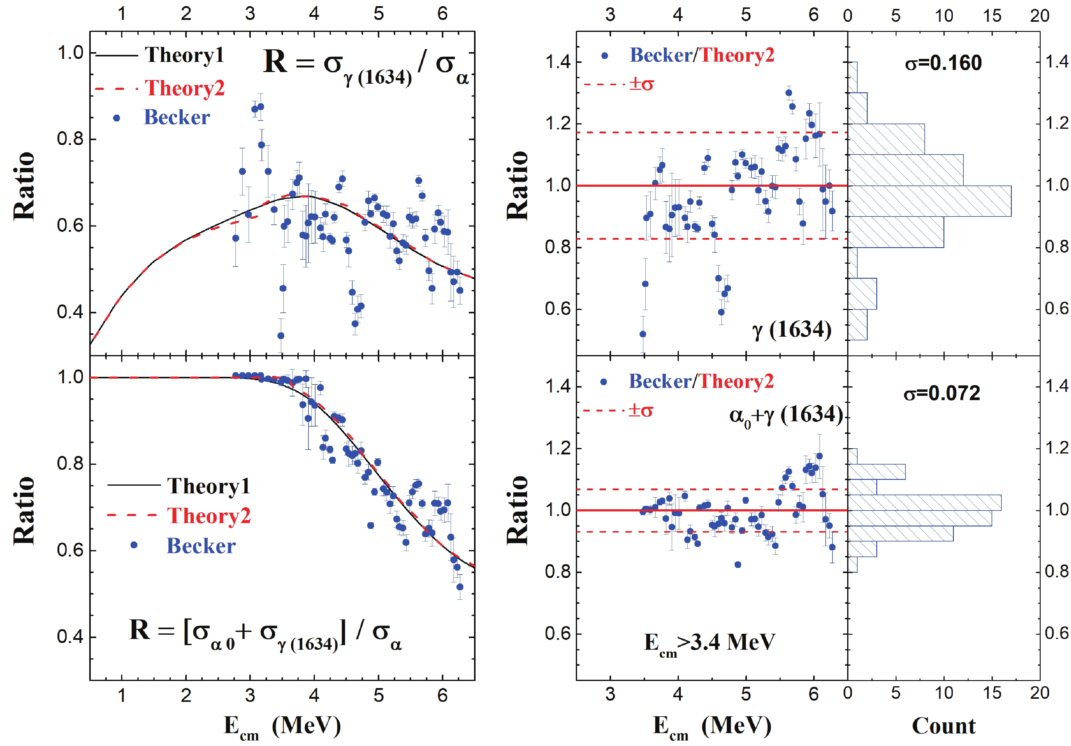Figure8. (color online) Comparison of branching ratios calculated with experimental data measured by Becker et al. [10] for $ \alpha_0 $ and the 1634 keV characteristic $ \gamma $ ray. (left) The $ \sigma_{\gamma(1634)} $/$ \sigma_{\alpha} $ and [$ \sigma_{\alpha_0} $ + $ \sigma_{\gamma(1634)} $]/$ \sigma_{\alpha} $ ratios are shown. Theory1 is the present calculation by Talys, while Theory2 takes into account the experimental cut-off energies of Becker et al. [10], as discussed in the text. (right) Values of Becker/Theory2 for the ratios shown on the left are calculated and displayed. Relevant statistics are also shown with average value (Mean = 1) and standard deviation ($ \sigma $).

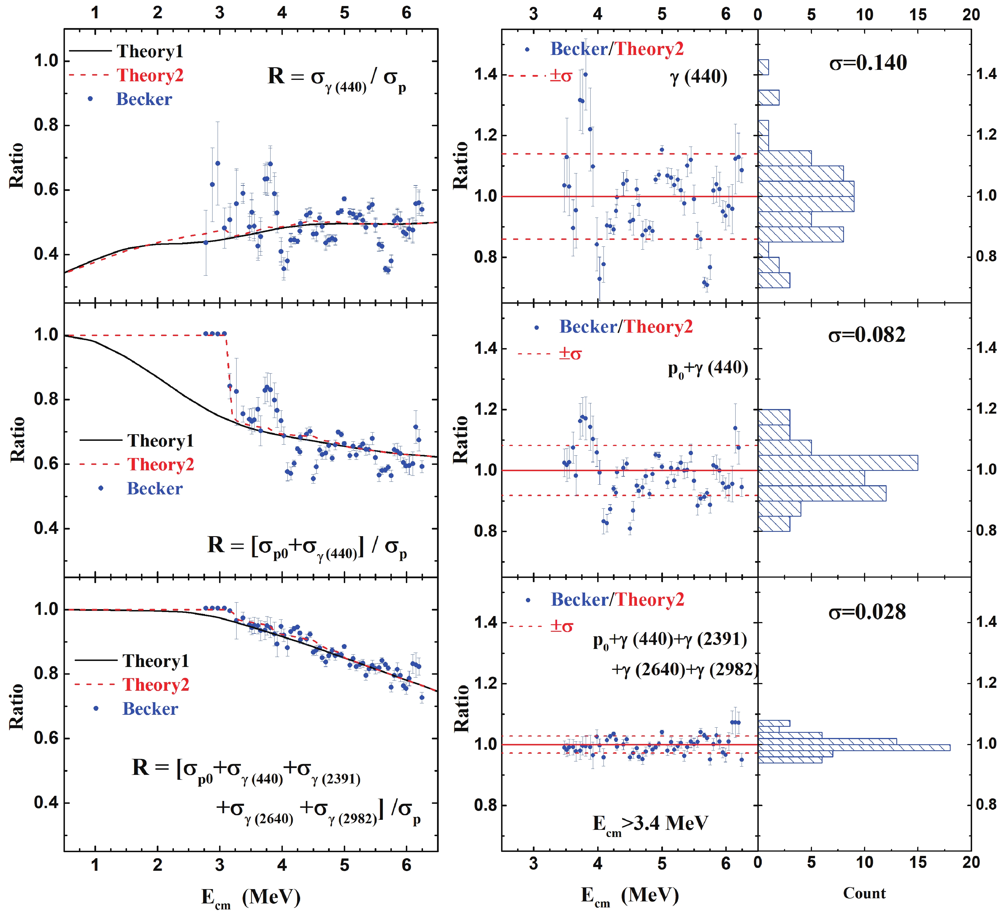Figure9. (color online) Comparison of branching ratios calculated with experimental data measured by Becker et al. [10] for $ p_0 $and 440 keV characteristic and other $ \gamma $ rays. (left) The $ \sigma_{\gamma(440)} $ / $ \sigma_{p} $, [$ \sigma_{p_0} $ + $ \sigma_{\gamma(440)} $] / $ \sigma_{p} $, and [$ \sigma_{p_0} $ + $ \sigma_{\gamma(440)} $ + $ \sigma_{\gamma(2391)} $ + $ \sigma_{\gamma(2640)} $ + $ \sigma_{\gamma(2982)} $] / $ \sigma_{p} $ ratios are shown. Theory1 is the present calculation by Talys, Theory2 takes into account the experimental cut-off energies of Becker et al. [10], as discussed in the text. (right) Values of Becker/Theory2 for the ratios shown on the left are calculated and displayed. The relevant statistics are also shown with the average value (Mean = 1) and standard deviation ($ \sigma $).

The total p- and $ \alpha $- S^*(E) factors from charged-particle measurements of Patterson et al. [6], Mazarakis and Stephens [9], and Becker et al. [10] are shown in Fig. 10. The data obtained by Becker et al. were corrected to account for the missing channels by applying the ratios shown in Fig. 6 and Fig. 7. The data of Mazarakis et al. [9] and Kettner et al. [34] were shifted by 100 keV and 30 keV, respectively, to match the resonances measured by Aguilera et al. [15] and Spillane et al. [16].
Figure10. (color online) S^* factor of the proton, alpha, and neutron channels and the sum of the three channels after correcting for missing channels.

Based on the ground state data from Becker et al. [10] and the calculated ratios for [$ \sigma_{\alpha 0} $ + $ \sigma_{\gamma(1634)} $]/$ \sigma_{\alpha} $ and [$ \sigma_{p0} $ + $ \sigma_{\gamma(440)} $] / $ \sigma_{p} $ (Figs. 8 and 9), the data of Kettner et al. [34], Aguilera et al. [15] and Spillane et al. [16] have been corrected.
Using the data of Kettner et al. [14] as the baseline, the ratios of the S^* factors of the proton and alpha channels and the total S^* factors are computed for each data set and shown in Fig. 11.
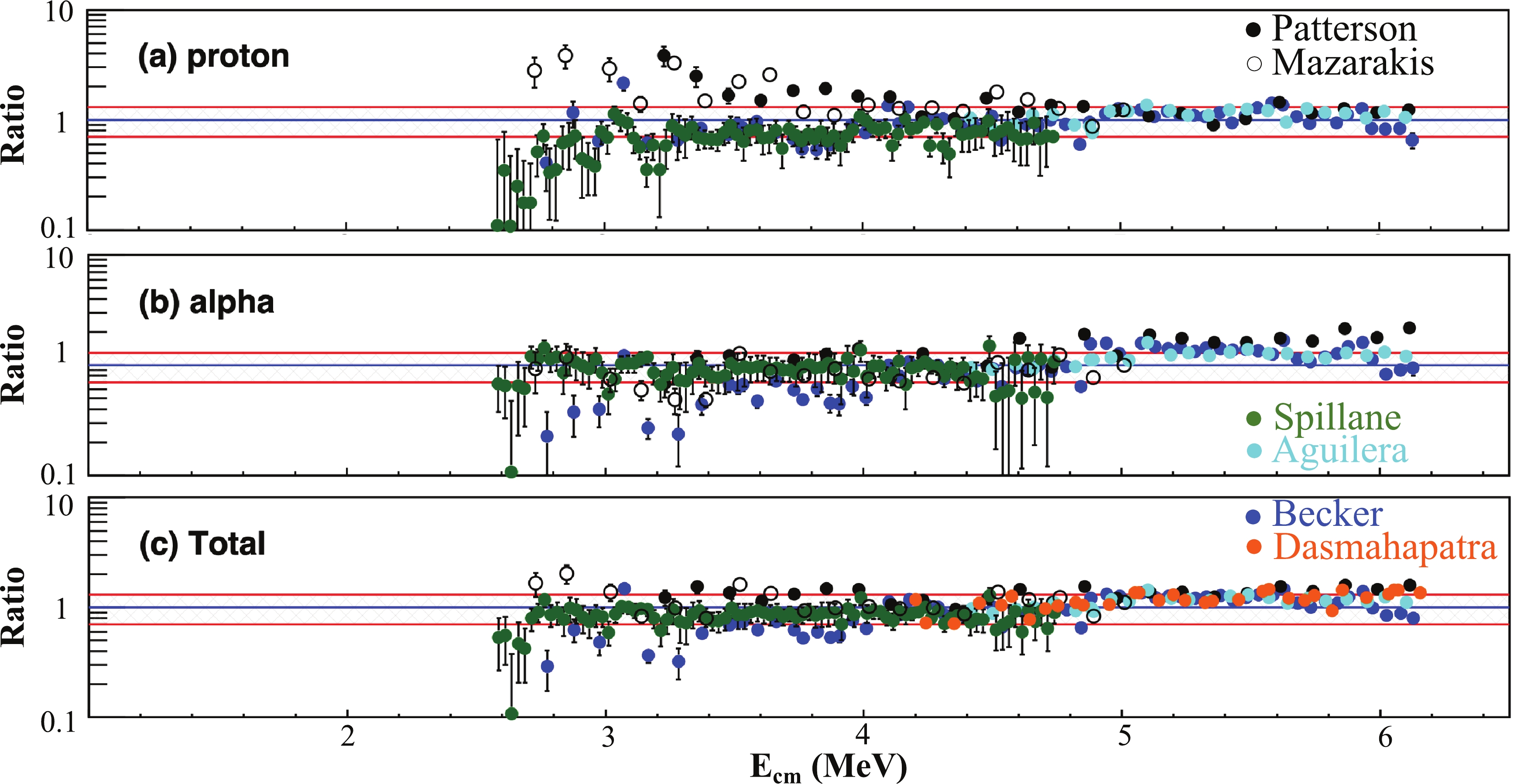Figure11. (color online) Ratios of various S^* factors to baseline S^* factors, measured by Kettner et al. after correcting for missing channels. The means and errors of the baseline data sets are interpolated in the calculations of ratios. The shaded areas shown in the ratio plots correspond to ±30% deviations.

For the proton channel, the S^* factors obtained with $ \gamma $-spectroscopy (Spillane, Aguilera and Kettner) match the S^* factors obtained with particle-spectroscopy (Becker, Patterson and Mazarakis) within ± 30% deviations at energies above 4 MeV. This observation indicates the importance and effectiveness of the correction done in the current study. Some systematic deviations are observed in the range of 5 to 6 MeV, possibly arising from systematic errors in some of the experiments, which might be improved in the future. At energies below 4 MeV, the result of Spillane is approximately 20%-30% lower than the baseline data (Kettner). Because both experiments were conducted with $ \gamma $-ray spectroscopy and corrected by the same branching ratio, this difference can only arise from experimental systematic errors. The three particle spectroscopy experimental results of Becker, Patterson, and Mazarakis, disagree at energies below 4.2 MeV. The results obtained from the measurements of Patterson and Mazarakis are almost a factor of four higher than the result obtained from the measurement of Becker. Nevertheless, the S^* factor of Spillane agrees with the one from Becker even though these two measurements were performed using different methods. It is well known that the deuterium impurity in carbon targets may contribute a background in the proton spectrum via the d(¹²C,p)¹³C reaction. Because the measurement of 440 keV is less affected by the $ \gamma $-ray from the reaction incurred by the deuterium impurity, the S^* factors obtained with $ \gamma $-ray spectroscopy seem to be more reliable. The agreement between the results of Spillane and Becker suggests that the impurity contribution might be better controlled in the measurement of Becker. Future measurements are desired at energies below 4 MeV to resolve the differences among various ¹²C(¹²C,p)²³Na data sets.
For the alpha channel, the situation is better. All data sets seem to match within ±30% deviations with two exceptions. The result of Patterson is higher than other results at energies above 5.6 MeV. This deviation can be explained by considering the ¹⁶O+2$ \alpha $(or ⁸Be) channel. The experiment shows that the branching ratio of the 2$ \alpha $ channel increases as $ E_{\rm cm} $ increases [26]. Possibly limited by the Q-value resolution, Patterson might mix the 2$ \alpha $ channel with the 1$ \alpha $ channel, leading to a larger ¹²C(¹²C,$ \alpha $)²⁰Ne S^* factor. The other exception is that the result obtained with the measurement by Becker is significantly lower than all other results at energies below 3.4 MeV. It has been shown in previous sections that the theoretical branching ratios agree well with the experimental ones based on the measurement by Becker . The large deviation observed at energies below 3.4 MeV suggests that there are missing $ \alpha $ channels in the measurement by Becker. However, somehow, the other measurements by Mazarakis and Patterson were able to capture all major channels.
For the total S^* factors, a reasonable agreement is observed at energies above 4 MeV. The total S^* factors obtained in the measurements of Aguilera, Becker, and Patterson mostly match within 20% deviation in the three channels ranging between 4.4 to 6.1 MeV. The measurement using total absorption $ \gamma $-spectroscopy agrees with the other measurements as well [20]. However, all three data sets are 20%-30% higher than the total S^* factors obtained by Kettner in the range of 4.95 to 5.6 MeV. This systematic deviation may arise from experimental systematic errors. At energies below 4.7 MeV, the five data sets of Kettner, Spillane, Becker, Mazarakis, and Patterson agree with each other within ±30% deviation, except for a few points obtained from two particle spectroscopy measurements by Becker and Mazarakis below 3.6 MeV. The large deviation observed among various S^* factors of the proton channel is diluted, indicating that the alpha channel becomes stronger at lower energies.

The Trojan Horse Method (THM) has been employed by Tumino et al. [35] in the range of 0.8 to 2.7 MeV to provide an extrapolation for the S^* factor of ¹²C+¹²C. This method provides the shape of the energy dependence of the S^* factor. The absolute value is fixed by normalizing the THM result to the direct measurement. It has been pointed out that the significant rise in S^*-factor observed in Ref. [35] appears mainly owing to the invalid plane-wave approach used in the region, where the Coulomb interaction is crucial. After applying a more general theory developed in Ref. [36], the S^*-factor found in Ref. [35] is significantly reduced [37]. The two versions of $S^*_{\alpha_1} $ factors are shown in Fig. 12. A comparison of the direct measurements of ¹²C+¹²C fusion and the indirect THM data was presented [38].
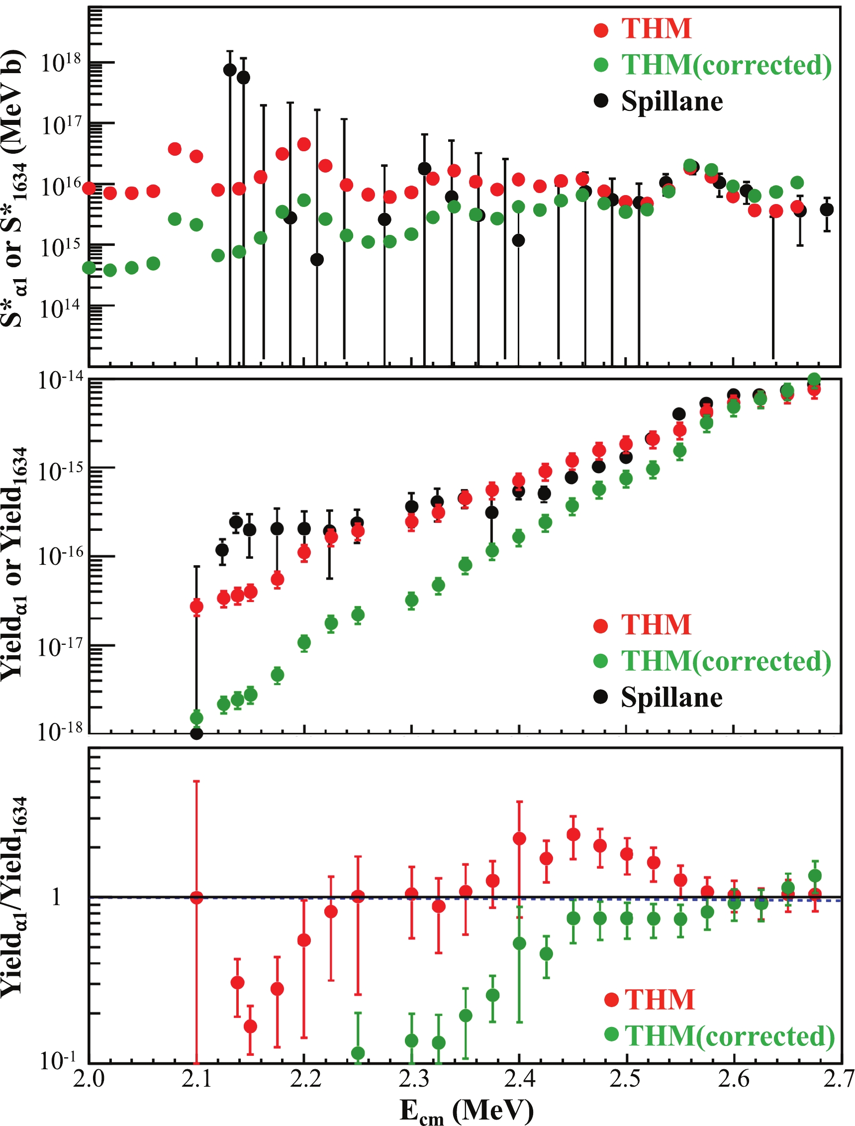Figure12. (color online) (top) S^* factors of $ \alpha_1 $ channel obtained with THM (red), corrected THM (green), and the 1634 keV transition measured by Spillane et al. (black); (middle) Thick target yield measured by Spillane et al. (black) and calculated thick target yields based on THM and corrected THM data sets; (bottom) Thick target ratios of calculated yields based on THM (red) or corrected THM (green) to the one measured by Spillane et al.

The measurements of Becker reported that the ratio of $ \sigma_{\alpha2} $/$ \sigma_{\alpha1} $ ratio is less than 2% at 3.18 MeV and lower energies. Our statistical model predicts this ratio to be below 6% at energies below 3 MeV. Therefore, the $ \alpha_2 $ contribution can be ignored, and the full 1634 keV $ \gamma $ ray yield is considered to be of the $ \alpha_1 $ channel. The THM measurement normalized the $ \alpha_1 $ channel to the total S^* factor of the $ \alpha $ channel, which includes the $ \alpha_0 $ channel. Therefore, we must renormalize the $S^*_{\alpha_1} $ factor obtained with THM to the $S^*_{1634} $ factor directly measured by Spillane et al. using the resonance at $ E_{\rm cm} $ = 2.567 MeV.
A comparison of the directly measured S^* factor to the two versions of S^* factors obtained with the THM is shown in Fig. 12. Although some discrepancies have been observed at energies below 2.7 MeV, the large error bars of the measurement by Spillane prevent us from drawing a clear conclusion. The origin of the large errors comes in part from low statistics and from limitations caused by the background level. Another contribution comes from the differentiation process to obtain the cross section from the measured thick target yield. To avoid this uncertainty, we choose to convert the two versions of the THM S^* factors into the thick target yields using the formula in Ref. [5] and compare them with the measured thick target yield of the 1634 keV transition obtained by Spillane et al. The comparison of the thick target yields is shown in Fig. 12.
The ratios of the THM thick target yields to the directly measured thick target yield are also shown at the bottom of Fig. 12. There are two clear disagreements between the S^* factors obtained with indirect and direct measurements. The first disagreement is around 2.14 MeV, where a strong resonance was claimed to occur. To date, there has been no precise direct measurement able to confirm the existence of this resonance. Moreover, it is clear that the two THM thick target yields are lower than Spillane's thick target yield, and the strong resonance claimed to occur at 2.14 MeV does not appear in the indirect measurement. Another evident disagreement occurs between 2.4 to 2.6 MeV. The THM result is nearly a factor of two higher than the direct measurement with a reduced $ \chi^2 $ of 2.88. The calculated thick target yield using the THM S^* factor corrected with the distorted wave approximation is approximately 20% lower than the direct measurement at energies between 2.45 to 2.6 MeV; however, this yield becomes much lower than the direct measurement at lower energies. Based on this comparison of thick target yields, we may conclude that neither THM result agrees with the direct measurement at energies below 2.7 MeV. More and better direct measurements with higher precision are needed at energies below 2.7 MeV to guide the development of the indirect measurement method.

Astrophysically interesting energies range from a few tens keV up to 3 MeV. Extrapolating the averaged ¹²C+¹²C fusion cross section down to stellar energies is inevitable. The complicated resonance structure in ¹²C+¹²C and the lack of reliable measurements at lower energies prevent us from drawing a clear conclusion [39-41]. The standard reaction rate (CF88 [42]) was established using a constant S^*(E) based on the square well penetration factor. The trend of the predicted S^* factor agrees with theoretical calculations of methods that were proposed later, such as the coupled channel calculation (CC-M3Y+Rep), barrier penetration model based on the S?o Paulo potential (SPP), the Krappe-Nix-Sierk potential (KNS) or equivalent Square Well potential (ESW), density-constrained time dependent Hartree-Fock method (DC-TDHF), and wave-packet dynamics (TDWP).
The hindrance model predicts that the ¹²C+¹²C S-factor reaches its maximum around $ E_{\rm cm} $ = 3.68 MeV [43]. At lower energies, this model predicts a rapid drop in the S-factor, leading to a reduced reaction rate that is several orders of magnitude smaller than the standard rate used for astrophysical modeling (see Fig. 13). A satisfactory description of both the ¹²C+¹²C and ¹²C+¹³C cross sections with one set of assumptions and parameters is mandatory for any global model being tested. The recent precise measurement of the ¹²C+¹³C at deep sub-barrier energies clearly rules out the existence of the astrophysical S-factor maximum, predicted by the phenomenological hindrance model, while confirming the trend of the S^* factor towards lower energies predicted by other models, such as CC-M3Y+Rep, DC-TDHF, KNS, SPP, and ESW [32]. A recent TDHF calculation also claims the absence of hindrance in ¹²C+¹²C [44].
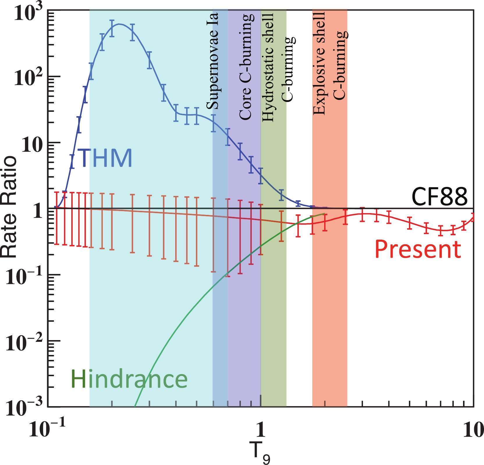Figure13. (color online) Rates relative to CF88 rate [42] obtained in the present study (red) along with rates based on the THM measurement [35] (blue) and hindrance model [43] (Green). Temperatures for the type Ia supernovae (T = 0.15-0.7 GK), core carbon burning (T = 0.6-1.0 GK), hydrostatic shell carbon burning (T = 1.0-1.2 GK), and explosive shell carbon burning (T = 1.8-2.5 GK) are marked by colored bands.

The strong correlation among the carbon isotope systems provides a great opportunity to establish an upper limit for the ¹²C+¹²C S^* factor using models constrained by ¹²C+¹³C or ¹³C+¹³C [5]. Later, this correlation was explained by the ANL group using the large differences of level densities between ¹²C+¹²C and other carbon isotope systems [45]. The upper limit obtained with ¹²C+¹³C has been reported in Ref. [32]. In the present study, we fit the ¹³C+¹³C data using the ESW model. By following the suggestion of Esbensen et al. [43], we scale this original data by a factor of 1.2 in our fitting. The best fit is achieved with the parameters V = –4.01093 MeV, W = 1.02877 MeV, and R = 7.35012 fm. The upper limit of ¹²C+¹²C is obtained by scaling R with (12/13)^(1/3). The two upper limits are shown in Fig. 10 (d). Although both limits provide a good upper bound for the total S^* factor of ¹²C+¹²C, there are minor differences between them. The upper limit obtained with ¹²C+¹³C is higher than the upper limit obtained with ¹³C+¹³C by 30% around $ E_{\rm cm} $ = 4.2 MeV. This difference has been explained by the coupling effect of neutron transfer in the ¹²C+¹³C fusion reaction [43]. At energies below 3 MeV, the effect from the transfer reaction becomes negligible, and the two limitations agree with each other with a difference below 17%, a value similar to the experimental errors of the fusion cross section measurements at sub-barrier energies.
The direct measurement by Spillane et al. [16] reported a strong resonance at 2.14 MeV. Considering the large uncertainty, the direct measurement is higher than the upper limit by only 1.87$ \sigma $. It has been discussed above that the indirect measurement does not support the existence of this resonance. Therefore, one has to wait for a better measurement to tell whether such a resonance exceeding the theoretical upper limit exists.
The lower limits presented in the present study include an empirical lower limit (KNS) and a theoretical calculation (TWDP) [32]. The current TDWP approach does not include the cluster effect and only provides a baseline for the ¹²C+¹²C S^* factor at lower energies. It is interesting to note that the TDWP calculation agrees with the empirical lower limit (KNS) with a deviation below 33% at energies below 3 MeV. Combining the new upper limits with the empirical lower limit and the prediction of TDWP, the ¹²C+¹²C S^* factors are better constrained despite the unknown resonances within the unmeasured energy range.

The reaction rate of ¹²C+¹²C is calculated with the measured S^* factors at E$ _{\rm cm}> $2.7 MeV, where a reasonable agreement among the experimental total S^* factors exists, and using the lower and upper limits for $ E_{\rm cm}< $2.7 MeV. The corrected S^* factor obtained in measurements by Spillane et al. is used in the range of 2.7 to 4.4 MeV. The corrected S^* factor obtained with the measurement by Kettner et al. is used in the range of 4.4 to 6.3 MeV. A ±30% uncertainty is used to account for the deviation among different experimental data sets, as well as the systematic errors of the statistical model in addition to the statistical errors. The theoretical fusion cross section is used for higher energies [46] with an assumed 10% uncertainty to account for the experimental error. For the energies below 2.7 MeV, the upper limit obtained with ¹³C+¹³C and the lower limit from the TDWP prediction were used, as they represent the highest and lowest limits, respectively. The assumption is made that there is no extremely strong resonance structure (such as the significantly enhanced rate values from 0.14 to 0.4 GK reported by Tumino et al. [35]) for low-temperature rates. The average of these two limits is used as the averaged values for the S^* factor. The resulting reaction rates are listed in Table 6. The ratio of the current reaction rate to the standard CF88 [42] rate is shown in Fig. 13 together with the rates obtained with the hindrance model and the THM indirect measurement.

T9	rate/(${\rm cm^3 mol^{-1} s^{-1}}$)	relative uncertainty (1$\sigma$)
0.11	7.61E-50	72%
0.12	1.06E-47	72%
0.13	8.78E-46	73%
0.14	4.70E-44	73%
0.15	1.75E-42	73%
0.16	4.76E-41	74%
0.18	1.65E-38	74%
0.2	2.53E-36	75%
0.25	5.97E-32	77%
0.3	1.27E-28	78%
0.35	5.73E-26	80%
0.4	8.77E-24	81%
0.45	6.13E-22	82%
0.5	2.36E-20	83%
0.6	9.48E-18	86%
0.7	1.12E-15	87%
0.8	5.64E-14	85%
0.9	1.53E-12	79%
1	2.60E-11	70%
1.25	7.17E-09	48%
1.5	5.07E-07	36%
1.75	1.56E-05	31%
2	2.76E-04	28%
2.5	2.56E-02	25%
3	7.18E-01	23%
3.5	8.98E+00	22%
4	6.47E+01	21%
5	1.17E+03	20%
6	8.87E+03	18%
7	3.99E+04	17%
8	1.27E+05	16%
9	3.20E+05	15%
10	6.79E+05	14%

Table6.Recommended reaction rate for ¹²C+¹²C.

Both particle and $ \gamma $-ray spectroscopies have been used to investigate the decay channels of ¹²C+¹²C. By summing the S^* factors of the ground state transitions ($ p_0 $ and $ \alpha_0 $) and the transitions of main characteristic $ \gamma $-rays (440 and 1634 keV) and correcting for the missing channels using a statistical model, an agreement within ±30% deviation has been achieved among allmeasurements at energies $ E_{\rm cm}> $4 MeV. The systematic uncertainty of the statistical model is estimated to be 9% ($ 1\sigma $). At lower energies, although measurements by $ \gamma $-ray spectroscopy [16, 34] agree with each other, some discrepancies remain among particle spectroscopy measurements. These disagreements arise from four possible sources: 1) underestimation of the beam-induced background; 2) incomplete measurement of the decay channels populating the higher excited states or erroneous correction for the missing channels; 3) experimental errors, such as those of target thickness and effective energy determination; and 4) angular distribution of the particles and $ \gamma $ rays. It has been pointed out that the assumption of isotropic angular distribution often used in the charged particle spectroscopy at lower energies may lead to a 20% error [47]. Complete measurements of the angular distributions with good statistics would be useful to reduce this error.
To suppress the background, the particle-$ \gamma $ coincidence measurement was performed using the ATLAS accelerator at Argonne National Laboratory with coincidence between GammaSphere and large area strip silicon detectors [17]. From the particle-$ \gamma $ coincidence spectrum at $ E_{\rm cm} $ = 5.0 MeV from Ref. [48], the characteristic $ \gamma $ rays in the p-channel can be clearly identified. The particle-$ \gamma $ coincidence technique [17] can eliminate the background, and record the $ p_i $-$ \gamma $ and $ \alpha_i $-$ \gamma $ events with a clean background. The random-coincidence events must be well-studied to ensure accuracy. This measurement was further extended down to 2.16 MeV by the STELLA collaboration [18, 49]. However, a more recent measurement of the $ \alpha_1 $ channel [19] is almost a factor of 10 less than the measurements of Beckeret al. [10] and Jiang et al. [17] around $ E_{\rm cm} $ = 2.94 MeV, calling for further measurements at these energies to resolve the discrepancies.
Fruet et al. [18] and Tan et al. [19] both measured $ p_1 $-$ \gamma $(440) and $ \alpha_1 $-$ \gamma $(1634) coincidence events at very low energies and subsequently provided total cross sections for proton and alpha channels by normalizing their $ \sigma_{p_1} $ and $ \sigma_{\alpha_1} $ values using the ratios $ \sigma_{p_1} $/$ \sigma_{p} $ and $ \sigma_{\alpha_1} $/$ \sigma_{\alpha} $ from Becker et al. [10]. In reference [49], these ratios are $ \sigma_{p_1} $/$ \sigma_{p} $ = (15.6 ± 0.7)% and $ \sigma_{\alpha_1} $/$ \sigma_{\alpha} $ = (31.9 ± 1.4)%, which are only mean values, ignoring the large fluctuations (see Fig. 27 of Set. 3 in Ref. [49]). However, according to the present analysis in Fig. 6 and Fig. 7, the standard deviations for the $ \sigma_{p_1} $/$ \sigma_{p} $ and $ \sigma_{\alpha_1} $/$ \sigma_{\alpha} $ ratios of Becker et al. [10] are 42% and 26%, respectively. Therefore, it is important to recognize that large uncertainties exist in the total cross sections of $ \sigma_{p} $ and $ \sigma_{\alpha} $ that are derived only from $ \sigma_{p_1} $ and $ \sigma_{\alpha_1} $ and their corresponding branching ratios $ \sigma_{p_1} $/$ \sigma_{p} $ and $ \sigma_{\alpha_1} $/$ \sigma_{\alpha} $, as recently reported by Fruet et al. [18] and Tan et al. [19].
Our statistical model calculation based on the data obtained with particle spectroscopy shows that the relative systematic uncertainties of the predicted branching ratios decrease as the branching ratios increase. Although the particle-$ \gamma $ coincidence measurements offer a clean background, deriving the total S^* factors for the proton and alpha channels only from the $ p_1 $-$ \gamma $(440) or $ \alpha_1 $-$ \gamma $(1634) events at astrophysical energies would suffer from fluctuations arising from the complicated resonances in the ¹²C+¹²C system, shown in Fig. 6 and Fig. 7. Furthermore, the resonances of $ p_1 $ or $ \alpha_1 $ do not necessarily represent the resonances of p- or $ \alpha $- channels. Therefore, to effectively derive the total fusion cross sections of ¹²C+¹²C, we propose measuring the ground states of the $ \alpha $- and p- channels ($ \alpha_0 $,$ p_0 $) together with the particle channels in coincidence with the 440, 1634, 2391, 2640, and 2982 keV characteristic $ \gamma $ rays to cover the $ p_1 $, $ \alpha_1 $, $ p_2 $, $ p_3 $ and $ p_4 $ channels, which would limit the systematic errors in the branching ratios. Our calculation also shows that a constant branching ratio is the best choice for deriving the S^* factors of ¹²C(¹²C,$ \alpha $)²⁰Ne and ¹²C(¹²C,p)²³Na from the measured partial S^* factors.
The ground state transitions are crucial, as these channels contribute significantly at stellar energies (Fig. 6 and Fig. 7). Novel technologies are required to suppress the backgrounds. As a complement for the particle-$ \gamma $ coincidence technique, a solenoid spectrometer has been applied for investigating the ground state decay channels of ¹²C+¹²C fusion [50]. An efficient thick target method based on particle spectroscopy has indicated great potential by scanning for the existence of potential resonances through a wide energy range with only a single incident energy [51]. Particle identification techniques, such as $ \Delta $E-E and TOF-E, are useful to identify protons and $ \alpha $ particles at energies around 1 MeV and effectively suppress the beam-induced and cosmic backgrounds [13, 49]. The rather large contribution of the $ \alpha $ transfer channel, ¹²C(¹²C,⁸Be)¹⁶O reported at energies below 3 MeV, must be investigated both theoretically and experimentally to clarify its role at stellar energies.
The large uncertainty in the astrophysical reaction rate of ¹²C+¹²C is created mainly by the extremely low-trend predicted by the hindrance model [43], which is independent of the resonance structure, and the recent THM result [35], which predicts a very high reaction rate (see Fig. 13). The resonance structure itself makes it difficult experimentally to discern between the various predictions. Our upper and lower limits are established empirically based on the carefully evaluated data obtained by direct measurements. These limits present a novel approach to extrapolate the ¹²C+¹²C S^* factors down to the important energy region. They significantly reduce the existing uncertainties in the extrapolation. It is important to test these limits with the precise direct measurements to be performed at energies below 2.7 MeV. If there are currently unknown relatively strong resonances, which are fundamentally different from the resonances already confirmed by observing direct measurements at energies above 2.7 MeV, the upper and lower limits presented in the present study must be revised.

In summary, we calculated the branching ratios of numerous states in the $ \alpha $- and p- channels for the ¹²C+¹²C fusion based on the statistical model. The theoretical branching ratios are compared with the experimental branching ratios measured with particle spectroscopy. The theoretical results in the present study reproduce the averaged trend of the branching ratios for p_i and typical characteristic $ \gamma $ rays (E_γ = 440 keV) in ¹²C(¹²C,p)²³Na and α_i and typical characteristic $ \gamma $ rays (E$ _\gamma $ = 1634 keV) in ¹²C(¹²C,$ \alpha $)²⁰Ne. Our calculations show that the relative systematic uncertainties of the predicted branching ratios decrease as the predicted ratios increase. Various data sets obtained with $ \gamma $ or particle spectroscopies are corrected for the missing channels, and reasonable agreements among the S^* factors of the proton, $ \alpha $ particle, and their summation are achieved at energies above 2.7 MeV. Upper and lower limits are recommended for energies below 2.7 MeV. A new ¹²C+¹²C reaction rate is also recommended. Further, the indirect measurement performed with the THM is found to be inconsistent with the direct measurement by comparing the thick target yield of the 1634 keV $ \gamma $-ray transition. Better measurements at energies below 4 MeV are required to resolve discrepancies among existing measurements. Reliable measurements at 2.7 MeV are particularly needed to guide the development of extrapolating models, calibrate the theory for indirect measurements, and verify the proposed upper and lower limits used in the extrapolation.
X.D. Tang acknowledges Dr. Kettner for providing the original data of his work.