Hang Yang
, Qichun Feng
, Yanyv Ren
, Jingbo Zhang ^,
, Lei Huo
,

Corresponding author: Jingbo Zhang, jinux@hit.edu.cn

School of Physics, Harbin Institute of Technology, Harbin 150001, China
Received Date:2019-09-12
Accepted Date:2019-12-13
Available Online:2020-05-01
Abstract:We analyze the transverse momentum dependence of HBT radii in relativistic heavy-ion collisions using several source models. Results indicate that the single-particle space-momentum angle distribution plays an important role in the transverse momentum dependence of HBT radii. In a cylinder source, we use several formulas to describe the transverse momentum dependence of HBT radii and the single-particle space-momentum angle distribution. We also make a numerical connection between them in the transverse plane.

HTML

--> --> -->

A new state of matter has been found in the Relativistic Heavy Ion Collider, called quark-gluon-plasma (QGP) [1-3]. It is strongly interacting partonic matter formed by deconfined quarks and gluons under extreme temperature and energy density. This state is similar to the early time of the universe after the Big Bang [4], and it has aroused great interest in the physics community. A powerful tool in studying the mechanism of particle production in hot QCD matter is the two-pion intensity interferometry. The interferometry analyses were first performed by Hanbury Brown and Twiss to measure the angular diameter of stars in the 1950s, and hence obtained the name, HBT method. G. Goldhaber, S. Goldhaber, W. Lee and A. Pais extended this method in $ \overline{p}+p $ collisions [5]. Since, the two-pion interferometry has been widely used in high-energy heavy-ion collisions, with significant development and improvement. For example, the HBT radii parameters may be used to locate the critical end point (CEP) in the QCD phase diagram [6], and the multi-pion interferometry has been used in high-energy heavy-ion collisions as an extension of two-pion interferometry [7-9].
Many collaborations use the HBT method to analyze different collisions at different energies [10-14]. Most of them show the phenomenon of transverse momentum or transverse mass dependence of HBT radii. The shrinking of HBT radii with increasing transverse momentum is associated with collective flow [15,16]. At the energy range of the Beam Energy Scan Phase II (BES-II) at RHIC, the flow is not as strong compared with the flow at the LHC energy range [17]. Thus, when the particles freeze out, there will be a finite angle between the radius and the momentum vectors. We named this the single-particle space-momentum angle $ \Delta\varphi $. Figure 1 is illustrates a diagram of this angle and its projection angle $ \Delta \theta $ on the transverse plane.
Figure1. Diagram depicting $\Delta\varphi$ and $\Delta \theta$. $\Delta\varphi$ is angle between $\vec r$ and $\vec p$, and $\Delta \theta$ is angle between $\vec r_{\rm T}$ and $\vec p_{\rm T}$ at freeze out time. The origin represents the center of the source.

We use locally thermalized fireballs with the collective flow to produce particles, which are the same as the blast wave model [18]. The blast wave model has already been used in analyses of the HBT correlations [19-21], and it can also be used to describe the transverse momentum dependence on HBT radii [22,23]. The space-momentum correlation has a large influence on the HBT radii. In this study, we use the single-particle space-momentum angle distribution to describe the space-momentum correlation. We focus on the $ \Delta\varphi $ distribution effect on the transverse momentum dependence of HBT radii. Subsequently, we attempt to build a new connection between the $ \Delta \theta $ distribution and the transverse momentum dependence of HBT radii in the transverse plane. Through this connection, we can use the single-particle space-momentum angle distribution to describe the transverse momentum dependence of HBT radii in the transverse plane.
This paper is structured as follows. Sec. 2 briefly introduces the CRAB code and the method used to calculate the HBT radii. In Sec. 3, we calculate the HBT radii for pions in different sources. In Sec. 4, a numerical connection has been built between the $ \Delta \theta $ angle distribution and the transverse momentum dependence of $ R_{\rm o} $, $ R_{\rm s} $. Finally, we summarize our conclusions in Sec. 5.

We use the correlation after burner (CRAB) code to read the phase-space information of generated pions and calculate the two-pion correlation functions [24]. The code is based on the formula

$ C({{q}},{{K}}) = 1+\frac{\int {\rm d}^4x_1 {\rm d}^4x_2 S_1(x_1,{ p}_2) S_2(x_2,{ p}_2) {\left|\psi_{\rm{rel}} \right|}^{2}} {\int {\rm d}^{4}x_{1}{\rm d}^{4}x_{2}S_{1}(x_{1},{ p}_{2})S_{2}(x_{2},{ p}_{2})}, $

(1)

where $ { q} = { p}_1-{ p}_2 $, $ { K} = ({ p}_1+{ p}_2)/2 $, and $ \psi_{\rm{rel}} $ is the two particle wave function. In further discussion, we neglect the Coulomb interaction and strong interactions between pions. The correlation functions can be calculated in different $ p_{\rm T} $ bins by changing the kinematic cuts in the fitter of the CRAB code. We use the single-pion information extracted from the calculation to analyze the space-momentum angle $ \Delta\varphi $ distribution.
We usually use the ‘out-side-long’(o-s-l) coordinate system in the HBT research, shown in Fig. 2. The longitudinal direction is along the beam direction, and the transverse plane is perpendicular to the longitudinal direction. In the transverse plane, the momentum direction of pair particles is the outward direction. The direction perpendicular to the outward direction is referred to as the sideward direction.
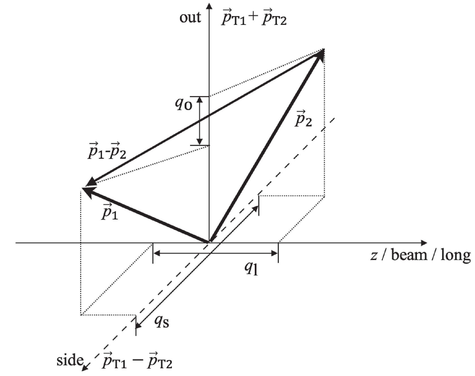Figure2. The diagram of ‘out-side-long’(o-s-l) coordinate system.

In the calculation of the HBT correlation function, the rapidity range is consistently set to $ -0.5<\eta<0.5 $. An example of correlation functions of a Gaussian source is shown in Fig. 3. They are in $ q_{\rm o} $ and $ q_{\rm s} $ directions, with $ -3<q_{\rm l}<3 $ MeV/c.
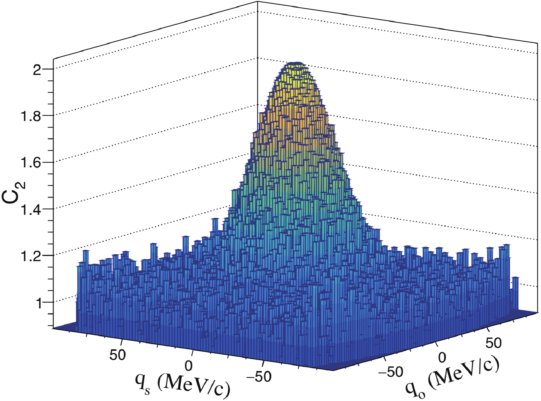Figure3. (color online) HBT correlation function in $q_{\rm o}$ and $q_{\rm s}$ directions for a Gaussian source.

The HBT correlation function of the Gaussian form can be written as [25]

$ C({{q}},{{K}}) = 1+\lambda {\exp} {[-q_{\rm o}^2 R_{\rm o}^2({ K})-q_{\rm s}^2 R_{\rm s}^2({ K})- q_{\rm l}^2 R_{\rm l}^2({ K})]}, $

(2)

where $ \lambda $ is the coherence parameter. $ R_{\rm i}^2 $ can be expressed as [26,27]

$R_{\rm{s}}^2 = \langle r_{\rm{s}}^2\rangle ,$

(3)

$R_{\rm{o}}^2 = \langle {({r_{\rm{o}}} - {\beta _{\rm{o}}}t)^2}\rangle - {\langle {r_{\rm{o}}} - {\beta _{\rm{o}}}t\rangle ^2},$

(4)

$R_{\rm{l}}^2 = \langle {({r_{\rm{l}}} - {\beta _{\rm{l}}}t)^2}\rangle - {\langle {r_{\rm{l}}} - {\beta _{\rm{l}}}t\rangle ^2},$

(5)

where the average notation is defined as

$\langle \xi \rangle = \frac{{\int {{{\rm d}^4}} x\xi S(x,p)}}{{\int {{{\rm d}^4}} xS(x,p)}}.$

(6)

We can calculate the HBT radii using Eq. (2) to fit the HBT correlation function, which is generated from the CRAB code.

The single-particle momentum space angle distribution, i.e., $ \Delta\varphi $ angle distribution, can directly cause transverse momentum $ p_{\rm T } $ dependence.
First, the influence of the source lifetime must be excluded. Using a Gaussian source to generate pion data, the emission function can be written as

$ S(x,{ p}) = A{ p}^{2}{\rm{exp}}\left(-\frac{\sqrt{{ p}^2+m^2}}{T}\right) {\rm{exp}}\left(-\frac{{ r}^2}{2R^2}-\frac{t^2}{2(\Delta t)^2}\right), $

(7)

where we set source size $ R = 6.0 $ fm, temperature $ T = 100 $ MeV, and mass of pions $ m = 139.58 $ $ \rm MeV/c^2 $. Then, we use the CRAB code to calculate the HBT correlation functions of pions. Afterwards, we use Eq. (2) to fit the correlation functions in different $ p_{\rm T} $ bins, and there are nine bins in 125 MeV/c $ <p_{\rm T}< $ 625 MeV/c. The transverse momentum dependence of HBT radii are shown in Fig. 4.
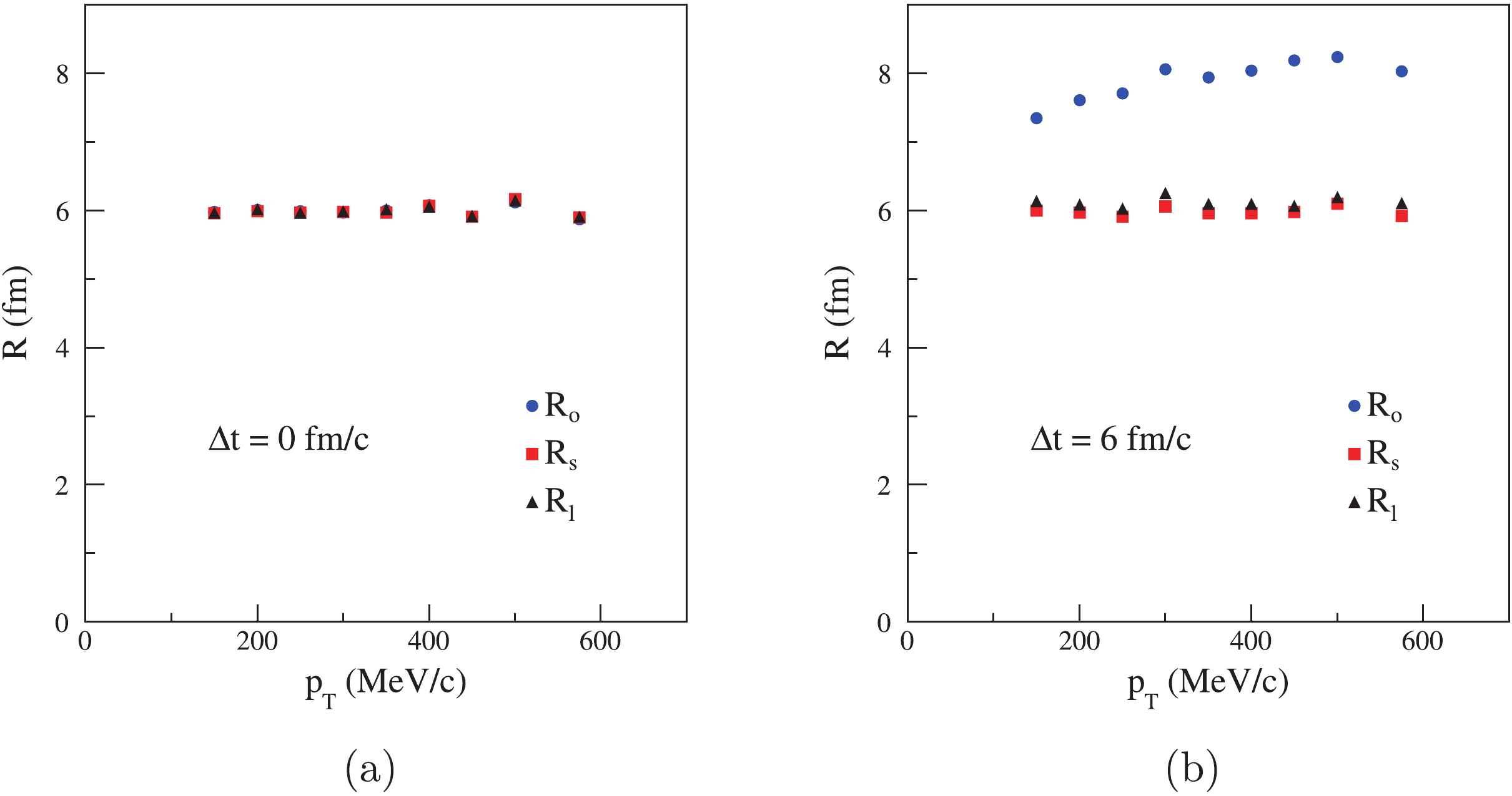Figure4. (color online) Transverse momentum dependence of HBT radii for a Gaussian source.

In Fig. 4(a), when the lifetime of source is $ \Delta t = 0 $ fm/c, all pions freeze out at the same time. The HBT radii coincide with each other, and they are almost equal to the source radii. There is no transverse momentum dependence of HBT radii. With $ \Delta t = 6 $ fm/c, as shown in Fig. 4(b), the value of $ R_{\rm{o}} $ increases gradually with the $ p_{\rm T} $. There is little changes of $ R_{\rm{l}} $ and $ R_{\rm{s}} $. Then, we calculate the HBT radii by changing the value of $ \Delta t $ in Fig. 5.
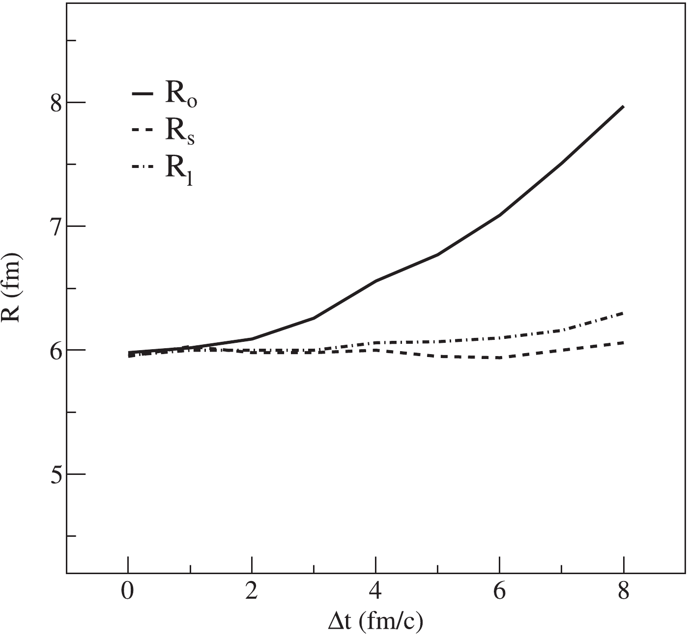Figure5. HBT radii changes with $\Delta t$ for a Gaussian source.

In Fig. 5, the Gaussian source radius remains at 6 fm, and the transverse momentum range is 125–625 MeV/c. We can see the increase of $ R_{\rm o} $ at higher lifetime $ \Delta t $ of the source. Because the rapidity cut is $ -0.5<\eta<0.5 $, $ R_{\rm l} $ only changes slightly. There is barely any change in $ R_{\rm s} $. As the emission function of the Gaussian source is known, using Eqs. (3)–(7), the HBT radius can be expressed as

$R_{\rm{s}}^2 = \langle r_{\rm{s}}^2\rangle ,$

(8)

$R_{\rm{o}}^2 = \langle r_{\rm{o}}^2\rangle + {\langle {\beta _{\rm{o}}}\rangle ^2}\langle {(\Delta t)^2}\rangle ,$

(9)

$R_{\rm{l}}^2 = \langle r_{\rm{l}}^2\rangle + {\langle {\beta _{\rm{l}}}\rangle ^2}\langle {(\Delta t)^2}\rangle ,$

(10)

where r and $ \beta $ are space coordinate and velocity of a single particle, respectively. Therefore, we can reduce the influence of the lifetime of the source by minimizing $ \Delta t $.
To discuss the influence of the single-particle angle distribution on the transverse momentum dependence of HBT radii, we introduce another source, i.e., the space-momentum angle correlation source. The emission function can be written as

$ S(x,{ p}) = A{ p}^{2}{\rm{exp}}\left(-\frac{\sqrt{{ p}^2+m^2}}{T}\right) {\rm{exp}}\left(-\frac{{ r}^2}{2R^2}-\frac{t^2}{2(\Delta t)^2}\right) {\rm w}\left(\Delta \varphi\right), $

(11)

where $ \Delta \varphi $ is the single-pion space-momentum angle at freeze-out time. By changing the formula of $ {\rm{w}}\left(\Delta \varphi\right) $, we can change the angle $ \Delta \varphi $ distribution. If $ {\rm{w}}\left(\Delta \varphi\right) = 1 $, the $ \Delta \varphi $ value is entirely random between $ 0-\pi $, and the source becomes a Gaussian source. Here, the function $ \rm w $ in Eq. (11) can be written as

${\rm{w}}\left( {\Delta \varphi } \right) = \left\{ {\begin{array}{*{20}{l}}0&{\alpha {\rm{ < }}\Delta \varphi \leqslant \pi }\\1&{0 \leqslant \Delta \varphi \leqslant \alpha }\end{array}} \right.,$

(12)

where $ \alpha $ is a given value. This function indicates that only the pions whose angle $ \Delta \varphi $ is smaller than the $ \alpha $ value can exist. The radius of the source is $ R = 6 $ fm, and the lifetime is $ \Delta t = 0 $ fm/c.
In Fig. 6(a), $ \alpha = \frac{\pi}{2} $. $ R_{\rm{o}} $ values are lower than $ R_{\rm{s}} $ and $ R_{\rm{l}} $, and the HBT radii are mostly flat as a function of $ p_{\rm T} $. There is barely any appearance of $ p_{\rm T} $ dependence. In Fig. 6(b), $ \alpha = \frac{\pi}{3} $. Compared with Fig. 6(a), the values of $ R_{\rm{s}} $ and $ R_{\rm{l}} $ become smaller. The values of $ R_{\rm{o}} $ change slightly. The present work shows that the $ \Delta\varphi $ distribution can affect the values of HBT radii. Furthermore, we nevertheless use the space-momentum angle correlation source to generate the data, the emission function and the w function are still based on Eqs. (11) and (12), while $ \alpha $ varies between 0 and $ \pi $. The HBT radii as the function of $ \cos\alpha $ value are shown in Fig. 7.
Figure6. (color online) HBT radii for a space-momentum angle correlation source.

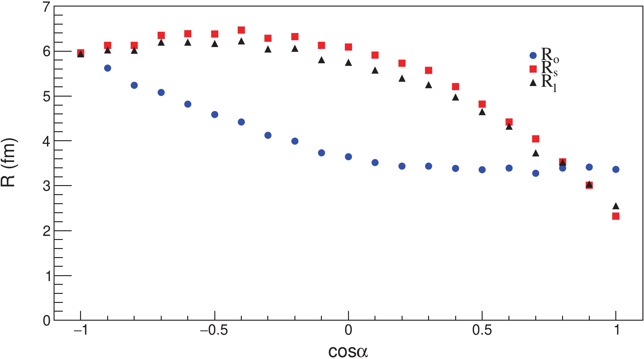Figure7. (color online) $\cos \alpha$ dependence of HBT radii for a space-momentum angle correlation source.

In Fig. 7, the transverse momentum range is 125–625 MeV/c. When $ -1<\cos\alpha<0 $, the $ R_{\rm{o}} $ values decrease with increasing $ \cos\alpha $, while $ R_{\rm{s}} $ and $ R_{\rm{l}} $ only exhibit small changes. When $ 0<\cos\alpha<1 $, there are almost no changes in $ R_{\rm{o}} $, while $ R_{\rm{s}} $ and $ R_{\rm{l}} $ decrease with increasing $ \cos\alpha $. The various space-momentum angle $ \Delta\varphi $ distributions correspond to different HBT radii. Therefore, if we can control the $ \Delta\varphi $ angle distribution for a given $ p_{\rm T} $, we can reproduce the $ p_{\rm T} $ dependence phenomenon.
We use a homogeneous expansion source to calculate the HBT radii in different $ p_{\rm T} $ regions, and subsequently we use space-momentum angle correlation source to reproduce this phenomenon. The homogeneous expansion source is based on the Gaussian source. Every pion has been given an expansion velocity $ { \beta }$ along the $ { r} $ direction. The momentum is generated using the Lorentz transformation. The emission function can be written as

$ S = A{ p}^{2}{\rm{exp}}\left(-\frac{\gamma E-\gamma{ {\beta p}}}{T}\right) {\rm{exp}}\left(-\frac{{ r}^2}{2R^2}-\frac{t^2}{2(\Delta t)^2}\right), $

(13)

where $ \gamma = 1/\sqrt{1-\beta^2} $ is the Lorentz factor, still with $ R = 6 $ fm and the $ \Delta t = 0 $ fm/c. After using this emission function to generate data, we use the CRAB code to calculate correlations and Eq. (2) to calculate the HBT radii in different $ p_{\rm T} $ regions. Meanwhile, we can also obtain the phase-space information of pions in different $ p_{\rm T} $ regions. The equation to fit the normalized space-momentum angle distribution can be written as

$ f(\Delta\varphi) = c_1{\rm{exp}}(c_2\cos(\Delta\varphi)), $

(14)

where $ c_1 $ and $ c_2 $ are fit parameters. The fit lines are shown in Fig. 8.
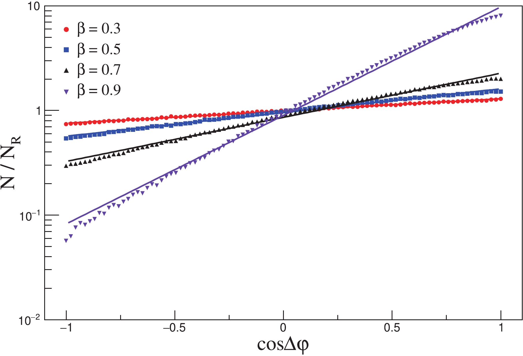Figure8. (color online) Fit normalized $\cos(\Delta\varphi)$ for different homogeneous expansion sources. The transverse momentum range is 125–175 MeV/c. The dots are normalized numbers of pions, and the lines depict fits.

There are nine bins of $ p_{\rm T} $, and we have nine groups of two parameters $ c_1 $ and $ c_2 $. Subsequently, we use the space-momentum angle correlation source to simulate the HBT radii. In the emission function of Eq.(11), $ {\rm{w}}(\Delta\varphi) = f(\Delta\varphi) $. We insert the values of $ c_1 $ and $ c_2 $ into this equation, and each $ p_{\rm T} $ region corresponds to one emission function, such that there are nine emission functions. We use each emission function to generate the data and calculate the HBT radii in the corresponding $ p_{\rm T} $ region, and both particles are taken from the same $ p_{\rm T} $ region. After the calculation, the simulation results and HBT radii calculated by homogeneous expansion sources are shown in Fig. 9.
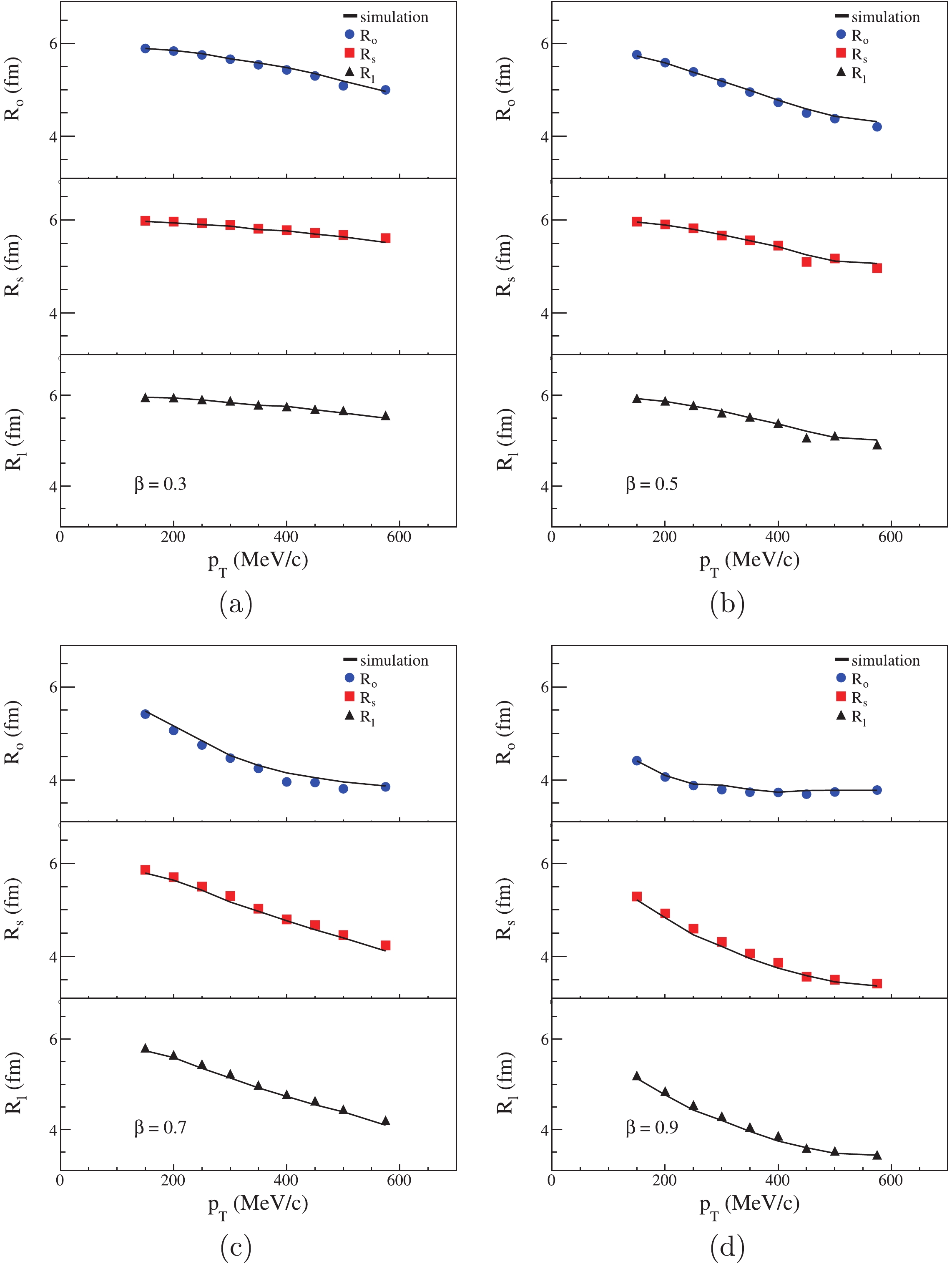Figure9. (color online) Simulation for a homogeneous expansion source. Black simulation lines are calculated in space-momentum angle correlation source.

For all four situations in Fig. 9, the simulated HBT radii are almost equal to the HBT radii calculated in the homogeneous expansion sources. This indicates that the source expansion can cause the space-momentum angle $ \Delta\varphi $ distribution narrowing with transverse momentum. This meets our expectation that the different space-momentum angle $ \Delta\varphi $ distributions lead to different values of HBT radii, which subsequently causes the transverse momentum dependence of HBT radii.

We use the cylinder expansion source [27] to obtain the connection between the HBT radii and $ \Delta \theta $(angle between $ \vec p_{\rm T} $ and $ \vec r_{\rm T} $) distribution. This can be written as

$\begin{split}S\left( {x,p} \right) =& A{M_{\rm{T}}}\cosh \left( {\eta - Y} \right){\rm{exp}}\left( { - \frac{{pu\left( x \right)}}{T}} \right)\\&\times\exp \left( { - \frac{{{{\left( {\tau - {\tau _0}} \right)}^2}}}{{2{{\left( {\delta \tau } \right)}^2}}} - \frac{{{\rho ^2}}}{{2R_{\rm{g}}^2}} - \frac{{{\eta ^2}}}{{2{{\left( {\delta \eta } \right)}^2}}}} \right),\end{split}$

(15)

where $ u(x) $ is the four-velocity, which can be decomposed as

$ u(x) = \left( \cosh\eta\cosh\eta_{\rm T},\sinh\eta_{\rm T}\vec{e}_{\rm T},\sinh\eta\cosh\eta_{\rm T} \right), $

(16)

and $ \eta = \frac{1}{2}\ln[(p+z)/(p-z)] $ is the longitudinal flow rapidities. The transverse flow rapidity is defined as

${\eta _{\rm{T}}} = \left\{ {\begin{array}{*{20}{l}}{{\eta _{{\rm{Tmax}}}}\frac{\rho }{{{R_{\rm{g}}}}}}&{\rho < {R_{\rm{g}}}}\\{{\eta _{{\rm{Tmax}}}}}&{\rho \geqslant {R_{\rm{g}}}}\end{array}} \right..$

(17)

The rapidity of the pion is $ Y = \frac{1}{2}\ln[(E+p_{\rm l})/(E-p_{\rm l})] $, the proper time is $ \tau = \sqrt{t^2-z^2} $, and the pion radial position in the transverse plane is $ \rho = \sqrt{x^2+y^2} $. We set $ T = 100 $ MeV, $ \delta\tau = 0 $ fm/c, $ \tau_0 $ = 10 fm/c, $ R_{\rm {g}} $ = 6.0 fm, and $ \delta\eta $ = 3.0, and the variable is $ \eta_{\rm Tmax} $.
Since the CRAB filter is set $ -0.5<\eta<0.5 $ and $ \delta\tau = 0 $ fm/c, all pions almost freeze out at the same time ($ \Delta t<1.3 $fm/c). The effect of the source lifetime is negligible. $ \beta_{\rm Tmax} $ are set as 0.1, 0.2, 0.3, 0.4, 0.5, 0.6, then the $ \eta_{\rm Tmax} $ values are calculated by $ \eta_{\rm Tmax} = \frac{1}{2}{\rm ln}\left( \frac{1+\beta_{\rm Tmax}}{1-\beta_{\rm Tmax}} \right) $.
We generate pions that have random $ { p}_{\rm T} $ and random $ { r}_{\rm T} $, and use them to calculate the random $ \cos(\Delta\theta) $ distribution. Then, we use the distribution of $ \cos(\Delta\theta) $, which is calculated from cylinder expansion source and divided by the random $ \cos(\Delta\theta) $ distribution, to obtainthe normalized $ \cos(\Delta\theta) $ distribution. We fit the normalized $ \cos(\Delta\theta) $ distribution with Eq. (14). The fit lines are shown in Fig. 10, and the fit results are listed in Table 1.

$ \eta_{\rm Tmax} $	par	$ p_{\rm T}: $150–250 MeV	250–350 MeV	350–450 MeV	450–600 MeV
0.1003	$ c_1 $	$ 0.9994\pm0.0002 $	$ 0.9990\pm0.0003 $	$ 0.9981\pm0.0003 $	$ 0.9976\pm0.0003 $
	$ c_2 $	$ 0.0339\pm0.0003 $	$ 0.0496\pm0.0004 $	$ 0.0614\pm0.0004 $	$ 0.0852\pm0.0005 $
0.2027	$ c_1 $	$ 0.9985\pm0.0002 $	$ 0.9974\pm0.0003 $	$ 0.9954\pm0.0003 $	$ 0.9924\pm0.0003 $
	$ c_2 $	$ 0.0663\pm0.0003 $	$ 0.0990\pm0.0004 $	$ 0.1299\pm0.0004 $	$ 0.1621\pm0.0005 $
0.3095	$ c_1 $	$ 0.9969\pm0.0002 $	$ 0.9937\pm0.0003 $	$ 0.9905\pm0.0003 $	$ 0.9851\pm0.0003 $
	$ c_2 $	$ 0.1043\pm0.0003 $	$ 0.1485\pm0.0004 $	$ 0.1903\pm0.0004 $	$ 0.2316\pm0.0005 $
0.4236	$ c_1 $	$ 0.9940\pm0.0002 $	$ 0.9887\pm0.0003 $	$ 0.9836\pm0.0003 $	$ 0.9775\pm0.0003 $
	$ c_2 $	$ 0.1443\pm0.0004 $	$ 0.1990\pm0.0004 $	$ 0.2446\pm0.0004 $	$ 0.2842\pm0.0005 $
0.5493	$ c_1 $	$ 0.9890\pm0.0002 $	$ 0.9829\pm0.0003 $	$ 0.9766\pm0.0003 $	$ 0.9718\pm0.0003 $
	$ c_2 $	$ 0.1914\pm0.0004 $	$ 0.2467\pm0.0004 $	$ 0.2893\pm0.0008 $	$ 0.3186\pm0.0005 $
0.6931	$ c_1 $	$ 0.9817\pm0.0003 $	$ 0.9735\pm0.0003 $	$ 0.9683\pm0.0003 $	$ 0.9631\pm0.0004 $
	$ c_2 $	$ 0.2450\pm0.0004 $	$ 0.2945\pm0.0004 $	$ 0.3270\pm0.0005 $	$ 0.3480\pm0.0006 $

Table1.Fit results of normalized $\cos(\Delta\theta)$ distribution.

Figure10. (color online) Fit normalized $\cos(\Delta\theta)$ for different $\eta_{\rm Tmax}$. Dots are normalized numbers of pions, and lines depict fits.

The fits indicate that, with increase of $ p_{\rm T} $ and $ \eta_{\rm Tmax} $, $ c_1 $ becomes smaller and $ c_2 $ becomes larger. We find that $ c_1 $ and $ c_2 $ can be fitted by

${c_1} = {k_1}p_{\rm{T}}^{{j_1}},$

(18)

${c_2} = {k_2}p_{\rm{T}}^{{j_2}},$

(19)

where $ k_1 $, $ k_2 $, and $ j_1 $, $ j_2 $ are fit parameters. The fit lines are shown in Fig. 11.
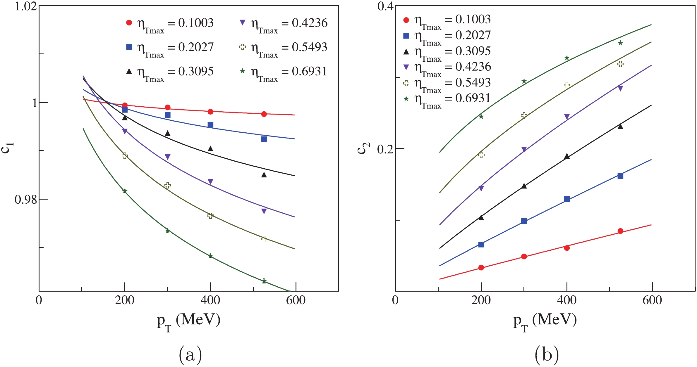Figure11. (color online) Fit $ c_1 $ and $ c_2 $ for different $ \eta_{\rm Tmax} $. Lines depict fits.

We can also fit the HBT radii in different $ p_{\rm T} $ regions by

$R = ap_{\rm{T}}^b,$

(20)

where a and b are fit parameters. The fit lines are shown in Fig. 12.
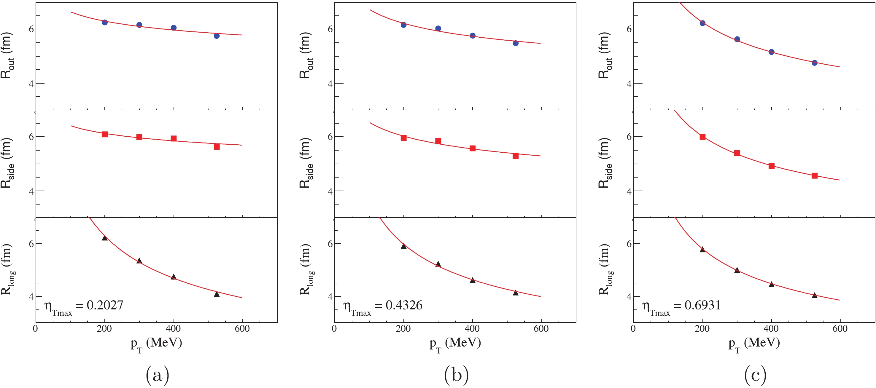Figure12. (color online) Fit HBT radii for different $\eta_{\rm Tmax}$. Red lines depict fits.

In the Fig. 12, there are three cases of $ \beta_{\rm Tmax} = $ 0.2, 0.4, 0.6 for $ \eta_{\rm Tmax} = 0.2027, 0.4236, 0.6931 $. With the increase in $ \eta_{\rm Tmax} $, the transverse flow becomes stronger, and the values of parameter b for $ R_{\rm out} $ and $ R_{\rm side} $ become larger. This indicates that the parameter b describes the strength of $ p_{\rm T} $ dependence, i.e., a larger $ |b| $, indicates a more prominent $ p_{\rm T} $ dependence. Thus, we only focus on the dependence of the $ \Delta \theta $ distribution on the parameter b.
We plot parameters b as the function of k and j in Fig. 13. Because of the longitudinal limit, there is barely any changes in $ b_{\rm long} $. The parameters in out and side directions are basically the same, because the source lifetime is sufficiently small. This means that there is connection between the HBT radii and the $ \Delta \theta $ distribution. The red lines depict fits, and the fit functions are
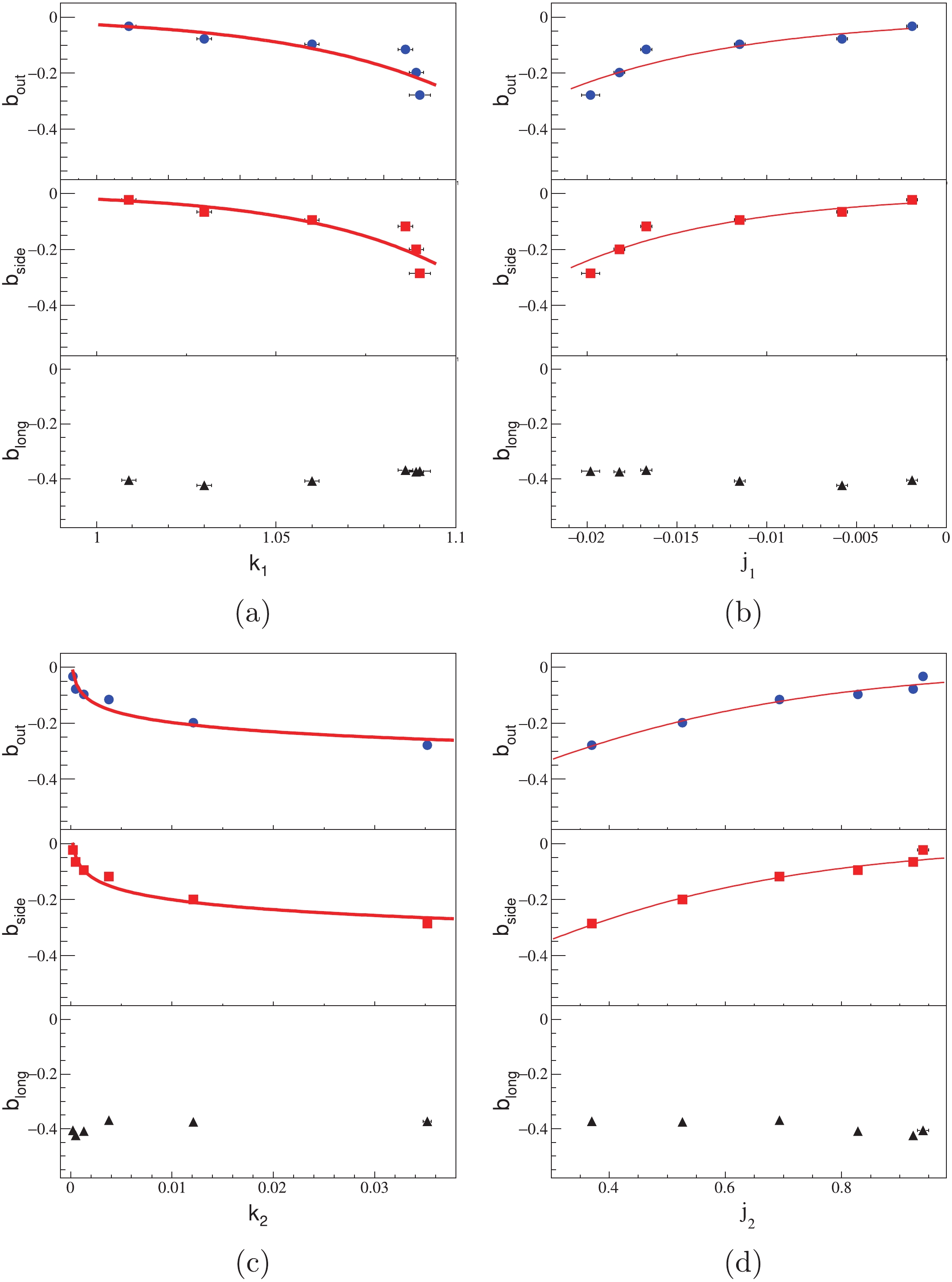Figure13. (color online) Fit parameters in cylinder expansion source. b from HBT radii fit function $R = a p_{\rm T}^{b}$; $j_1$, $j_2$ and $k_1$, $k_2$ from fit functions ${c_1}={k_1}p_{\rm T}^{j_1}$ and ${c_2}={k_2}p_{\rm T}^{j_2}$, respectively; $c_1$ and $c_2$ from normalized space-momentum angle distribution function $f(\Delta\theta)=c_1{\rm{exp}}(c_2\cos(\Delta\theta))$. Red lines depict fits.

$b({k_1}) = {\mu _{11}}{k_1}^{{\mu _{12}}},$

(21)

$b({j_1}) = {\nu _{11}}{{\rm e}^{ - {\nu _{12}}{j_1}}},$

(22)

$b({k_2}) = {\mu _{21}}\ln {k_2} + {\mu _{22}},$

(23)

$b({j_2}) = {\nu _{21}}\left( {\frac{1}{{1 + {{\rm e}^{{\nu _{{\rm{22}}}}{{\rm{j}}_{\rm{2}}}}}}} - 1} \right).$

(24)

The fitted parameter values are shown in Table 2.

Parameters		$ b_{\rm {o}} $	$ b_{\rm {s}} $
$ c_1 $	$ \mu_{11} $	$ -0.026\pm0.001 $	$ -0.021\pm0.001 $
	$ \mu_{12} $	$ -24.3\pm0.5 $	$ -28\pm1 $
	$ \nu_{11} $	$ -0.034\pm0.002 $	$ -0.028\pm0.002 $
	$ \nu_{12} $	$ 97\pm3 $	$ 107\pm4 $
$ c_2 $	$ \mu_{21} $	$ -0.0478\pm0.0006 $	$ -0.0514\pm0.0006 $
	$ \mu_{22} $	$ -0.418\pm0.004 $	$ -0.437\pm0.004 $
	$ \nu_{21} $	$ 1.17\pm0.02 $	$ 1.25\pm0.02 $
	$ \nu_{22} $	$ -3.09\pm0.03 $	$ -3.21\pm0.04 $

Table2.Fit results of $ b(k) $ and $ b(j) .$

A connection has been made between the $ p_{\rm T} $ dependence of HBT radii and the $ \cos(\Delta\theta) $ distribution by Eqs. (21)–(24) and Table 2, in a cylinder source. If all pions freeze out almost at the same time, when we obtain a series of data of $ R_{\rm out} $ or $ R_{\rm side} $ in different $ p_{\rm T} $ regions, we can describe the space-momentum angle distribution as a function of $ p_{\rm T} $ in the transverse plane. If the space-momentum angle distribution is theoretically given as a function of $ p_{\rm T} $, and the $ R_{\rm out} $ or $ R_{\rm side} $ is determined for a given $ p_{\rm T} $ region, we can calculate $ R_{\rm out} $ or $ R_{\rm side} $ in other $ p_{\rm T} $ regions. Because we limit the lifetime of the source, the eight parameters of $ b_{\rm o} $ are similar to the parameters of $ b_{\rm s} $. If the source lifetime increases, $ R_{\rm o} $ will likewise increase, and the parameters of $ b_{\rm o} $ will no longer be valid. Upon changing the model, the parameter values will change as well.

Using several source models, we analyze the effect of the source lifetime and single-particle space-momentum angle distribution on HBT radii. In the mid-rapidity region, $ R_{\rm o} $ is sensitive to the source lifetime. $ R_{\rm o} $ increases rapidly with $ \Delta t $. Furthermore, the HBT radii are also sensitive to the single-particle space-momentum angle distribution. With a decreasing single-particle space-momentum angle, the HBT radii decrease as well. The collective expansion of the source leads to the changes of the single-particle space-momentum angle distribution with different $ p_{\rm T} $, then causes changes of HBT radii, at last, creates the transverse momentum dependence of HBT radii. In transverse plane of a cylinder expansion source, a numerical connection between the transverse momentum dependence of HBT radii and the the single-particle space-momentum angle distribution has been created. The parameters will change according to different sources. If the parameters are settled, we can describe the transverse momentum dependence of HBT radii by the single-particle space-momentum angle distribution.
We appreciate the help of Miaomiao An for discussions on the details of this work. We thank Xiaoze Tan and Weicheng Huang for valuable advice on this manuscript.