HTML
--> --> -->The austral summer (December?January?February, DJF) SAM exhibits a significant positive linear trend during the past half century, which is mainly attributed to Antarctic stratospheric ozone depletion (e.g., Thompson et al., 2011). In contrast, the austral winter (June?July?August, JJA) SAM experienced weaker long-term changes. Models archived in phase 5 of the Coupled Model Intercomparison Project (CMIP5) show noticeable intermodel spread in simulating the long-term changes in both the JJA and DJF SAM (e.g., Swart et al., 2015). The intermodel spread in the JJA SAM is comparable with that in DJF. The JJA SAM plays an important role in influencing Southern Hemisphere extratropical winter climate, including extratropical precipitation (Kidston et al., 2009; Lim et al., 2016), ocean surface waves (Marshall et al., 2018), New Zealand river flow (Li and McGregor, 2017), and Antarctic temperatures (Turner et al., 2005; Fogt et al., 2012). Investigating intermodel spread in simulating temporal variability in the JJA SAM ensures a promising simulation and projection of southern extratropical winter climate.
Studies related to the intermodel difference in the SAM trend involve the intermodel spread in the magnitude of the projected poleward shift of the Southern Hemisphere westerly jet, which has been demonstrated to be related to the simulation of the 20th century climatology (Kidston and Gerber, 2010). Models with the climatological jet position closer to the equator in the 20th century simulation tend to shift the jet further poleward under global warming. However, the variability in the position of the westerly jet, albeit related to, is not equal to the SAM variability (Swart et al., 2015). Examining factors responsible for the intermodel diversity in the SAM’s long-term changes may provide information for improving simulation of the SAM.
Extratropical SST anomalies modulate the overlaying atmospheric baroclinicity (Lau and Nath, 1990; Kushnir et al., 2002), regulate the nonlinear eddy?zonal mean flow interaction (Li et al., 2006; Sen Gupta and England, 2007; Liu et al., 2015; Zheng et al., 2015), and thus influence the extratropical atmospheric circulation (Kang et al., 2008, 2009; Nakamura et al., 2008; Wu et al., 2009; Sampe et al., 2010; Wu and Zhang, 2011; Yang and Wang, 2011; Hu et al., 2016; Xiao et al., 2016). SST anomalies in the Southern Hemisphere middle and high latitudes tend to exhibit an out-of-phase relationship, which is referred to as the Southern Ocean Dipole (SOD) (Zheng et al., 2018). The positive phase of the SOD corresponds to warmer and cooler SST anomalies at around 40°S and 60°S, respectively, and vice versa. Evidence from atmospheric general circulation model (AGCM) simulations shows that the SOD is positively correlated with the SAM during austral winter, suggesting a potential influence of the SOD on the SAM. However, models differ in describing the response of the SAM to the SOD (Zheng et al., 2018). Whether the intermodel uncertainty in depicting the response of the SAM to the SOD contributes to the intermodel difference in the simulated linear trend in the SAM is explored in this study.
The paper is structured as follows: Section 2 introduces the data and methods. The intermodel diversity in the simulated linear trend in the JJA SAM is shown in section 3. Section 4 explores the role of the SOD in the intermodel diversity. Discussion and conclusions are given in section 5.
2.1. Data
The configuration of AGCM runs provides a useful approach to evaluate responses of atmospheric circulation to SST anomalies. AMIP simulations from 28 AGCMs archived in CMIP5 are used in this study. The AMIP runs were constrained using historical SST, and external forcing such as carbon dioxide and ozone concentrations are as in the historical experiment (Taylor et al., 2012). The list of the 28 models is shown in Table 1, and each model is given a short name. Model outputs are interpolated to the same horizontal resolution (1.0° × 1.0°) before statistical analysis. The analysis period of the AMIP simulations covers 1979?2008, and the season of interest is austral winter (June?July?August, JJA).| Model name | Horizontal resolution (Lat × Lon) | Vertical resolution | Short name | |
| Number of levels | Top level (hPa) | |||
| ACCESS1-0 | 145 × 192 | 17 | 10 | A |
| ACCESS1-3 | 145 × 192 | 17 | 10 | B |
| BCC-CSM1.1 | 64 × 128 | 17 | 10 | C |
| BCC-CSM1.1(m) | 160 × 320 | 17 | 10 | D |
| BNU-ESM | 64 × 128 | 17 | 10 | E |
| CanAM4 | 64 × 128 | 22 | 1 | F |
| CCSM4 | 192 × 288 | 17 | 10 | G |
| CESM1-CAM5 | 192 × 288 | 17 | 10 | H |
| CMCC-CM | 240 × 480 | 17 | 10 | I |
| CNRM-CM5 | 128 × 256 | 17 | 10 | J |
| CSIRO-Mk3-6-0 | 96 × 192 | 18 | 5 | K |
| EC-EARTH | 160 × 320 | 16 | 20 | L |
| FGOALS-G2.0 | 60 × 128 | 17 | 10 | M |
| FGOALS-s2 | 108 × 128 | 17 | 10 | N |
| GFDL-CM3 | 90 × 144 | 23 | 1 | O |
| GFDL-HIRAM-C180 | 360 × 576 | 17 | 10 | P |
| GFDL-HIRAM-C360 | 720 × 1152 | 17 | 10 | Q |
| GISS-E2-R | 90 × 144 | 17 | 10 | R |
| HadGEM2-A | 145 × 192 | 17 | 10 | S |
| INMCM4 | 120 × 180 | 17 | 10 | T |
| IPSL-CM5A-LR | 96 × 96 | 17 | 10 | U |
| IPSL-CM5A-MR | 143 × 144 | 17 | 10 | V |
| IPSL-CM5B-LR | 96 × 96 | 17 | 10 | W |
| MIROC5 | 128 × 256 | 17 | 10 | X |
| MPI-ESM-LR | 96 × 192 | 25 | 0.1 | Y |
| MPI-ESM-MR | 96 × 192 | 25 | 0.1 | Z |
| MRI-CGCM3 | 160 × 320 | 23 | 0.1 | a |
| NorESM1-M | 96 × 144 | 17 | 10 | b |
Table1. List of CMIP5 models used in this study and their horizontal and vertical resolutions. The abbreviations “nLat” and “nLon” mean the number of grids in the latitudinal and longitudinal direction, respectively. The short names for each model are listed in the last column.
To detect the spatial pattern of the observed SAM, atmospheric reanalysis data from ERA-Interim are employed. To explore the temporal variability of the observed SAM, the station-based index of the SAM proposed by Marshall (2003) is used, which is characterized by reliability in describing the temporal variability of the SAM, especially before the satellite era.
2
2.2. Statistical methods
Empirical orthogonal function (EOF) analysis is used in this study. The leading EOF pattern and principle component are referred to as EOF1 and PC1. The statistical significance for correlation/regression analysis is assessed by the two-tailed Student’s t-test. Partial correlation is employed to estimate the linkage between two variables after linearly removing effects of the third variable. The intermodel standard deviation quantifies the intermodel spread.According to the method proposed by Nan and Li (2003), the model-simulated SAM index (SAMI) is calculated as the difference in the normalized zonal-mean SLP between 40°S and 70°S. Two other definitions quantifying the temporal variability of the simulated SAM are also used for cross-validation. One is the PC1 from EOF analysis of the SLP south of 20°S (PC1_SLP; Thompson and Wallace, 2000); the other is the PC1 from EOF analysis of the zonal-mean zonal wind south of 10°S (PC1_zmU; Lorenz and Hartmann, 2001). The Ni?o3.4 index is used to represent the ENSO variability. Spline interpolation is employed for the zonal-mean zonal wind at 850 hPa and then the latitude with maximum zonal wind is identified as the latitude of the eddy-driven jet.
The t statistic is used as the statistical significance test for the difference between the average values from two samples:
where n1 and n2, x1 and x2, S1 and S2 represent the size, statistical average, and standard deviation of the two samples, respectively. Under the null hypothesis assumption that the difference between the two samples is zero, the statistic follows the t distribution with degrees of freedom of n + m ? 2 (Wilks, 2006).
The Theil?Sen nonparametric estimation is used to estimate the linear trend, which is defined as the median of the slopes between all data pairs. It is insensitive to outliers and thus a robust estimate of linear trends (Theil, 1950; Sen, 1968). Suppose the time series of the variable of interest y is available, the Theil?Sen estimation of its linear trend L is expressed as:
where yi is the ith value of y. The significance of the linear trend is assessed using the Mann?Kendall nonparametric test.
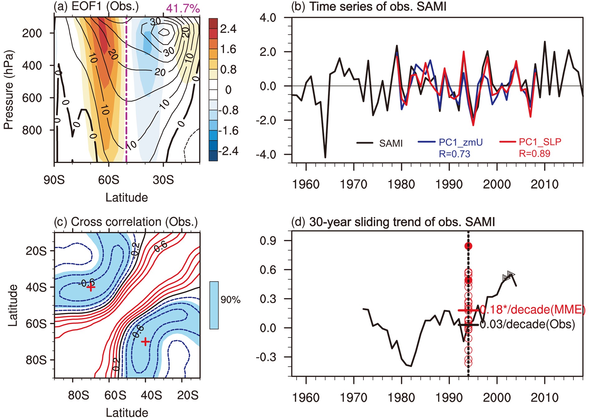 Figure1. The (a) EOF1 (shading; units: m s?1) and climatology (contours; units: m s?1) of zonal-mean zonal wind from reanalysis. The number in the top-right corner is the explained variance of EOF1. The purple dashed line marks the climatological position of the eddy-driven jet. (b) Time series of the observed SAMI proposed by Marshall (2003). Also shown are other definitions of the SAMI and their correlation coefficients with the SAMI-Marshall index during the period of interest (1979?2008). (c) Cross correlation of zonal-mean SLP among different latitudes (contours) from reanalysis, with the 90% confidence level shown by the shading. The cross symbols mark 40°S and 70°S. (d) The 30-year sliding trend of observed SAMI (black curve). The triangles indicate values significant at the 90% confidence level. For the period 1979?2008, the trends of the simulated SAMI from 28 models are shown as red circles. The solid and open circles indicate significant and non-significant values at the 90% confidence level. The red and black horizontal lines mark the MME and observed values for 1979?2008.
Models perform differently in simulating the JJA SAMI trend during 1979?2008. Specifically, 22 out of 28 models simulate a positive SAMI trend, and a negative trend exists in 6 models (Fig. 1d). The positive trend is significant at the 90% confidence level in GFDL-CM3 [0.49 (10 yr)?1] and GFDL-HIRAM-C180 [0.84 (10 yr)?1]. The strongest negative trend occurs in MPI-ESM-LR [?0.36 (10 yr)?1]. The intermodel standard deviation for the JJA SAM trend, 0.28 (10 yr)?1, is even larger than that of the multimodel ensemble (MME) [0.18 (10 yr)?1]. Figure 2a shows the time series of the SAMI from individual models and the MME. Two other definitions quantifying the temporal variability of the simulated SAM are also used for cross-validation. The correlation between SAMI and PC1_zmU and PC1_SLP are significant (Fig. 2a). The conditional MME (CMME; Yu et al., 2019) of the five models with the highest (lowest) SAMI trend is referred to as CMME1 (CMME2). CMME1 includes BCC-CSM1-1-M, EC-EARTH, GFDL-CM3, GFDL-HIRAM-C180, and MIROC5; CMME2 includes BNU-ESM, CCSM4, INMCM4, MPI-ESM-LR, and MPI-ESM-MR. Long-term changes in SAMI from CMME1 and CMME2 exhibit opposite trend (Fig. 2b). The trend from CMME1 is 0.33 (10 yr)?1 (significant at the 90% level), while that from CMME2 is ?0.19 (10 yr)?1 (significant at the 90% level). The distinction between CMME1 and CMME2 manifests the model difference in simulating the SAMI trend.
 Figure2. (a) Time series of the simulated SAMI from individual models (gray) and the MME (red). PC1_zmU (purple) and PC1_SLP (blue) are also shown. (b) Time series of the simulated SAMI from CMME1 (red) and CMME2 (blue). The dotted lines represent linear trend components. The pink and light-blue shading illustrate the model spread quantified by one standard intermodel deviation.
The trend in the zonal wind congruent with SAMI is obtained by first calculating the regression coefficients of the zonal wind on SAMI and then multiplying the result by the SAMI trend (Fig. 3). By doing this, the changes in SAMI are linearly projected on the zonal wind field. Observationally, the changes in zonal wind related to the SAM are relatively weak (Fig. 3a), because the observed SAMI trend is non-significant (Fig. 1d). In the models from CMME1 (Figs. 3b-f), the westerlies congruent with the SAMI variability strengthen in high latitudes, while those in middle latitudes weaken, implying a poleward shift of the westerlies. In contrast, the zonal wind trend congruent with SAMI generally shows opposite changes in the models from CMME2, i.e., it weakens in high latitudes but strengthens in middle latitudes, suggesting an equatorward shift of the westerlies (Figs. 3g-k). The differences between CMME1 and CMME2 are clearly evident (Fig. 3l). Also shown in Fig. 3 are linear trends in total zonal wind. Similar to the trend congruent with SAMI, the westerly jet shifts poleward in CMME1 but exhibits an opposite equatorward shift in CMME2. This is reasonable because the SAM accounts for a large portion of circulation variability in the extratropics, and model spread in simulating the SAMI trend contributes to model spread in simulating changes in extratropical circulation.
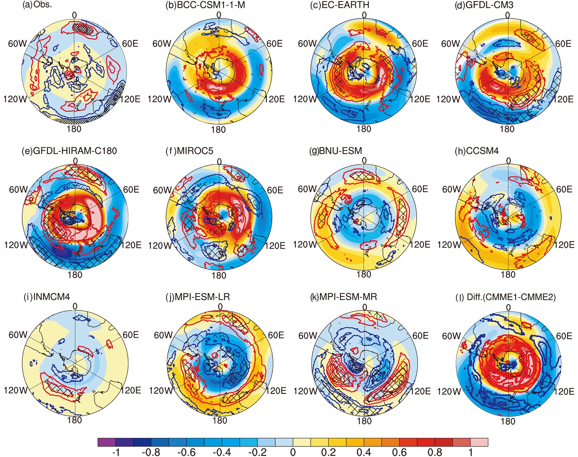 Figure3. Linear trend in vertically integrated tropospheric zonal wind [contours; units: m s?1 (10 yr)?1]. Red and blue contours show positive and negative values. The patches mark significance at the 90% confidence level. Also shown are the zonal wind trends congruent with SAMI [shading; units: m s?1 (10 yr)?1]: from (a) observations; (b?f) models in CMME1; (g?k) models in CMME2; and (l) the difference between CMME1 and CMME2.
To further investigate distinctions between CMME1 and CMME2 in simulated long-terms circulation changes, the differences in the linear trends of zonal-mean zonal wind (Fig. 4a) and geopotential height (Fig. 4b) are investigated. Accompanied by the poleward shift of the westerly jet, the polar vortex strengthens in CMME1. In contrast, the polar vortex weakens in CMME2. Statistical significance testing suggests the differences between the two groups are significant at the 90% confidence level.
 Figure4. (a) Difference in the linear trend of the zonal-mean zonal wind [units: m s?1 (10 yr)?1] between CMME1 and CMME2 (contours). Shading represents similar analysis but for the component in zonal wind congruent with SAMI [units: m s?1 (10 yr)?1]. Hatching indicates the difference is significant at the 90% confidence level. (b) As in (a) but for zonal-mean geopotential height [units: hPa (10 yr)?1].
In the next section, potential factors underlying model differences in the simulated SAMI trend are investigated from the aspect of extratropical SST.
4.1. Linkage between the SOD and SAM
The distribution of correlation between SST and SAMI from the MME exhibits a zonal symmetric characteristic to a certain degree (Fig. 5a), which is more evident in Fig. 5b. The correlation between zonal-mean SST and SAMI shows that the strongest positive and negative correlation locates at around 40°S and 60°S, respectively. In fact, this dipole-like SST anomalies pattern resembles the dominant mode of Southern Hemisphere extratropical SST, which is referred to as the SOD (Zheng et al., 2018). The spatial pattern of the SOD is quantified by EOF1 of SST and zonal-mean SST south of 30°S (Figs. 5c and d). The corresponding PC1s are referred to as PC1_SST and PC1_zmSST. The explained variance of the SOD for zonal-mean SST is about 50%. To conveniently quantify the temporal variability of this dipole-like SST anomaly pattern, a SOD index is defined as the difference in SST between 40°S and 60°S. The SODI and PC1_SST (PC1_SSTzm) are highly correlated, with a correlation of 0.82 (0.91) (Fig. 5e). Standardized time series of SODI and SAMI from the MME are shown in Fig. 5e. Covariability exists between SODI and SAMI, with a significant correlation of 0.42. Figure5. (a) Correlation between SST and SAMI from the MME (shading). (b) As in (a) but for zonal-mean SST (blue curve). Also shown is the partial correlation after removing the contemporaneous ENSO signal (black). The shading illustrates the model spread quantified by one standard intermodel deviation. (c) EOF1 of SST south of 30°S (units: °C). (d) EOF1 of zonal-mean SST south of 30°S (units: °C). (e) Standardized time series of SAMI from the MME (red) and SODI (blue solid), with their linear trend components shown as thin lines. The blue dashed and blue dotted lines are PC1_SST and PC1_zmSST. (f) Correlation between SODI and SAMI (ordinate) versus the correlation between inverted ENSO index and SAMI (abscissa).
ENSO plays a role in influencing the SAM (L’Heureux and Thompson, 2006; Gong et al., 2010). The partial correlation between the zonal-mean SST and SAM after linearly removing the contemporaneous ENSO is used to validate the linkage between the SST and SAM (Fig. 5b). Linearly removing ENSO slightly reduces the connection between the extratropical SST and SAM; the correlation remains significant at 40°S and 60°S. A model with good skill in simulating the ENSO?SAM relationship does not ensure a good performance in capturing the SOD?SAM relationship (Fig. 5f). Therefore, the perturbation form ENSO on the model-simulated SOD?SAM relationship is not considered in the following analysis.
2
4.2. Intermodel diversity related to the SOD
The correlation between the SST and SAMI from CMME1 is shown in Figs. 6a and b, in which the SOD structure is found: positive and negative correlation appear at around 40°S and 60°S, respectively. However, the dipole-like structure from CMME2 (Figs. 6c and d) shows an opposite phase: negative correlation exists at 40°S and positive correlation exists at 60°S. The difference between CMME1 and CMME2 is shown in Figs. 6e and f, illustrating that models with a higher SAMI trend (CMME1) are characterized by a stronger SOD?SAM connection.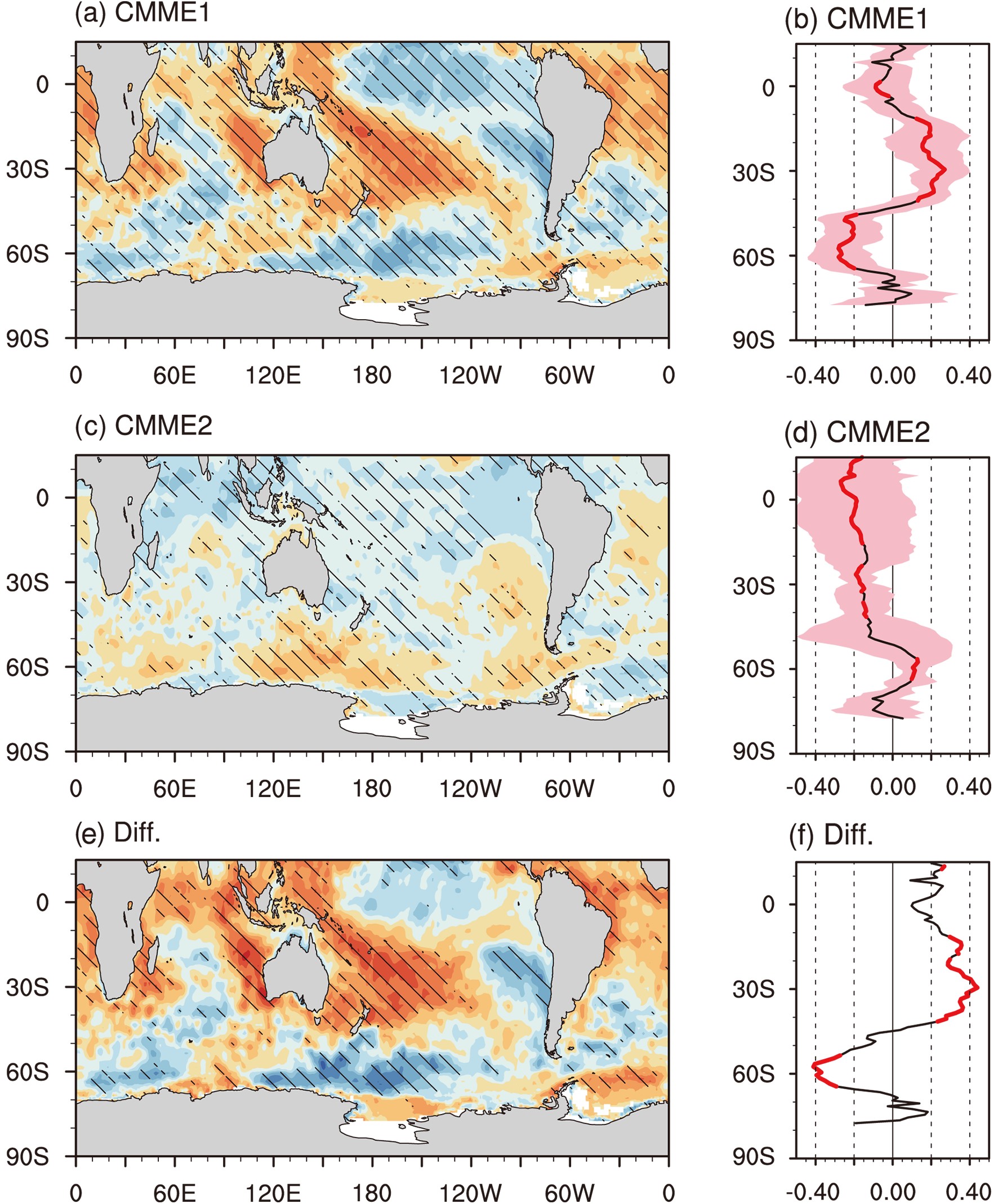 Figure6. Correlation between the SST and SAMI from (a) CMME1 and (c) CMME2. (b, d) As in (a, c) but for zonal-mean SST. Shading represents the intermodel spread quantified by one intermodel standard deviation. The patches in (a, c) and red curves in (b, d) indicate the locations where four out of five models have the same sign. (e, f) The difference between CMME1 and CMME2. The patches in (e) and red curves in (f) indicate the difference is statistically significant at the 90% confidence level.
The intermodel correlation between the SAMI trend and SST?SAMI relationship (Fig. 7a) is calculated as follows: (1) For a specific grid on the map, the intermodel correlation is calculated between two series: one series is the SAMI trend from 28 models; the other is the SST?SAMI correlation from 28 models. (2) Repeating this process at every grid, the distribution in Fig. 7a is then obtained. Note that the series of the SAMI trend is identical among the grids, but the series of the SST?SAMI correlation is grid-dependent. The stronger the SAMI trend, the higher (lower) the SST?SAMI correlation in middle (high) latitudes. That is, the stronger the SOD?SAM connection, the stronger the SAMI trend. The results for zonal-mean SST also suggest a dependence of the model-simulated SAMI changes on model skill in reflecting the SOD?SAM relationship (Fig. 7b). Also shown are results based on the other two SAM definitions, PC1_SLP and PC1_zmU. The consistency among the three curves suggests that the intermodel relationship in Fig. 7b is insensitive to the SAM definition.
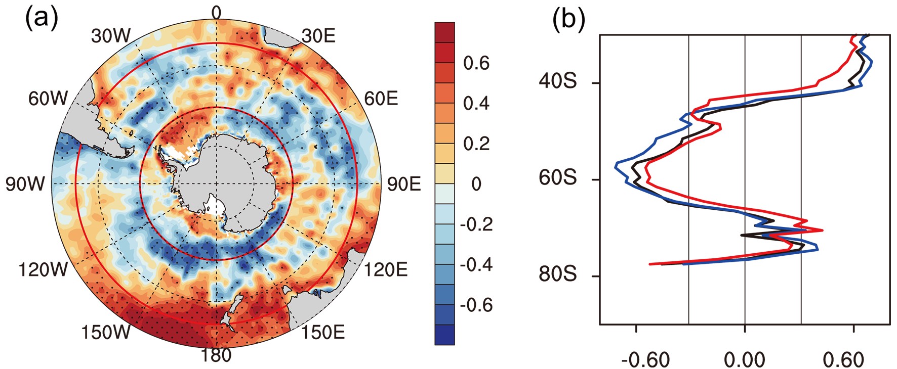 Figure7. (a) Intermodel correlation between the SAMI trend and SST?SAMI correlation. Stippling represents the 90% confidence level. (b) As in (a) but for the zonal-mean SST (black). The blue and red curves show results when the SAMI is replaced by PC1_SLP and PC1_zmU.
Figure 8a shows a scatter diagram of the trend in SAMI against the SOD?SAM relationship. The correlation between the ordinate and abscissa data is 0.69, implying model performance in simulating the SOD?SAM relationship accounts for 48% of the intermodel variance in simulating the SAMI trend. Conducting similar analysis using other SAMI definitions, the linkage between the simulated SOD?SAM relationship and SAMI trend is also clear. The explained variances using PC1_SLP (Fig. 8b) and PC1_zmU (Fig. 8c) are 55% and 30%, respectively. On average, model performance in simulating the SOD?SAM relationship accounts for about 40% of the intermodel variance in simulating the SAM trend in the AMIP runs.
 Figure8. (a) Scatterplot of the trend in SAMI (ordinate) against the SODI?SAMI correlation (abscissa). (b, c) As in (a) but the SAMI is replaced by (b) PC1_SLP and (c) PC1_zmU. (d) Intermodel correlation between the trend in SAMI and the trend in the meridional gradient of potential temperature. (e) Intermodel correlation between the trend in geopotential height and the SODI?SAMI correlation. Stippling marks the 90% confidence level.
Previous studies have found that the SOD plays a role in influencing extratropical circulation by influencing baroclinicity. Specifically, a positive SOD phase corresponds to increased (decreased) baroclinicity south (north) of 50°S. According to eddy?zonal mean flow interaction theory, anomalies in baroclinity tend to produce anomalous eddy momentum flux convergence (divergence) south (north) of 50°S, resulting in strengthened (weakened) westerly flow south (north) of 50°S, leading to a positive SAM phase (Zheng et al., 2015, 2018). Figure 8d shows the intermodel correlation between the SAMI trend and the trend in the meridional gradient of potential temperature, which is a measure of baroclinicity. A model with a stronger SAMI trend is characterized by stronger and weaker baroclinicity at around 60°S and 40°S, respectively.
The intermodel correlation between the trend in geopotential height and the SOD?SAM relationship shows that models with a closer SOD?SAM linkage tend to simulate a larger deepening trend of the polar vortex (Fig. 8e). Since deepening of the polar vortex is a manifestation of the increasing trend of SAMI, Fig. 8 further verifies that the simulated influence of the SOD on the SAM acts as one source of model spread in depicting long-term changes in the SAM.
Using AMIP simulations from 28 models archived in CMIP5, this study shows that the intermodel diversity in the trend of the austral winter (JJA) SAMI is non-negligible, with the intermodel standard deviation of 0.28 (10 yr)?1 being larger than the MME of 0.18 (10 yr)?1. The model spread in simulating the SAMI trend contributes to the model spread in depicting the changes in extratropical circulation. The polar jet shifts toward the Antarctic and the polar vortex strengthens in models with significant positive SAM trend, while in models with significant negative SAM trend, polar jet exhibits equatorward shift and polar vortex weakens. The differences between the two groups are significant.
The role of SOD-like SST anomalies in influencing the SAM is found in AMIP simulations, which is consistent with previous studies (Liu et al., 2015; Zheng et al., 2015). Model performance in simulating the SAMI trend is linked with model skill in reflecting the SOD?SAM relationship. Models with stronger correlation between the SOD and SAM tend to simulate a stronger SAM trend, and vice versa. Model performance in simulating the SOD?SAM relationship accounts for about 40% of the intermodel variance in simulating the SAM trend in the AMIP runs. The ability of models in depicting internal processes of the climate system acts as one source of model uncertainty in simulating the response of the climate to external forcing. The above result is a manifestation of the fact that the direct effect of external forcing on climate changes might be influenced by internal processes in the climate system (Cane et al., 1997).
Focusing on the responses of atmospheric circulation to SST anomalies, this study only used AMIP models. In the real climate system, there is a two-way coupling between the atmosphere and ocean, i.e., the SAM also plays a role in influencing the SOD (e.g., Wang and Fan, 2005; Sen Gupta and England, 2006; Fan, 2007; Yang et al., 2007; Bian et al., 2010; Shi et al., 2013; Wu and Francis, 2019; Wu et al., 2020; Yuan et al., 2020). Using atmosphere?ocean coupled experiments to verify the contribution of SOD?SAM coupling to model uncertainty helps in further understanding the reasons underlying the intermodel diversity. As outputs from CMIP6 have become available, the relationship between the simulated SAM trend and model performance in capturing the SOD?SAM relationship needs to be further validated using these latest models.
Aside from the extratropical SOD, tropical SST anomalies (e.g., ENSO) also plays a role in influencing the SAM variability. The teleconnection from lower latitudes exhibits seasonal features. Investigating the seasonality of the SOD?SAM relationship in further study will be helpful for understanding extratropical air?sea interactions. Furthermore, whether the role of the SOD?SAM relationship in influencing the SAM trend is seasonally dependent remains an open question.
Acknowledgements. This work was jointly supported by the Strategic Priority Research Program of the Chinese Academy of Sciences (Grant No. XDA19070402), a National Key Research and Development Project (Grant No. 2018YFA0606404), and the National Natural Science Foundation of China (Grant Nos. 41790474 and 41775090). We acknowledge the World Climate Research Programme’s Working Group on Coupled Modelling, which is responsible for CMIP, and we thank the climate modeling groups for producing and making available their model output. The authors appreciate the comments of the two anonymous reviewers and the editor.
