王飞^,1,2,3, 杨胜天², 魏阳², 杨晓东^2,3, 丁建丽^,1,2,31 新疆大学智慧城市与环境建模新疆普通高校重点实验室,乌鲁木齐830046
2 新疆大学资源与环境科学学院,乌鲁木齐 830046
3 绿洲生态教育部重点实验室,乌鲁木齐 830046

Influence of Sub-Region Priority Modeling Constructed by Random Forest and Stochastic Gradient Treeboost on the Accuracy of Soil Salinity Prediction in Oasis Scale

WANG Fei^,1,2,3, YANG ShengTian², WEI Yang², YANG XiaoDong^2,3, DING JianLi^,1,2,3 1 Xinjiang Common University Key Laboratory of Smart City and Environmental Stimulation, Xinjiang University, Urumqi 830046
2 College of Resource and Environmental Sciences, Xinjiang University, Urumqi 830046
3 Laboratory for Oasis Ecosystem, Ministry of Education, Urumqi 830046

通讯作者: 丁建丽,E-mail：dingjianlixjdx@126.com

第一联系人: 王飞,E-mail： volitation610@163.com。
收稿日期:2018-05-14接受日期:2018-07-20网络出版日期:2018-12-26

基金资助:

国家自然科学基金.U1603241、41661046、41771470、41261090、U1303381 新疆大学博士研究基金.BS150246

Received:2018-05-14Accepted:2018-07-20Online:2018-12-26


摘要
目的 试图通过优先在干旱区绿洲的子区构建模型以提高绿洲全局土壤盐度的预测精度。同时量化全局模型和子区模型之间精度的差异性和不确定性。方法 利用随机森林（Random Forest,RF）和随机梯度增进算法（Stochastic Gradient Treeboost,SGT）定量化上述不确定性,同时,对比本地尺度多个情景(景观)优先建立模型再合并预测值对于模拟全局土壤盐度的精度影响。基于驱动因子（土地利用和地貌）,响应因子（Normalized Difference Vegetation Index, NDVI和土壤电导率,EC）,研究设计了27个能够相对覆盖典型绿洲不同土壤盐度变异性的环境情景。结果 70.37%（19/27）的情景证明SGT的预测精度高于RF。单独建模的10个情景的预测精度高于全局模型下10个再分类情景（根据情景设定规则将全局模型预测值再分类）的精度。特别是,EC≤4 dS·m ^-1 和 2 dS·m ^-1＜ EC＜16 dS·m ^-1两个情景应该单独进行建模预测。4个情景（两两合并）预测值合并后的精度高于全局模型再分类后的精度。需要指出的是,用于绿洲尺度子区情景构建的首选分割变量是EC,其次是地貌和土地利用。结论 研究推荐基于SGT在绿洲内部不同景观尺度上优先建模,再将各景观尺度的预测值进行合并,以提高绿洲土壤盐度的推理精度。
关键词： 土壤盐分;机器学习;干旱区;Landsat OLI;空间异质性;随机森林算法;随机梯度增进算法

Abstract
【Objective】 This study attempts to improve the prediction accuracy of soil salinity in arid oasis by building models preferentially in the sub-area of oasis. At the same time, the difference and uncertainty of accuracy between global model and sub-region model are quantified. 【Method】 Therefore, to investigate the above differences, this study used two machine learning methods (Random Forest, RF and Stochastic Gradient Treeboost, SGT) to quantify the above effects and to prove the necessity of the building model in the sub-region compared with the full-sample model with respect to the simulation precision under the complex background of an arid region. Twenty-seven environmental scenarios (twelve original and fifteen derivatives) were designed based on the driving factors (land use and landform) and response factors (Normalized Difference Vegetation Index, NDVI and electrical conductivity, EC), which reflected variety of variabilities in soil salinity. After analyzing the results, the following preliminary conclusions were drawn. 【Result】 The simulation results from 70.37% (19/27) of the scenarios showed that the predicted value of soil salinity from SGT was closer to the observed value from RF. Ten original sub-regions were modeled individually and compared with the full-sample model under the oasis scale (according to the 10 partition rules to reclassify the simulated values), and the result showed that the prediction accuracy of the former 70% scenario was higher than that of the latter. In particular, the regions of EC≤4 dS·m ^-1 and 2 ddS·m ^-1＜EC＜16 dS·m ^-1 should be modeled separately to predict the spatial variability of regional salinity. By combining the predictions of sub-regions and comparing them with the predicted values of the full-sample model, the former (all four different combination modes) showed a higher prediction accuracy than the latter. In addition, this result also indicated that the preferred medium for partitioning the sub-regions was soil electrical conductivity, followed by landform and land use. 【Conclusion】 The study proposes to establish a soil salinity model based on SGT preferentially on different landscape scales within the oasis, and then combine the predicted values of each landscape scale to improve the prediction accuracy of oasis soil salinity.
Keywords：soil salinity;machine learning;arid regions;Landsat OLI;spatial heterogeneity;Random Forest;Stochastic Gradient Treeboost


PDF (11238KB)元数据多维度评价相关文章导出EndNote|Ris|Bibtex收藏本文
本文引用格式
王飞, 杨胜天, 魏阳, 杨晓东, 丁建丽. 基于RF和SGT算法的子区优先建模对绿洲尺度 土壤盐度预测精度的影响[J]. 中国农业科学, 2018, 51(24): 4659-4676 doi:10.3864/j.issn.0578-1752.2018.24.007
WANG Fei, YANG ShengTian, WEI Yang, YANG XiaoDong, DING JianLi. Influence of Sub-Region Priority Modeling Constructed by Random Forest and Stochastic Gradient Treeboost on the Accuracy of Soil Salinity Prediction in Oasis Scale[J]. Scientia Agricultura Sinica, 2018, 51(24): 4659-4676 doi:10.3864/j.issn.0578-1752.2018.24.007

0 引言

【研究意义】土壤盐渍化的精准预测是评估绿洲生态环境的适应性和提高资源利用效率的重要前提。【前人研究进展】已有诸多基于遥感信息识别不同区域土壤盐渍化影响程度和分布范围的研究^{[1,2,3,4,5,6,7,8]}。以上研究基于不同传感器（IKONOS,Landsat, MODIS）获取的数据,计算与土壤盐度相关的指数,并建立全局土壤盐度模型,成功预测了各自研究区内盐渍化土壤的分布范围。【本研究切入点】然而,绿洲尺度下与土壤盐分呈现响应关系的环境变量是否可以在绿洲景观组分内（如土利用类型、地貌类型、不同植被覆盖度）持有同等显著性的空间变异解释力尚不明确。绿洲内影响陆气水热交换的因素（如地表粗糙度、反照率）随着自然生境向人工灌溉农业的转变发生改变^[9],致使不同土地利用类型之间表面能量和净辐射量发生变化^[10]。绿洲内环境建构组分如不同土地利用类型（农田、灌木、草地、盐碱地等）对水盐运移的驱动机制也各有不同^[11,12,13]。若仅依靠全局尺度建构的土壤盐渍化-环境变量模型模拟组分内的土壤盐度空间变异性,可能存在值域被夸大或被低估,甚至被误判的现象（基于流域/绿洲尺度选择的环境变量可能无法充分解释组分内部相对均匀环境中的土壤盐度变化）^[14,15]。组分尺度（农田、灌木、草地、盐碱地等）上对于土壤盐渍化-环境响应关系精确定量描述可能有助于提高绿洲尺度的土壤盐渍化制图精度。统计学方法是土壤盐渍化定量研究中的重要手段。机器学习被定义为基于现代统计方法挖掘目标和响应变量之间关系模式的过程^[16]。通过查找文献,随机森林（Random Forest, RF）和随机梯度增进算法（Stochastic Gradient Treeboost, SGT） 是目前土壤制图领域应用较为广泛的机器学习方法^{[17,18,19,20]}。RF的优势在于具备非线性挖掘能力;数据分布不需要符合任何假设;同时处理类型和连续变量;防止过度拟合;有效抑制数据中存在的噪声;定量描述变量的贡献度;只需要率定少量参数^[21]。SGT由CART改进而来,通常可以实现准确和稳健的预测,有效抑制过度拟合效应^[22]。不需要变量的先验假设,比传统的广义线性或加权模型提供更大的灵活性。存在空间异质性和异常值时,SGT依然能获得较高的预测精度。在复杂关系定义的干旱区土壤生态系统,上述算法具备的优势显得尤为重要。然而,这两种优秀的现代统计学算法鲜有用于预测干旱区土壤盐度的先例。【拟解决的关键问题】本研究一是比较不同环境建构组分下RF和SGT的预测能力;二是定量化描述绿洲分区建模对绿洲尺度盐度预测精度的影响;三是获取不同环境建构组分条件下的敏感因子及其贡献度。

1 材料与方法

1.1 研究区

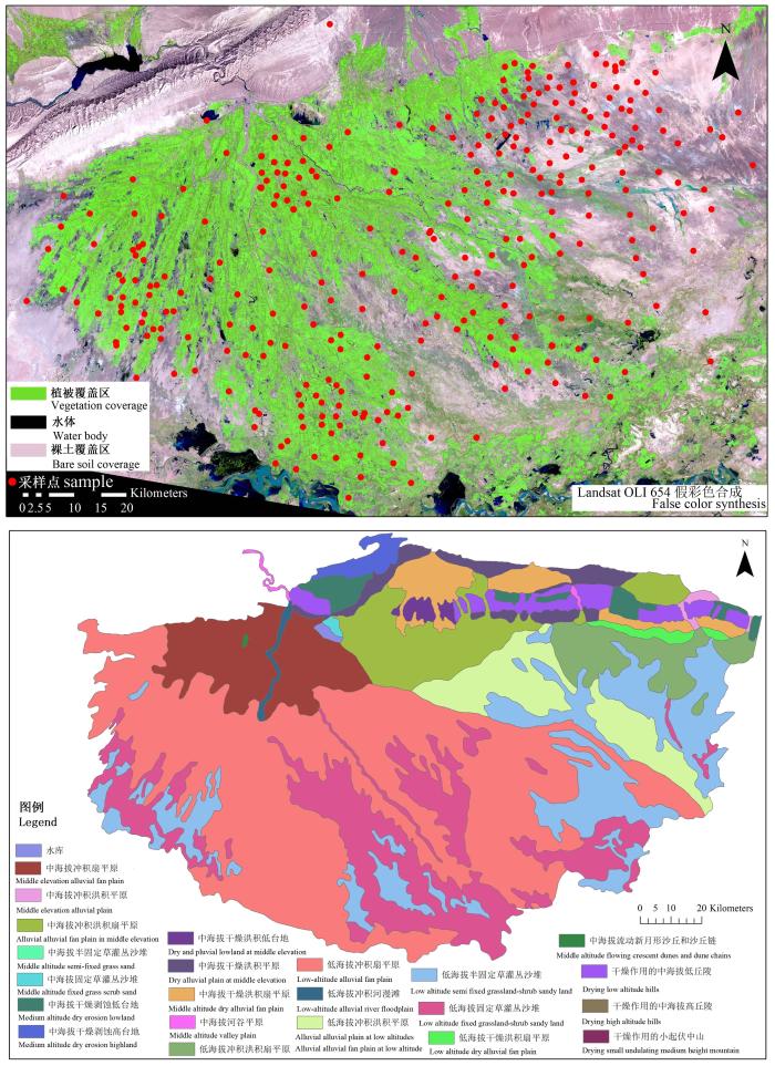
渭干河-库车河流域（渭库）是位于塔里木盆地北部的一个典型绿洲。该研究区的中心经纬度坐标为82.50°N,41.38°E,主要地貌类型有：低海拔冲积扇平原、低海拔冲积平原、中等高度冲积扇平原、低海拔固定草灌木区,以及低海拔半固定草灌木区（图1）。研究区海拔范围为892—1 100 m,从西北到东南逐渐降低。该区主要的土壤类型为：积土成土、盐碱土、石膏层/钙盐土、钙积变性土、钙成土和石灰性黑土。灌区外围受土壤盐渍化和土壤水分的影响,整体的植被覆盖度较低,自然植被主要包括：Phragmites australis, Tamarix ramosissima, Alhagi sparisifolia, Karelina caspica, and Kalidium gracile^[23]。该区为极端干旱荒漠气候,年平均降雨量为51.6 mm,年平均蒸散量为2 356 mm,年积温为（＞ 10℃）为4 500℃。由于水库引水灌溉急剧增加（由于灌溉土地的扩张）,该区地下水位和地下水矿化度显著增加。地下水位上升和地下水盐化是造成土壤盐渍化的主要因素^[24]。耕地盐渍化面积超过50%,其中30%的耕地受到严重影响^[25]。

图1

新窗口打开|下载原图ZIP|生成PPT
图1渭干河-库车河流域景观地貌特征及绿洲采样点分布图

Fig. 1Distribution of the field sampling plots at Weigan-kuqa river oasis

1.2 数据与方法

1.2.1 土壤样品采集与土壤盐分分析处理 为了进行土壤盐度分析和建模预测,本研究共计获得了371个样本。根据实际情况最终样点的布局采取两种不同的设计方式,采样点分布情况见图1。研究初步的样点布局是基于限制拉丁超立方体（Conditioned Latin Hypercube Method,cLHS）而设计^[26]。该方法是在已确定采样数目的前提下抽取尽可能全面地覆盖由定性或定量变量构成的属性空间的样本。cLHS的程序和算法可在Minasny和McBratney（2006）文献中可以找到。然而,在实际采样中,由于各种原因（道路不通、植被过密或地形崎岖）,3/5的位置未能被抵达。因此,我们随后采用了分层随机抽样的策略,样点的布局综合考虑了绿洲景观类型、水文特征、道路通达性和土壤盐渍化空间异质性、土地利用和地形等因素。数据收集时间为2016年9月9—30日。每个样点用五点梅花的方式取土,采样深度为0—10 cm,随后将测试的数据进行平均,作为本样点的实际观测值。

本研究中,土壤盐度（测定土水比1﹕5溶液电导率,EC_1:5）在实验室内进行分析,参照《土壤和农业化学分析》,将土样风干后磨碎,过2 mm筛子,制备土壤溶液,比例为土水比1﹕5,温度设定为25℃,用以测定土壤样本的电导率（EC _1:5）^[27]。所有样点的电导率平均值作为采样点的基本值。此外,本研究区EC _1:5和土壤盐分（g·kg^-1）具有高度相关性（R² = 0.95）,所以EC_1:5可用作评估研究区土壤盐分的替代参数。

1.2.2 Landsat OLI图像预处理 本研究所使用的卫星影像是Landsat OLI（145/31）,获取时间为2016年9月18日。基于ENVI 5.3中的FLAASH（Fast line- of-slight Atmospheric Analysis of Spectral Hypercubes）模型纠正大气带来的影响。纠正后的反射率数据,其数值范围为0—1。该数据用于计算后续研究中使用的各类土壤或植被相关指数。

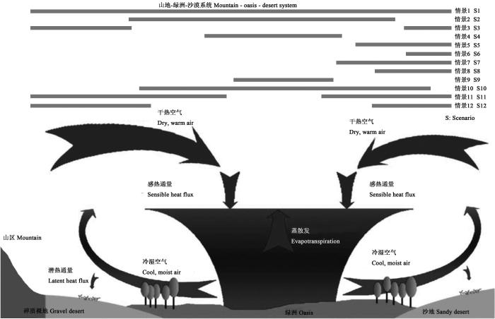
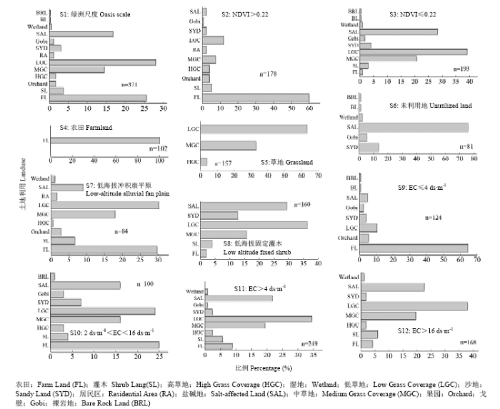
1.2.3 基于驱动和响应因子的场景设计 本研究基于驱动因子和环境响应因子,设定以下12个场景用以量化分区建模对于绿洲尺度土壤电导率预测精度的影响（图2）。将绿洲尺度的全部样本构建的模型设置为情景1。基于植被覆盖情况,将植被覆盖程度分为全覆盖（NDVI＞0.22,情景2）和无植被覆盖（NDVI≤0.22,情景3）。NDVI阈值（0.22）的设定参考WU 等^[5]和 SONG 等^[28]的研究成果;基于土地利用：农业用地（情景4）、草地（情景5）和未利用土地（情景6）;基于地貌：低海拔的冲积扇平原（情景7,LAAFP）和低海拔固定灌木（情景8,LAFGS）;基于土壤电导率分级（EC）^[29]：EC ≤ 4 dS·m^-1（情景9）,2 dS·m^-1＜EC＜16 dS·m^-1（情景10）,EC＞4 dS·m^-1（情景11）,EC＞16 dS·m^-1（情景12）。场景的设置同时考虑了土壤发生学和人类活动影响。此外,研究还想说明分层预测非均质地表土壤电导率的重要性。图3显示了每个场景的土地利用类型的组成。

图2

新窗口打开|下载原图ZIP|生成PPT
图2绿洲-沙漠水热和能量交换示意及情景覆盖范围（修改自LI等^[10]）

Fig. 2Schematic diagram of the interactions of hydrothermal and energy exchange between oasis and desert areas as well as the relative coverage of each scenario (modified from LI et al^[10])

图3

新窗口打开|下载原图ZIP|生成PPT
图312个情景的土地利用分布特征

Fig. 3Statistical histogram of the land use types of the samples in the 12 scenarios



1.2.4 环境变量 基于土壤方程选择用于预测土壤电导率的环境变量：气候因子（地表温度）、生物因子（植被指数）、DEM（数字高程模型）衍生变量集（30、60、90、120、150、180、210和240 m等8个分辨率）、母质（地貌类型）、人类活动（土地利用）、土壤相关因子（波段、土壤相关指数、土壤湿度指数）。具体变量详见表1。

Table 1
表1
表1基于Landsat OLI（30 m）和DEM（8个空间分辨率）衍生的环境变量
Table 1Environmental covariates derived from a 30 m spatial resolution DEM and 30 m Landsat imagery

变量组 Environment variable group	指数 Index
波段及其衍生变量 Band & derivatives	全波段;缨帽变换（亮度（TC1）,绿度（TC2）,湿度（TC3）,主成分分析（前三个波段） Bands;Tasseled Cap (brightness,TC1;Greenness,TC2; Wetness,TC3 ), Principal Component Analysis(PC1,PC2,PC3)
植被指数 Vegetation indices	归一化植被指数;土壤调节植被指数;增强植被指数;广义植被指数;冠层响应盐度指数[3];比值植被指数;两波段增强植被指数[30];扩展的归一化植被指数[31];扩展的增强植被指数[31] Normalized Difference Vegetation Index, NDVI; Soil Adjusted Vegetation Index, SAVI; Enhanced Vegetation Index, EVI; Generalized Difference Vegetation Index, GDVI[5]; Canopy Response Salinity Index, CRSI[3]; Simple Ratio Vegetation Index, SR; Two-Band Enhanced Vegetation Index, EVI2[30]; Extended NDVI, ENDVI[31]; Extended EVI, EEVI[31]
土壤相关指数 Soil-related indices	盐度指数（Salinity Index, SIT）[1];盐度指数（Salinity Index, SI）[1];盐度指数（Salinity Index（SI1）[1];盐度指数（Salinity Index, SI2）[1];盐度指数（Salinity Index, SI3）[1];盐度指数（Salinity Index, SIA）[1];盐度指数（Salinity Index, SIB）;盐度比值指数（Salinity Ratio, SAIO）[32];黏土指数（Clay Index, CLEX）[4] ;石膏指数（Gypsum Index, GYEX）[4];亮度指数（Brightness Index, BREX）[4];碳酸盐指数（Carbonate Index, CAEX）[4];FSEN= (B5-B7）/(B5+B7）[33];颜色指数（Color Indices -色相Hue, 饱和度 Saturation, 色调Value）;归一化热感指数（Normalized Difference Infrared Index, NDII）[4];全球植被湿度指数（Global Vegetation Moisture Index, GVMI）[34];地表温度（Temperature）
DEM衍生因子 Dem derivatives	河道相关：谷深（Valley Depth ,VD）;与河网的垂直距离（Vertical Distance To Channel Network ,VDCN）;水文学相关：坡长因子（LS-Factor, LSF）;地形指数指数（Topographic Wetness Index, TWI）;坡长（Slope Length, SL）;通视度（Sky View Factor, SVF）;地形位置指数（Topographic Position Index, TPI）;多尺度谷底平整度（Multiresolution Index Of Valley Bottom Flatness（MRVBF And MRRTF））,坡高（Slope Height, SH）,归一化高度（Normalized Height, NH）,标准化高度（Standardized Height, STH）,坡度中值位置Mid-Slope Position（MSP）,地表纹理（Terrain Surface Texture, TEX）,汇流累积量（Flow Accumulation, FA）;形态：截面曲率（Cross-Section Curvature, CSC）,纵向曲率（Longitudinal Curvature, LC）,相对坡度位置（Relative Slope Position, RSP）,流域坡度（Catchment Slope, CS）（SAGA Development Team, 2011）

新窗口打开|下载CSV

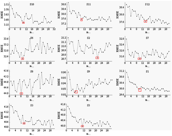
1.2.5 RF & SGT RF模型是基于决策树发展而来的一种集成学习方法,通过多次 bootstrap抽样获得多个随机样本,并通过这些样本分别建立相对应的决策树,从而构成随机森林。用于回归的 RF,取所有决策树预测结果的均值作为最终的预测结果^[21]。RF算法主要涉及两个关键参数：一是对于每个参与模型的分支树,即模型运算中的分裂次数m_try的设定。参与预测的变量个数不同,m_try的设定也不同,需要根据实际情况调整。本文针对设置的12个情景分别定义m_try。研究根据RF模型预测过程中（63%的样本用于建模）产生的袋外误差（37% 的样本用于验证）对m_try的值再做具体的调整。每个情景的m_try值由1到30分别进行测试,取袋外误差最小的m_try值作为本情景最适宜的分裂次数。另一个是树模型运算中每次生成的树的数量,ntree,模型的计算量与 ntree的值成正比,在 ntree增加并不能显著提高模型预测能力的情况下,ntree的设定要尽可能小（一般＞500）,本文设定为1 000。RF模型的预测通过R语言的random forest工具包（randomForest）实现^[35]。

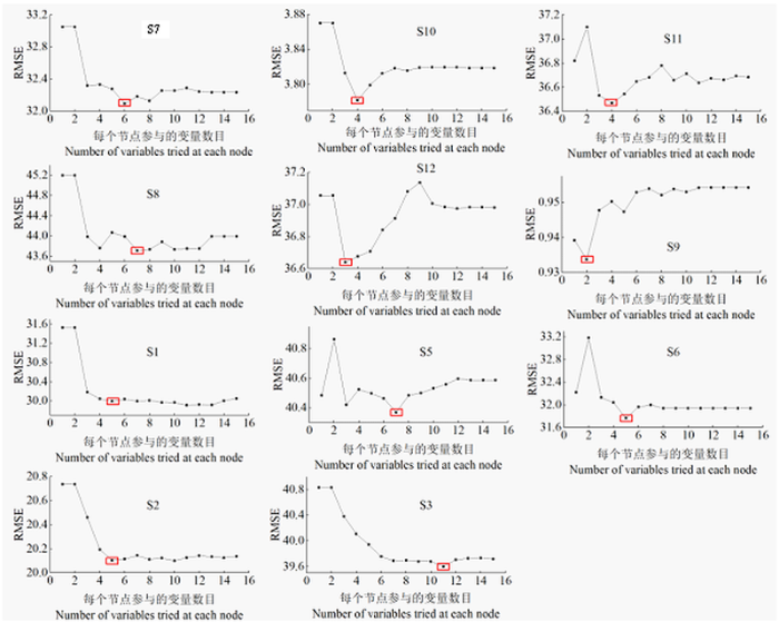
SGT是回归树和Boosting的集成。Boosting的核心思想是：初始状态下为每个训练样本赋予一样的权重值,每次迭代训练提高错分样本的权重,降低分对样本的权重。迭代N次之后,得到N个弱分类器,最终通过权重加和的方式集合成强分类器^[36]。SGT是Boosting算法框架的分支,该算法为了减少上次结果的残差,在减少残差梯度方向上不断建立新的模型,直到误差不在降低为止。该算法需要设置以下四个参数：学习速率,抽样比例,树的最大化子节点个数和每次生成的树的数量。学习速度越低,迭代次数越多,一般小于0.1,此研究中设置为0.01^[36]。抽样比例为1时,每次迭代的样本集相同,小于1时,抽取的训练样本集都不同,有助于抑制过拟合,取值范围0.5—0.8^[17],为了和RF进行对比,这里设置为0.63。树的最大化子节点个数需要根据实际情况设定,测试值的范围1—15,取RMSE最小的值为最佳最大化子节点个数（图6）。每次生成的树的数量设置为1000。

1.2.6 变量筛选与最佳组合的选择 研究表明通过去除潜在不相关的环境变量会提升模型的鲁棒性。原因在于筛选过程可不断降低不相关性的变量对模型精度的负向扰动,以提高预测的准确性。本研究会在以上12种情景下分别进行最佳变量组合的测试。筛选步骤主要参考SVETNIK等^[37]和HEUNG等^[18]的研究成果。（1）基于RF和SGT,对变量的重要性进行排序。（2）依次删除排在末尾最不重要的变量,并再进行迭代运算,验证采用5-fold交叉验证获取RMSE。根据RMSE最低值确定最佳变量组合。（3）在各个设定的情景中重复步骤1和步骤2,确定每个场景的最优变量组合。

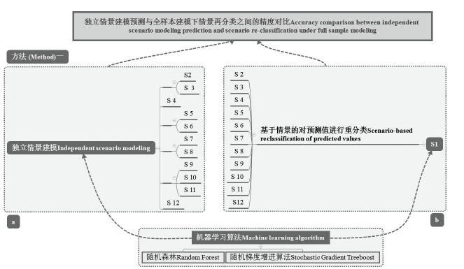
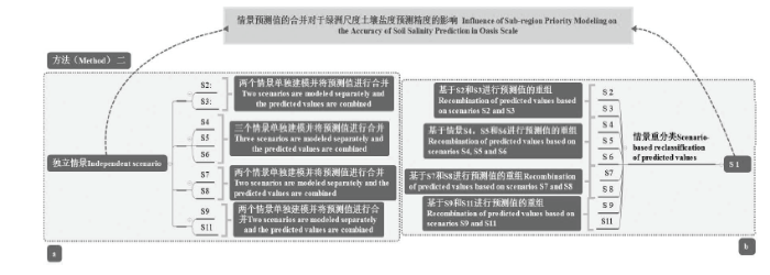
1.2.7 情景对比方案 研究采用以下两种方法比较情景（子区）重组对绿洲尺度盐度预测的影响。方案一基于全样本构建绿洲尺度预测模型,之后将预测值依据12个情景的设定规则重新组合（Regroup Scenarios,RS）（图4-b）。另外,为了对比,如图4-a所示,在12个情景中单独建立预测模型（Independent Scenarios,IS）。将上述两种模式生成的情景验证结果进行对比。方案二则组合不同场景的预测值,即NDVI＞0.22 & NDVI≤0.22,EC≤4 dS·m^-1& EC＞4 dS·m^-1,农用地,草地&未使用的土地, LAAFP & LAFGS,然后比较上述组合方案（Combined Scenarios,CS）（图5-a）与全样本预测值根据上述组合方式形成对应组合（Reclassified Scenarios from Oasis Scale Model,RSOSM ）的精度差异性（图5-b）。

图4

新窗口打开|下载原图ZIP|生成PPT
图4独立情景建模与全样本建模下预测值根据情景重分类之间的精度对比方案

Fig. 4Comparison of combined and regrouped scenarios on predictions of soil salinity in method one at oasis scale

图5

新窗口打开|下载原图ZIP|生成PPT
图5情景预测值的合并对于绿洲尺度土壤盐度预测影响的对比方案

Fig. 5Comparison of combined and regrouped scenarios on the prediction of soil salinity in method two at the oasis scale

1.3 模型评估

研究基于5折交叉验证（5-fold cross validation）获取各情景下最优模型并进行验证。此验证测试过程相对于简单的训练-验证比例而言需要花费更多的计算工作量,并适用于较小的数据集,结果可靠且具备无偏性^[17]。训练数据集被随机分成5个子集, 即4/5 的训练数据被用于模型训练,剩下的1/5用于模型验证。每个抽样过程重复20次,取其平均值。图6和图7显示了每个情景下经过4/5训练数据获取的RF算法中m_try的最优值（黑色放框）和 SGT算法中的最大化子节点个数的最优值（黑色放框）。研究采用相关系数 （R²）、均方根误差（Root Mean Square Error,RMSE） 和预测偏差比 （Residual Predictive Deviation,RPD） 作为误差评价指标。RMSE 越接近零,RPD 值越大,预测精度越高。

2 结果

2.1 土壤盐度变异性

表2显示了不同情况下土壤盐分的基本统计信息。情景1的统计分析表明, 该区土壤电导率最大值为 184.5 dS·m^-1,最小为 0.14 dS·m^-1,平均为 31.32 dS·m^-1。根据美国盐度实验室的盐度分类标准（0—2 dS·m^-1 为非盐渍化;2—4 dS·m^-1 为轻度盐渍化;4—8 dS·m^-1为中度盐渍化;8—16 dS·m^-1为重度盐渍化;＞16 dS·m^-1为极端盐渍化）,约67% 的样品（EC＞4 dS·m^-1）受到土壤盐渍化的影响。整体而言,不同情景的变异系数（coefficient of variation,CV）表明,该区0—10 cm土层的土壤盐度呈现中度或高度空间变异性。（CV＜0.1为低变异性,0.1＜CV＜1.0为中度变异性,CV＞1.0为高度变异性）。

图6

新窗口打开|下载原图ZIP|生成PPT
图6不同情景RF算法中m_try的最优值

Fig. 6The effects of the m_try set in RF on RMSE in different scenarios

图7

新窗口打开|下载原图ZIP|生成PPT
图7不同情景下SGT算法中最大化节点（node）的最优值

Fig. 7The effects of the maximum nodes per tree set in SGT on RMSE in different scenarios



Table 2
表2
表212个情景的土壤电导率（dS·m^-1）统计特征
Table 2Summary statistics of salinity (dS·m^-1) for the 12 scenarios used in this study

情景 Scenario	最小值 Min	最大值 Max	平均值 Average	变异系数 CV	Q25	Q50	Q75
S1	0.14	184.5	31.32	1.29	1.42	13.11	48.00
S2	0.14	128.50	11.25	2.02	0.42	1.50	9.90
S3	0.15	184.50	47.14	0.95	11.84	26.00	79.95
S4	0.15	103.9	5.57	2.97	0.38	0.90	3.36
S5	0.14	184.50	47.33	0.95	11.59	26.00	88.00
S6	0.23	150.50	34.38	1.10	6.76	17.33	60.90
S7	0.27	184.50	50.40	0.92	11.77	35.40	78.82
S8	0.14	147.40	28.20	1.37	1.34	10.69	33.89
S9	0.14	3.99	0.99	0.95	0.33	0.55	1.41
S10	2.01	15.92	8.47	0.50	4.54	7.97	12.04
S11	4.06	184.50	46.43	0.90	13.11	25.70	75.60
S12	16.28	184.5	64.10	0.63	24.85	61.10	94.15

新窗口打开|下载CSV

2.2 RF和SGT在土壤盐度预测中的表现

表3和表4分别显示了RS和IS模式下基于RF和SGT计算获取的误差水平。根据R²,RMSE 和 RPD的统计结果：（1）RF和SGT在情景2、3和5中的预测水平相似。（2）70%的情景中（情景2、3、5、6、7、8、11和12）,SGT的预测精度高于RF。R²依次增加了6.06%、0、5.13%、23.40%、-4.00%、51.52%、18.75% 和 16.67%。RMSE依次降低了2.21%、0.005%、1.47%、11.73%、16.14%、12.49%、3.79%和3.20%。RPD值依次增加了0.44%、0、1.56%、13.67%、18.80%、13.82%、4.10%、3.33%。RF在情景9和10的预测精度高于SGT,R²值提高了26.09%和34.21%。RMSE的值降低了4.82%和11.18%。RPD值增加了5.26%和12.50%。（3）所有情景的预测精度水平P＜0.01。表4的结果显示：（1）除了情景2,其余情景的RF和SGT的预测精度水平相似。情景2中,相对于RF,SGT的R²值增加了46.67%,RMSE降低了11.61%,RPD值增加了13.56%。（2）50%的情景显示SGT的预测精度高于RF。全样本模式下,SGT的预测精度高于RF。另外,由于农田样本的高变异性,RF和SGT都无法完成预测。

Table 3
表3
表3独立情景下（IS模式）基于随机森林和随机增进算法的精度验证
Table 3Validation statistics for RF and SGT to predict surface soil salinity for different independent scenario in Fig. 4a

情景 Scenario	随机森林 Random Forest			随机梯度增进算法 Stochastic Gradient Treeboost
	R2	RMSE	RPD	R2	RMSE	RPD
S2	0.33**	18.52	1.23	0.35**	18.11	1.26
S3	0.34**	36.487	1.23	0.34**	36.485	1.23
S4	0.39**	35.36	1.28	0.41**	34.84	1.30
S5	0.47**	27.36	1.39	0.58**	24.15	1.58
S6	0.50**	33.15	1.17	0.48**	27.80	1.39
S7	0.33**	37.88	1.23	0.50**	33.15	1.40
S8	0.29**	0.79	1.20	0.23**	0.83	1.14
S9	0.51**	2.94	1.44	0.38**	3.31	1.28
S10	0.32**	34.57	1.22	0.38**	33.26	1.27
S11	0.30**	34.08	1.20	0.35**	32.99	1.24

**: P＜0.01

新窗口打开|下载CSV

Table 4
表4
表4RS模式基于随机森林和随机增进算法的精度验证（根据情景划定规则重分类）
Table 4Validation statistics of RF and SGT to predict surface soil salinity for different scenarios originating at the oasis scale according to Method 1 in Section 1.2.7 in Fig. 4-b

情景 Scenario	随机森林 Random Forest			随机梯度增进算法 Stochastic Gradient Treeboost
	R2	RMSE	RPD	R2	RMSE	RPD
S1	0.46**	29.65	1.37	0.48**	29.17	1.39
S2	0.30**	19.20	1.18	0.44**	16.97	1.34
S3	0.38**	35.50	1.27	0.37**	35.71	1.26
S4	0.35**	36.46	1.24	0.34**	36.67	1.24
S5	0.51**	27.94	1.36	0.54**	26.06	1.46
S6	0.46**	28.42	1.36	0.50**	27.31	1.42
S7	0.39**	36.78	1.26	0.36**	37.09	1.25
S8	ns	15.19	0.06	ns	18.52	0.05
S9	0.20**	21.68	0.20	0.18**	21.68	0.20
S10	0.37**	33.73	1.25	0.39**	27.17	1.27
S11	0.28**	37.88	1.08	0.31**	37.12	1.10

ns：没有显著性 No significance

新窗口打开|下载CSV

表5显示了1.2.7节中方案二的对比结果。4个合并的情景显示SGT的预测精度高于RF,情景2 和情景3的RF预测精度高于SGT。相比于全样本（绿洲尺度）预测值的再分配情景（RSOSM）而言,上述情景预测值合并后,后者较前者而言,R²值提升的最大值为0.08,最小提升了0.01。RMSE值降低的幅度最大值为0.08,最小值为0.01。RPD值提升的最大值为0.11,最小值为0.01。

Table 5
表5
表5情景合并模式（CS模式与RSOSM模式）对土壤盐度预测的精度影响
Table 5Comparison of combined and regrouped scenarios for soil salinity prediction accuracy according to Method 2 in Section 1.2.7 (Fig.5)

情景合并 Scenario combination	随机森林 Random Forest			随机梯度增进算法 Stochastic Gradient Treeboost
	R2	RMSE	RPD	R2	RMSE	RPD
S2 & S 3	0.49**	29.73	1.37	0.47**	29.54	1.38
S9 & S11	0.51**	28.25	1.43	0.55**	27.23	1.48
S5 & S6	0.43**	32.86	1.32	0.47**	31.63	1.37
S5 & S6 (RSOSM)	0.40**	33.77	1.29	0.40**	33.47	1.30
S7 & S8	0.43**	32.25	1.32	0.51**	30.01	1.43
S7 & S8 (RSOSM)	0.46**	31.55	1.36	0.47**	31.03	1.38

**: P＜0.01

新窗口打开|下载CSV

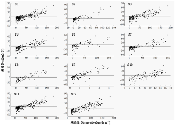
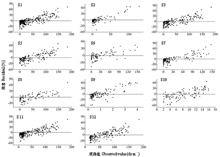
与观测值相比,RF和SGT的预测值都存在低值区高估和高值区低估的现象,导致残差出现线性趋势（图8和图9）。上述现象出现在各情景中。被高估的值出现于有人类管理活动的绿洲内部地区（用低含盐水灌溉）,而被低估的值分布于绿洲的外围（盐分来自于上游灌区）,即灌溉区盐分在绿洲-荒漠交错带的聚集区,以及渭库绿洲的东北角。

图8

新窗口打开|下载原图ZIP|生成PPT
图8不同情景下基于RF预测的残差与观测值的对比

Fig. 8Scatterplot of the residuals predicted by RF versus the measured soil salinity in each scenario

图9

新窗口打开|下载原图ZIP|生成PPT
图9不同情景下基于SGT预测的残差与观测值的对比

Fig. 9Scatterplot of the residuals predicted by SGT versus the measured soil salinity in each scenario

2.3 情景分区建模的预测精度

表3和表4显示了1.2.7 节中方案一获得的统计结果：（1）对于RF来说, 以下6个情景IS模式（表 3） 的预测精确高于RS模式（表 4）：情景2,5,6,9,10,12。以 RPD 值为例,上述方案的精度分别提升了4.23%、3.23%、2.21%、1900%、620% 和11.11%。其余4个情景的RS模式（表3）的预测精确高于IS模式：情景3、11、7、8。RPD 值增加了3.14%、2.4%、13.97% 和2.38%。（2）对于SGT来说,以下6个情景IS模式（表3）的预测精确高于RS模式（表4）：情景5、6、8、9、10、12。RPD 值分别增加了4.84%、8.22%、2180%、540%、12.73% 和12.00%。反之,RS模式（表3）的预测精确高于IS模式的情景为：情景2、3、7。RPD 值增加5.97%、2.38% 和2.11%。

表5显示了2.2.7 节中方案二中的统计结果 （图 5）。首先,将情景9和11的预测值合并,CS与RSOSM模式结果对比：基于SGT,R² 和 RPD 分别提升了14.59% 和6.47%,基于RF,分别提升了10.87% 和4.38%。其次,当情景2和3的预测值合并后,CS与RSOSM模式结果相比：基于SGT,R² 和 RPD 分别降低了2.17%和2.90%,基于RF,二者分别降低了2.08%和1.46%。地貌分组当中的情景7和8合并后,CS与RSOSM模式结果相比：SGT的预测结果显示,前者模式中R² 值上升了8.51%,RPD下降了3.62%,RF预测结果显示,R²下降了 7.00%,RPD 值下降了3.03%。当草地和未用土地的预测值组合时,CS与RSOSM模式结果对比,对于SGT,前者相比后者,预测精度增加17.50%（R²）和5.38%（RPD）,基于RF,预测精度提高了7.50%（R²）和2.32%（RPD）。

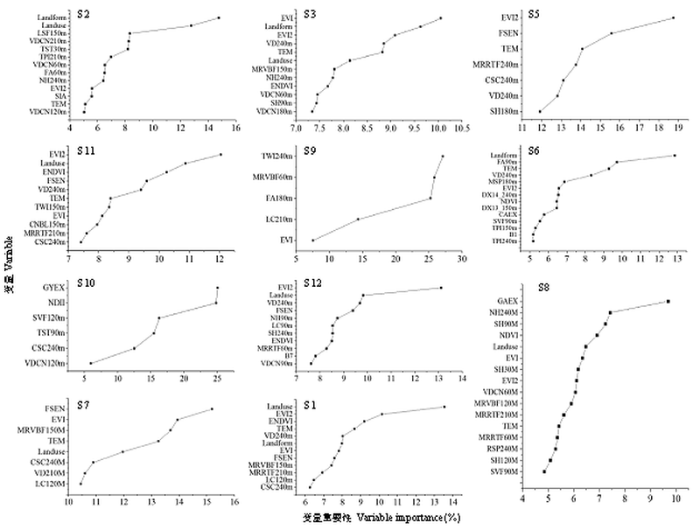
2.4 不同情景分区指示土壤盐度变化的重要变量

图10显示了10个情景模式下各自最优变量集。RF和SGT都可产生变量的贡献度,这里只显示精度相对较高的算法获取的变量及其贡献度。将变量的贡献度进行归一化处理后经对比发现,由于外部环境或者所处地理位置的影响,各情景的关键变量组有一定的差异性。同时,研究根据变量计算的数据来源,重新核算了影响盐渍化空间差异性的贡献度。结果显示,基于地形衍生的变量组（多空间分辨率）的贡献度最高,平均值为52.98%,其次为Landsat衍生变量组,平均值为36.22%,地貌类型的平均贡献度为11.29%,土地利用的平均贡献度为10.51%。对比所有情景发现,仅从变量出现的频次考虑,地表温度,EVI2,EVI,ENDVI,FSEN依次出现了7次、6次、6次、4次、4次。另外,地貌和土地利用在下列情景中的贡献度位居前列：情景1、2、3、11、12。

图10

新窗口打开|下载原图ZIP|生成PPT
图10不同情景下基于1.2.6节中介绍的方法迭代获取的重要变量

Fig. 10Important variables iteratively obtained based on the methods described in Section 1.2.6 in different scenarios

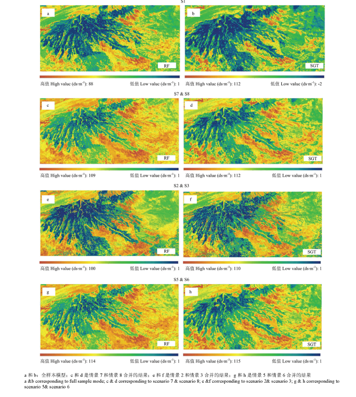
2.5 土壤盐度的空间分布特征

根据第1.2.6节的方法,获取RF和SGT两种算法迭代产生的模型,并绘制了研究区土壤盐渍化的空间分布图（图11）。图11中的a和b图显示了全样本模型的预测结果,c和d,e和f,g和h分别对应情景7和8,情景3和2,情景5和6。地貌的2个类型与土地利用中2个类型各自合并后,并不能覆盖全绿洲,合并后外围的数据则由全样本模型的预测值进行填充。整体而言,从定性层面来看,上述结果与DING等^[23]与WANG等^[25]结果相近。绿洲内部,灌区农业种植区的土壤盐度相对较低,由于地形地势的引导,盐分都积聚在绿洲-荒漠过渡带地区。

图11

新窗口打开|下载原图ZIP|生成PPT
图11基于RF和SGT预测的研究区土壤盐度空间分布特征。

Fig. 11Spatial distribution of soil salinity (dS·m^-1) predicted by SGT and RF for three combined modes and the full sample model (Table 5) in the study area

3 讨论

3.1 RF和SGT的精度评价

观察表3、4和5后发现,27个情景中的18个（接近70%）都显示 SGT的预测精度高于RF。此结果暗示,SGT相对更适合预测干旱区土壤盐度空间变异性。然而,上述两种算法在盐渍化研究中并无比较的先例,在此仅引用其他研究加以说明。NAGHIBI等基于SGT,CART和RF研究阿富汗地区地下水喷泉潜在分布区,结果显示,SGT的预测效果最佳,其次为CART和RF^[38]。YOUSSEF等^[39]基于广义线性模型（Generalized Linear Models,GLM),CART,SGT和RF评价沙特阿拉伯地区滑坡灾害危险性,AUC（Area Under the Curve ) 曲线结果显示,SGT的值最高,为0.958,其次为GLM,为0.821,CART为0.816,最后为RF,0.783。值越大代表精度越高。YANG等^[40]比较SGT与RF预测青藏高原东北部高植被覆盖区土壤有机质的空间分布,结果显示,SGT的预测精度稍高于RF,二者预测的结果在空间分布上较为相似。

基于上述两种算法的模拟值出现低值高估和高值低估的现象已出现在其他研究中^[41,42]。主要的原因在于小数据集样本的代表性不足。本研究的样本设计起初是以绿洲尺度为前提而定,并不是完全基于小尺度而定。聚焦至不同情景下,样点的代表性可能有所下降,致使该模式（全样本建模）下并不是每个情景的预测精度都可以达到绿洲尺度的水平。上述现象可能无法完全避免,在于研究区土壤盐度空间变异性较强。样本的设计依据来自于环境变量,这些变量在空间分布上并不能完全与土壤属性呈高度一致性变化。对此,面对复杂的变异环境需要加入更多不同类型且更为普及的高空间分辨率传感器进行相互校正或能提高样本的代表性,以及满足大尺度制图的需求。

基于Landsat 数据建立土壤盐度模型的案例已有报道（表1）。涉及的深度包括0—10、0—20和0—30 cm,部分研究未列出深度。参与建模的样本量残次不齐。选择的变量或为单一变量或为变量组。相关性有高有低（R² = 0.874,R² = 0.564,R² = 0.483,R² = 0.78,R² = 0.45,R² = 0.71,R² = 0.93,等）。选择的方法各有优缺点（线性、多元线性方程、神经网络、支持向量机、指数模型等）。验证模型包括设定训练样本/验证样本的比例和十字交叉验证。同时,各自的地理环境也有明显的差异性。由于上述多维信息的差异性,不能直接对比。但本研究认为所得结果进一步丰富了该领域关于环境-土壤盐渍化关系知识库。

3.2 情景分区建模对绿洲土壤盐度预测精度的影响

表3和表4中情景2、5、6、8、9、10、12,共计7个情景（占70%）的结果显示了分区建模的有效性。其中EC≤4 dS·m^-1和2 dS·m^-1＜EC＜16 dS·m^-1两个情景的IS模式精度显著高于RS模式。原因可能归结于用于绿洲尺度建模的盐度变异性与上述范围的变异性相差太大,二者数据的值域范围重叠度较低。此外,低盐度区域如农田,其土壤中盐度的空间变异性与外界环境的变化同步性较其他地区并不明显,控制该区植被生长的关键变量以土壤水分为主。同时,用于测试低盐度的仪器在该区的测试精度并不稳定。因此上述结果给我们的启示在于绿洲尺度的模型并不适用于灌溉区,需要在此情景下单独建立相应的预测模型。

表5中的组合场景再次验证了样本数据分割（根据地理特征）对提高土壤盐度预测精度的重要性。场景9和场景11组合可以有效地提高预测精度,这是所有4种组合中精度提高最明显的。对表5结果的综合比较表明,当有历史土壤电导率数据时,它们是首选子区分割参考媒介。RF结果显示了场景2和3被组合在一起时提高了预测精度。这表明植被覆盖对土壤盐度预测有一定的影响。然而,由于植被类型多样,精度的提高范围有限,因为一定程度的概率表明,同为植被覆盖下有着相似NDVI值的单一或多种植被类型有着不同的土壤电导率值。利用地貌单元作为相对均匀区域的划分基础结果表明可以有效提高预测精度。这些结果的优势是分区范围相对稳定,极少随时间变化。这与与母质有关,后者与土壤盐渍化的发生和发展有间接关系^[4,43]。土地利用数据的重要性（它整合了人类活动信息用以提高土壤盐度预测的准确性）排在情景9和11（参考R²和RPD）的组合之后。这一发现也反映在各场景的重要变量排序中。值得注意的是,上述的基于地形和土地利用分区子区域,只覆盖了整个绿洲的两种类型,在下最终结论之前,我们还需要收集一定数量的样本进一步验证。

3.3 不确定性分析

全面分析上述结果后,未来的研究可能需要考虑以下几个方面：（1）绿洲尺度下采样点设计不仅要考虑整个研究区,还要考虑子区域,并将道路可达性和采样成本考虑在内。虽然该研究在每个子区测试了模拟结果,预测误差降低,如果在该区中收集更多代表性样本,预测的准确性将得到显著改善。（2）由于混合像元问题,现存遥感或数字档案数据与地理现象无法实现精确匹配。这个过程需要使用更高的空间分辨率数据。（3）在一定土壤盐度值范围内,植被物种多样性和土壤的复杂性加剧了不确定性。（4）当土壤中的盐含量低于15%时,响应变化不能从外界观察得到,这就增加了两种情况下的探查难度：一种是在农业作物区,另一种是深层地下水已经停止积盐。（5）遥感数据,即使经过了大气校正和地形校正,在后续流程仍有一定的错误积累。

4 结论

在本研究中模拟的27个场景中（12个原始和15个衍生）,70.37%的情景证明SGT比RF有更高的预测精度。因此,相对而言,在干旱区SGT比RF更适合于预测复杂环境下土壤盐度的空间变异性。

将绿洲划分为若干子区,然后结合子区的预测值,能有效地提高绿洲尺度的预测精度。此结论特别适用于EC≤4 dS·m^-1和2 dS·m^-1＜EC＜16 dS·m^-1两个情景,需要单独预测。首选分区媒介是土壤电导率（前提是数据能够反映当前土壤盐度变异性）,其次是地形和土地利用。

通过对多个情景优化数据集的比较,以下变量对于指示子区或绿洲尺度的土壤盐度预测具有重要的作用：土地利用、地貌、EVI、EVI2、FSEN、TEM、ENDVI以及多种空间分辨率的地形变量。

研究建议为了达到全组分景观单元都保持较高的属性预测精度,应该在样本设计上着手,并经过反复测试找到最为合适的景观分区变量,分区媒介的选择可以从驱动或者响应变量入手。

参考文献 View Option 原文顺序
文献年度倒序
文中引用次数倒序
被引期刊影响因子

[1] ALLBED A, KUMAR L, ALDAKHEEL Y Y . Assessing soil salinity using soil salinity and vegetation indices derived from IKONOS high-spatial resolution imageries: Applications in a date palm dominated region
Geoderma, 2014,230:1-8.
DOI:10.1016/j.geoderma.2014.03.025URL [本文引用: 7]
61Assessing soil salinity in a date palm dominated region using vegetation and soil salinity indices, extracted from IKONOS satellite images.61The SAVI, NDSI and SI-T indices were the most useful indices.61The NDSI and SI-T indices works well in areas with low vegetation cover to assess soil salinity.61The SAVI index, yield better results for assessing soil salinity in densely vegetated areas.

[2] SCUDIERO E, SKAGGS T H, CORWIN D L . Regional scale soil salinity evaluation using Landsat 7, western San Joaquin Valley, California, USA.
Geoderma Regional, 2014(2/3):82-90.
DOI:10.1016/j.geodrs.2014.10.004URL [本文引用: 1]
61Relationships between soil salinity and Landsat 7 crop reflectance were studied.61Multi-year analysis of Landsat 7 data highlights soil salinity effects.61Between fields, the Landsat 7–salinity relationships vary according to soil type.61Between years, the relationships vary according to meteorological conditions.

[3] SCUDIERO E, SKAGGS T H, CORWIN D L . Regional-scale soil salinity assessment using Landsat ETM + canopy reflectance
Remote Sensing of Environment, 2015,169:335-343.
DOI:10.1016/j.rse.2015.08.026URL [本文引用: 3]
61Multi-year maxima of Landsat ETM+ vegetation indices correlates with soil salinity.61Linear regressions provide reliable salinity estimates at the regional scale.61Crop and meteorological covariates increase accuracy of soil salinity predictions.61Salinity assessment models are validated through a spatial cross-validation.

[4] TAGHIZADEH-MEHRJARDI R, MINASNY B, SARMADIAN F, MALONE B P . Digital mapping of soil salinity in Ardakan region, central Iran
Geoderma, 2014,213:15-28.
DOI:10.1016/j.geoderma.2013.07.020URL [本文引用: 7]
Salinization and alkalinization are the most important land degradation processes in central Iran. In this study we modelled the vertical and lateral variation of soil salinity (measured as electrical conductivity in saturation paste, ECe) using a combination of regression tree analysis and equal-area smoothing splines in a 72,000ha area located in central Iran. Using the conditioned Latin hypercube sampling method, 173 soil profiles were sampled from the study area, and then analysed for ECe and other soil properties. Auxiliary data used in this study to represent predictive soil forming factors were terrain attributes (derived from a digital elevation model), Landsat 7 ETM+ data, apparent electrical conductivity (ECa)—measured using an electromagnetic induction instrument (EMI), and a geomorphologic surfaces map. To derive the relationships between ECe (from soil surface to 1m) and the auxiliary data, regression tree analysis was applied. In general, results showed that the ECa surfaces are the most powerful predictors for ECe at three depth intervals (i.e. 0–15, 15–30 and 30–60cm). In the 60–100cm depth interval, topographic wetness index was the most important parameter used in regression tree model. Validation of the predictive models at each depth interval resulted in R2 values ranging from 78% (0–15cm) to 11% (60–100cm). Thus we can recommend similar applications of this technique could be used for mapping soil salinity in other parts in Iran.

[5] WU W, MHAIMEED A S , AL-SHAFIE W M,ZIADAT F,DHEHIBI B,NANGIA V,PAUW E D.Mapping soil salinity changes using remote sensing in Central Iraq
Geoderma Regional, 2014(2/3):21-31.
DOI:10.1016/j.geodrs.2014.09.002URL [本文引用: 3]
61A multiyear maxima-based modeling approach was proposed for salinity mapping.61Vegetated and non-vegetated areas were separately treated.61Developed salinity models can reliably predict soil salinity (82.56%).61Multitemporal salinity maps reveal strong salinity change in space and time.61Salinity dynamics is mainly related to land use and management of farmers.

[6] YAHIAOUI I, DOUAOUI A, QIANG Z, ZIANE A . Soil salinity prediction in the Lower Cheliff plain(Algeria) based on remote sensing and topographic feature analysis
Journal of Arid Land, 2015,7(6):794-805.
DOI:10.1007/s40333-015-0053-9URL [本文引用: 1]
Soil salinity and ground surface morphology in the Lower Cheliff plain (Algeria) can directly or indirectly impact the stability of environments. Soil salinization in this area is a major pedological problem related to several natural factors, and the topography appears to be important in understanding the spatial distribution of soil salinity. In this study, we analyzed the relationship between topographic parameters and soil salinity, giving their role in understanding and estimating the spatial distribution of soil salinity in the Lower Cheliff plain. Two satellite images of Landsat 7 in winter and summer 2013 with reflectance values and the digital elevation model (DEM) were used. We derived the elevation and slope gradient values from the DEM corresponding to the sampling points in the field. We also calculated the vegetation and soil indices (i.e. NDVI (normalized dif-ference vegetation index), RVI (ratio vegetation index), BI (brightness index) and CI (color index)) and soil salinity indices, and analyzed the correlations of soil salinity with topography parameters and the vegetation and soil indices. The results showed that soil salinity had no correlation with slope gradient, while it was sig-nificantly correlated with elevation when the EC (electrical conductivity) values were less than 8 dS/m. Also, a good relationship between the spectral bands and measured soil EC was found, leading us to define a new salinity index, i.e. soil adjusted salinity index (SASI). SASI showed a significant correlation with elevation and measured soil EC values. Finally, we developed a multiple linear regression for soil salinity prediction based on elevation and SASI. With the prediction power of 45%, this model is the first one developed for the study area for soil salinity prediction by the combination of remote sensing and topographic feature analysis.

[7] ZHANG T T, QI J G, GAO Y, OUYANG Z T, ZENG S L, ZHAO B . Detecting soil salinity with MODIS time series VI data
Ecological Indicators, 2015,52:480-489.
DOI:10.1016/j.ecolind.2015.01.004URL [本文引用: 1]
Mapping of salinization using the satellite derived vegetation indices (VIs) remains difficult at broad regional scales due to the low classification accuracy. Satellite derived VIs from the Moderate Resolution Imaging Spectroradiometer (MODIS) have more potential because the MODIS balances the requirements of spatial detail, spectral and temporal density and tends to reflect vegetation responses through time. However, the relationship between MODIS data and salinity may be underestimated in previous studies because the MODIS time series data were not investigated thoroughly, especially regarding vegetation phenology. This study assessed the applicability of MODIS time series VI data for monitoring soil salinization with a series of MODIS pixels selected in the Yellow River Delta, China. The hidden information in vegetation phenology was investigated by improving the quality of VIs time series data with the Savitzky olay filter, extracting the phenological markers and differentiating VIs time series data based on vegetation types. The results showed that the quality of the enhanced vegetation index (EVI) time series data were improved by the Savitzky olay filter, which could provide more accurate thresholds of phenological stages than the empirical definition. The seasonal integral of EVI (EVI-SI) extracted from the smoothed EVI time series profile was verified as the best indicator of the degree of soil salinity. Additionally, the correlation of EVI-SI and soil salinity was highly dependent on land cover heterogeneity, and the ranges of correlation coefficients were as high as 0.59 0.92. EVI-SI was linearly correlated with ECe in cropland with a high model fit (R2=0.85). The relationship of EVI-SI and ECe fit best with a binomial line and EVI-SI was able to explain 70% of the variance of ECe. Despite the poor fit of the linear regression model in mixed sites limited by spatial resolution (R2=0.32), MODIS time series VI data, as well as the extracted seasonal parameters, still show great potential to assess large-scale soil salinization.

[8] ZHANG T-T, ZENG S-L, GAO Y, OUYANG Z-T, LI B, FANG C-M, ZHAO B . Using hyperspectral vegetation indices as a proxy to monitor soil salinity
Ecological Indicators, 2011,11(6):1552-1562.
DOI:10.1016/j.ecolind.2011.03.025URL [本文引用: 1]
The spectral bands most sensitive to salt-stress across diverse plants have not yet been defined; therefore, the predictive ability of previous vegetation indices (VIs) may not be satisfied for salinization monitoring. The hyperspectra of seven typical salt-sensitive/halophyte species and their root-zone soil samples were collected to investigate the relationship between vegetation spectra and soil salinity in the Yellow River Delta (YRD) of China. Several VIs were derived from the recorded hyperspectra and their predictive power for salinity was examined. Next, a univariate linear correlogram as well as multivariate partial least square (PLS) regression was employed to investigate the sensitive bands. VIs examination and band investigation confirmed that the responses of the vegetation differed from species to species, which explained the vibrations of the VIs in many study cases. These differences were primarily between salt-sensitive and halophyte plants, with the former consistently having higher sensitivity than the latter. With the exception of soil adjusted vegetation index (SAVI), most VIs were found to have weak relationships with soil salinity (with average of 0.28) and some were not sensitive to all species [ and four SASIs for all species, with largely improved values ranging from 0.50 to 0.58. Our findings indicate the potential to monitor soil salinity with the hyperspectra of salt-sensitive and halophyte plants.

[9] GARCíA M, OYONARTE C, VILLAGARCíA L, CONTRERAS S, DOMINGO F, PUIGDEFáBREGAS J . Monitoring land degradation risk using ASTER data: The non-evaporative fraction as an indicator of ecosystem function
Remote Sensing of Environment, 2008,112(9):3720-3736.
DOI:10.1016/j.rse.2008.05.011URL [本文引用: 1]
There is a need to develop operational land degradation indicators for large regions to prevent losses of biological and economic productivity. Disturbance events press ecosystems beyond resilience and modify the associated hydrological and surface energy balance. Therefore, new indicators for water-limited ecosystems can be based on the partition of the surface energy into latent (E) and sensible heat flux (H). In this study, a new methodology for monitoring land degradation risk for regional scale application is evaluated in a semiarid area of SE Spain. Input data include ASTER surface temperature and reflectance products, and other ancillary data. The methodology employs two land degradation indicators, one related to ecosystem water use derived from the non-evaporative fraction (NEF = H / ( E + H)), and another related to vegetation greenness derived from the NDVI. The surface energy modeling approach used to estimate the NEF showed errors within the range of similar studies ( R 2 = 0.88; RMSE = 0.18 (22%)). To create quantitative indicators suitable for regional analysis, the NEF and NDVI were standardized between two possible extremes of ecosystem status: extremely disturbed and undisturbed in each climatic region to define the NEFS (NEF Standardized) and NDVIS (NDVI Standardized). The procedure was successful, as it statistically identified ecosystem status extremes for both indicators without supervision. Evaluation of the indicators at disturbed and undisturbed (control) sites, and intermediate surface variables such as albedo or surface temperature, provided insights on the main surface energy status controls following disturbance events. These results suggest that ecosystem functional indicators, such as the NEFS, can provide information related to the surface water deficit, including the role of soil properties.

[10] LI X, YANG K, ZHOU Y. Progress in the study of oasis-desert interactions.
Agricultural and Forest Meteorology 2016,230-231:1-7. DOI: 10.1016/j.agrformet.2016.08.022
DOI:10.1016/j.agrformet.2016.08.022URL [本文引用: 3]
Within arid and semi-arid regions, deserts and oases generally act as the landscape matrix and mosaic, respectively. Oasis-desert interactions, i.e., the transport of mass and energy between the two, are very important for the stable co-existence of oasis and desert ecosystems. In recent decades, great progress has been made to advance our understanding of oasis-desert interactions. In this preface, we provide an overview of oasis-desert interaction studies available in the literature and our current understanding of the limitations and challenges of these studies. Future foci can be multiple-scale, high-accuracy observing matrices and seamless simulations from mesoscale circulations to large eddies, which are crucial for understanding small-scale structures of energy and water exchange and their connection with oasis-desert interaction.

[11] GONG L, RAN Q, HE G, TIYIP T . A soil quality assessment under different land use types in Keriya river basin, Southern Xinjiang, China
Soil and Tillage Research, 2015,146:223-229.
DOI:10.1016/j.still.2014.11.001URL [本文引用: 1]
The process of oasisization leads to the transformation of natural land use to farmlands in the Keriya river basin. In order to investigate changes in soil quality during the process of oasisization, we established five experimental fields in the oasis-desert ecotone of the Keriya river basin, including farmlands(FL) and four typical natural lands natural forest (NF), saline and alkaline land (SAL), desert (D) and sand land (SL)) of the main local land cover. In this paper, a minimum data set of soil indicators was selected including soil water content indicator, pH, soil nutrient indicators and soil salinity indicators, with 100 soil samples collected within five land use types. Observations found significant differences in the fifteen soil indicators. These were used to calculate a soil quality index (SQI) and assessed using multivariate analyses (cluster analysis and principal component analysis, PCA) in order to determine the soil quality of the different land uses. Data indicated a clear difference in soil quality among the studied areas: low soil quality (SQI<0.55) in SAL, D and SL; intermediate soil quality (0.55<SQI<0.70) in FL and NF. Results suggested that the soil of the oasis-desert ecosystem has low soil water content, high concentrations of salt and a structureless soil with very low organic matter, but concentrations of soil nutrients increased and land improvement occurred after land use shifts from natural land uses to cultivation. The four natural lands have distinct soil characteristics, which should be considered during the process of soil reclamation.

[12] TUTEJA N K, BEALE G, DAWES W, VAZE J . Predicting the effects of landuse change on water and salt balance-a case study of a catchment affected by dryland salinity in NSW, Australia
Journal of Hydrology, 2003,283(1):67-90.
DOI:10.1016/S0022-1694(03)00236-1URL [本文引用: 1]
An integrated and comprehensive framework for the assessment of water and salt balance for large catchments is presented. The framework is applied to the Mandagery Creek catchment (1688 km 2), located in the south-eastern part of Australia. The catchment is affected by dryland salinity and the effects of landuse, climate, topography, soils and geology on water and salt balance are examined. Landuse change scenarios designed to: (a) increase the perennial content of the pastures and crop rotations and (b) increase the current remnant native woody vegetation with additional tree cover are investigated to determine the level of intervention required to develop ameliorative strategies. Likely downstream impacts of the reduction in water flow and salt export are also estimated.

[13] WANG Y, LI Y . Land exploitation resulting in soil salinization in a desert-oasis ecotone
Catena, 2013,100:50-56.
DOI:10.1016/j.catena.2012.08.005URL [本文引用: 1]
78 Land exploitation strongly influenced soil properties. 78 38% of the studied area experienced transitional land-use changes. 78 Soil salt accumulation per unit area increased by 60%. 78 Salt accumulation resulted from increased irrigation as more land transitioned to farmland. 78 A lesson to be learned the hard way for similar ecotones in arid zones.

[14] HENGL T , MENDES D J J, HEUVELINK G B, RUIPEREZ G M, KILIBARDA M, BLAGOTI? A, SHANGGUAN W, WRIGHT M N, GENG X, BAUERMARSCHALLINGER B. SoilGrids250m: Global gridded soil information based on machine learning
Plos One, 2017,12(2):e0169748.
DOI:10.1371/journal.pone.0169748URLPMID:5313206 [本文引用: 1]
This paper describes the technical development and accuracy assessment of the most recent and improved version of the SoilGrids system at 250m resolution (June 2016 update). SoilGrids provides global predictions for standard numeric soil properties (organic carbon, bulk density, Cation Exchange Capacity (CEC), pH, soil texture fractions and coarse fragments) at seven standard depths (0, 5, 15, 30, 60, 100 and 200 cm), in addition to predictions of depth to bedrock and distribution of soil classes based on the World Reference Base (WRB) and USDA classification systems (ca. 280 raster layers in total). Predictions were based on ca. 150,000 soil profiles used for training and a stack of 158 remote sensing-based soil covariates (primarily derived from MODIS land products, SRTM DEM derivatives, climatic images and global landform and lithology maps), which were used to fit an ensemble of machine learning methods andom forest and gradient boosting and/or multinomial logistic regression s implemented in theRpackagesranger,xgboost,nnetandcaret. The results of 10 old cross-validation show that the ensemble models explain between 56% (coarse fragments) and 83% (pH) of variation with an overall average of 61%. Improvements in the relative accuracy considering the amount of variation explained, in comparison to the previous version of SoilGrids at 1 km spatial resolution, range from 60 to 230%. Improvements can be attributed to: (1) the use of machine learning instead of linear regression, (2) to considerable investments in preparing finer resolution covariate layers and (3) to insertion of additional soil profiles. Further development of SoilGrids could include refinement of methods to incorporate input uncertainties and derivation of posterior probability distributions (per pixel), and further automation of spatial modeling so that soil maps can be generated for potentially hundreds of soil variables. Another area of future research is the development of methods for multiscale merging of SoilGrids predictions with local and/or national gridded soil products (e.g. up to 50 m spatial resolution) so that increasingly more accurate, complete and consistent global soil information can be produced. SoilGrids are available under the Open Data Base License.

[15] SCHILLACI C, LOMBARDO L, SAIA S, FANTAPPIè M ,M?RKER M,ACUTIS M. Modelling the topsoil carbon stock of agricultural lands with the Stochastic Gradient Treeboost in a semi-arid Mediterranean region
Geoderma, 2017,286:35-45.
DOI:10.1016/j.geoderma.2016.10.019URL [本文引用: 1]
61Soil organic carbon (SOC) stock was estimated in a Mediterranean area using digital soil mapping techniques.61Climate, texture and land use were found to be important predictors.61The model used greatly improved SOC stock estimation compared to previous estimates.61The panchromatic band of Landsat ETM+ 7 was more predictive compared to NDVI.

[16] HASTIE T, TIBSHIRANI R, FRIEDMAN J H, FRANKLIN J . The elements of statistical learning, second edition: data mining, inference, and prediction
Mathematical Intelligencer, 2009,27(2):83-85.
[本文引用: 1]

[17] ANGILERI S E, CONOSCENTI C, HOCHSCHILD V ,M?RKER M, ROTIGLIANO E, AGNESI V. Water erosion susceptibility mapping by applying Stochastic Gradient Treeboost to the Imera Meridionale River Basin (Sicily, Italy)
Geomorphology, 2016,262:61-76.
DOI:10.1016/j.geomorph.2016.03.018URL [本文引用: 3]
61We explore the ability of Stochastic Gradient Treeboost in predicting the spatial occurrence of soil erosion processes.61The overall accuracy of the susceptibility models is excellent.61The relationships between erosion processes and predictors is analyzed.61We design a methodological approach to create combined erosion susceptibility maps.

[18] HEUNG B, BULMER C E, SCHMIDT M G . Predictive soil parent material mapping at a regional-scale: A Random Forest approach
Geoderma, 2014,214:141-154.
DOI:10.1016/j.geoderma.2013.09.016URL [本文引用: 2]
61Soil parent material was mapped over a large spatial extent.61Topographic indices and soil survey data were used to predict parent material.61Optimization of mtry and variable reduction was examined.61Predictive parent material mapping was assessed using soil survey and point data.

[19] HEUNG B, HO H C, ZHANG J, KNUDBY A, BULMER C E, SCHMIDT M G . An overview and comparison of machine-learning techniques for classification purposes in digital soil mapping
Geoderma, 2016,265:62-77.
DOI:10.1016/j.geoderma.2015.11.014URL [本文引用: 1]
61Soil taxonomic units were mapped for the Lower Fraser Valley.6110 machine-learning algorithms were compared.61Four methods of developing training data were compared.61Sampling from soil surveys using an area-weighted approach was most effective.61Choice of model and sampling design greatly influences outputs.

[20] LIE? M, GLASER B, HUWE B . Uncertainty in the spatial prediction of soil texture: Comparison of regression tree and Random Forest models
Geoderma, 2012,170:70-79.
DOI:10.1016/j.geoderma.2011.10.010URL [本文引用: 1]
78 Soil texture is predicted on a landscape scale. 78 Regression Trees and Random Forest models are compared in their performance. 78 The digital soil maps include model variability and prediction uncertainty. 78 Model dependence on the dataset is addressed by model runs with various data subsets. 78 Surface processes are distinguished from the influence of parent material.

[21] BREIMAN L. . Random Forests Machine Learning, 2001,45(1):5-32.
[本文引用: 2]

[22] FRIEDMAN J H. Stochastic Gradient Boosting
Computational Statistics & Data Analysis, 2002,38(4):367-378.
[本文引用: 1]

[23] DING J, YU D. Monitoring and evaluating spatial variability of soil salinity in dry and wet seasons in the Werigan-Kuqa Oasis,China,using remote sensing and electromagnetic induction instruments.
Geoderma ,2014,235 236:316-322.
DOI:10.1016/j.geoderma.2014.07.028URL [本文引用: 2]
61Data from remote and near sensing sources are combined to study soil salinity.61Soil samples from field work are used for verification.61Commonly employed spatial interpolation approaches predict soil salinity in space.

[24] BENNETT S J, BARRETTLENNARD E G, COLMER T D . Salinity and waterlogging as constraints to saltland pasture production: a review
Agriculture Ecosystems & Environment, 2009,129(4):349-360.
DOI:10.1016/j.agee.2008.10.013URL [本文引用: 1]
This review considers the issue of targeting plants for forage/fodder production in landscapes affected by dryland salinity, and two principal factors that affect saltland capability alinity and waterlogging. Saltland differs in its capacity to support plant growth, and the species used differ in grazing value, so that greatest economic gain will be achieved by focusing revegetation into areas of highest capability. Both salinity and waterlogging are temporally and spatially variable: plant ecological zonation on saltland is a reflection of plant adaptation to these variable stresses. The review has three parts. First, we consider the case for ecological zonation to be caused by variation in salinity and waterlogging. Secondly, we review the current means by which salinity and waterlogging are measured and the suitability of these techniques for rapid field appraisal of saltland capability. Thirdly, we suggest three critical questions that need to be answered if we are to establish a framework to make rapid saltland capability assessments. These are: (a) can a plant use the groundwater, (b) is the soil water above the water table suitable for use, and for what period is it sufficient in volume to support growth, and (c) is the soil sufficiently aerobic for root-growth and function. We conclude with some recommendations about the types of data around which a saltland capability assessment protocol might be designed.

[25] WANG F, CHEN X, LUO G, HAN Q . Mapping of regional soil salinities in Xinjiang and strategies for amelioration and management
Chinese Geographical Science, 2015,25(3):321-336.
DOI:10.1007/s11769-014-0718-xURL [本文引用: 2]
Abstract: Information on the spatial distribution of soil salinity can be used as guidance in avoiding the continued degradation of land and water resources by better informing policy makers. However, most regional soil-salinity maps are produced through a conventional direct-linking method derived from historic observations. Such maps lack spatial details and are limited in describing the evolution of soil salinization in particular instances. To overcome these limitations, we employed a method that included an integrative hierarchical-sampling strategy (IHSS) and the Soil Land Inference Model (SoLIM) to map soil salinity over a regional area. A fuzzy c-means (FCM) classifier is performed to generate three measures, comprising representative grade, representative area, and representative level (membership). IHSS employs these three measures to ascertain how many representative samples are appropriate. Through this synergetic assessment, representative samples are obtained and their soil-salinity values are measured. These samples are input to SoLIM, which is constructed based on fuzzy logic, to calculate the soil-forming environmental similarities between representative samples and other locations. Finally, a detailed soil-salinity map is produced through an averaging function that is linearly weighted, which is used to integrate the soil salinity value and soil similarity. This case study, in the Uyghur Autonomous Region of Xinjiang of China, demonstrates that the employed method can produce soil salinity map at a higher level of spatial detail and accuracy. Twenty-three representative points are determined. The results show that 1) the prediction is appropriate in Kuqa Oasis ( R 2 = 0.70, RPD = 1.55, RMSE = 12.86) and Keriya Oasis ( R 2 = 0.75, RPD = 1.66, RMSE = 10.92), that in Fubei Oasis ( R 2 = 0.77, RPD = 2.01, RMSE = 6.32) perform little better than in those two oases, according to the evaluation criterion. 2) Based on all validation samples from three oases, accuracy estimation show the employed method ( R 2 = 0.74, RPD = 1.67, RMSE = 11.18) performed better than the multiple linear regression model ( R 2 = 0.60, RPD = 1.47, RMSE = 14.45). 3) The statistical result show that approximately half (48.07%) of the study area has changed to salt-affected soil, mainly distributed in downstream of oases, around lakes, on both sides of rivers and more serious in the southern than the northern Xinjiang. To deal with this issue, a couple of strategies involving soil-salinity monitoring, water management, and plant diversification are proposed, to reduce soil salinization. Finally, this study concludes that the employed method can serve as an alternative model for soil-salinity mapping on a large scale.

[26] MINASNY B, MCBRATNEY A B . A conditioned Latin hypercube method for sampling in the presence of ancillary information
Computers & Geosciences, 2006,32(9):1378-1388.
DOI:10.1016/j.cageo.2005.12.009URL [本文引用: 1]
This paper presents the conditioned Latin hypercube as a sampling strategy of an area with prior information represented as exhaustive ancillary data. Latin hypercube sampling (LHS) is a stratified random procedure that provides an efficient way of sampling variables from their multivariate distributions. It provides a full coverage of the range of each variable by maximally stratifying the marginal distribution. For conditioned Latin hypercube sampling (cLHS) the problem is: given N sites with ancillary variables ( X), select x a sub-sample of size n ( n N ) in order that x forms a Latin hypercube, or the multivariate distribution of X is maximally stratified. This paper presents the cLHS method with a search algorithm based on heuristic rules combined with an annealing schedule. The method is illustrated with a simple 3-D example and an application in digital soil mapping of part of the Hunter Valley of New South Wales, Australia. Comparison is made with other methods: random sampling, and equal spatial strata. The results show that the cLHS is the most effective way to replicate the distribution of the variables.

[27] 鲁如坤 . 土壤农业化学分析方法.北京: 中国农业科技出版社, 1999.
[本文引用: 1]

LU R K. Methods for Soil Agrochemistry Analysis. Beijing: China Agricultural Science and Technology Press, 1999. (in Chinese).
[本文引用: 1]

[28] SONG W, MU X, RUAN G, GAO Z, LI L, YAN G . Estimating fractional vegetation cover and the vegetation index of bare soil and highly dense vegetation with a physically based method
International Journal of Applied Earth Observations & Geoinformation, 2017,58:168-176.
DOI:10.1016/j.jag.2017.01.015URL [本文引用: 1]
Normalized difference vegetation index (NDVI) of highly dense vegetation (NDVIv) and bare soil (NDVIs), identified as the key parameters for Fractional Vegetation Cover (FVC) estimation, are usually obtained with empirical statistical methods However, it is often difficult to obtain reasonable values of NDVIvand NDVIsat a coarse resolution (e.g., 1km), or in arid, semiarid, and evergreen areas. The uncertainty of estimated NDVIsand NDVIvcan cause substantial errors in FVC estimations when a simple linear mixture model is used. To address this problem, this paper proposes a physically based method. The leaf area index (LAI) and directional NDVI are introduced in a gap fraction model and a linear mixture model for FVC estimation to calculate NDVIvand NDVIs. The model incorporates the Moderate Resolution Imaging Spectroradiometer (MODIS) Bidirectional Reflectance Distribution Function (BRDF) model parameters product (MCD43B1) and LAI product, which are convenient to acquire. Two types of evaluation experiments are designed 1) with data simulated by a canopy radiative transfer model and 2) with satellite observations. The root-mean-square deviation (RMSD) for simulated data is less than 0.117, depending on the type of noise added on the data. In the real data experiment, the RMSD for cropland is 0.127, for grassland is 0.075, and for forest is 0.107. The experimental areas respectively lack fully vegetated and non-vegetated pixels at 1km resolution. Consequently, a relatively large uncertainty is found while using the statistical methods and the RMSD ranges from 0.110 to 0.363 based on the real data. The proposed method is convenient to produce NDVIvand NDVIsmaps for FVC estimation on regional and global scales.

[29] RICHARDS L A . Diagnosis and Improvement of Saline and Alkali Soils
Usda Agriculture Handbook, 1954,60(3):290.
URL [本文引用: 1]

[30] MONDAL P . Quantifying surface gradients with a 2-band Enhanced Vegetation Index (EVI2)
Ecological Indicators, 2011,11(3):918-924.
DOI:10.1016/j.ecolind.2010.10.006URL [本文引用: 2]
Quantification of spatial and temporal heterogeneity has been given much attention in order to link ecological patterns to processes. The patch mosaic model, as an operational paradigm, has led to major advances in the field of quantitative landscape ecology. However, it is more realistic to conceptualize landscapes based on continuous rather than discrete spatial heterogeneity. While a conceptual shift has been proposed to supplement the patch mosaic model, few studies use the surface gradient model as a context. This paper explores some comparatively less-utilized metrics to quantify surface gradients in a protected landscape in Central India. Since surface metrics would require continuous variables capable of representing landscape characteristics, this study also explores the utility of a 2-band Enhanced Vegetation Index (EVI2) as a gradient surface. Findings suggest EVI2 relates strongly with discrete land cover classes and thus has potential to describe landscape characteristics without incorporating error through subjectivity. Surface metrics used in this study show potential to be effectively used in landscape level studies. However, these metrics were not developed for landscape level studies and should be used with caution, especially when dealing with multi-scale patterns and processes. Nevertheless, with the rapidly emerging field of surface metrology more studies need to apply these tools to quantify surface gradients and test the robustness of such metrics.

[31] 陈红艳, 赵庚星, 陈敬春, 王瑞燕, 高明秀 . 基于改进植被指数的黄河口区盐渍土盐分遥感反演
农业工程学报, 2015,31(5):107-114.
[本文引用: 4]

CHEN H Y, ZHAO G X, CHEN J C, WANG R Y, GAO M X . Remote sensing inversion of saline soil salinity based on modified vegetation index in estuary area of Yellow River
Transactions of the Chinese Society of Agricultural Engineering, 2015,31(5):107-114. (in Chinese)
[本文引用: 4]

[32] METTERNICHT G I, ZINCK J A . Remote sensing of soil salinity: potentials and constraints
Remote Sensing of Environment, 2003,85(1):1-20.
DOI:10.1016/S0034-4257(02)00188-8URL [本文引用: 1]
Soil salinity caused by natural or human-induced processes is a major environmental hazard. The global extent of primary salt-affected soils is about 955 M ha, while secondary salinization affects some 77 M ha, with 58% of these in irrigated areas. Nearly 20% of all irrigated land is salt-affected, and this proportion tends to increase in spite of considerable efforts dedicated to land reclamation. This requires careful monitoring of the soil salinity status and variation to curb degradation trends, and secure sustainable land use and management. Multitemporal optical and microwave remote sensing can significantly contribute to detecting temporal changes of salt-related surface features. Airborne geophysics and ground-based electromagnetic induction meters, combined with ground data, have shown potential for mapping depth of salinity occurrence. This paper reviews various sensors (e.g. aerial photographs, satellite- and airborne multispectral sensors, microwave sensors, video imagery, airborne geophysics, hyperspectral sensors, and electromagnetic induction meters) and approaches used for remote identification and mapping of salt-affected areas. Constraints on the use of remote sensing data for mapping salt-affected areas are shown related to the spectral behaviour of salt types, spatial distribution of salts on the terrain surface, temporal changes on salinity, interference of vegetation, and spectral confusions with other terrain surfaces. As raw remote sensing data need substantial transformation for proper feature recognition and mapping, techniques such as spectral unmixing, maximum likelihood classification, fuzzy classification, band ratioing, principal components analysis, and correlation equations are discussed. Lastly, the paper presents modelling of temporal and spatial changes of salinity using combined approaches that incorporate different data fusion and data integration techniques.

[33] YU R, LIU T, XU Y, ZHU C, ZHANG Q, QU Z, LIU X, LI C . Analysis of salinization dynamics by remote sensing in Hetao Irrigation District of North China
Agricultural Water Management, 2010,97(12):1952-1960.
DOI:10.1016/j.agwat.2010.03.009URL [本文引用: 1]
Remote sensing can provide base information for documenting salinity change and for predicting its future evolution trend. The spatial and temporal distributions of soil salinization of Jiefangzha Irrigation Sub-district, the western part of Hetao Irrigation District of Inner Mongolia in northern China, were determined through analysis of satellite-based remote sensing images. Three Landsat TM/ETM+ satellite images taken during 14 years (1991 2005) coupled with field observations were chosen as the basic data sources. Supervised classification and visual interpretation were used to analyze salinity classification and statistical method was applied to analyze the relationship between salinity and groundwater depth. From 1991 to 2005 the area of heavy saline land decreased from 191 to 136 km 2, or 3.9 km 2 per year; the moderate saline land decreased from 318 to 284 km 2, or 2.5 km 2 per year; the slight saline land decreased from 510 to 394 km 2, or 8.2 km 2 per year. Therefore, soil salinization in Jiefangzha Irrigation Sub-district is decreasing in general. The electrical conductivity (EC) values measured from field have the following relationship with the reflectance composition obtained from LANDSAT Enhanced Thematic Mapper Plus (ETM+) data: EC = 5.653(band5 band7)/(band5 + band7) + 0.246. In addition, an r 2 value between EC values and groundwater depth is 0.72, which indicates groundwater depth is the major factor for the regional soil salinity control. The paper can serve as a theoretical reference for optimal allocation of irrigation water resource and salinization control in Hetao Irrigation District.

[34] CECCATO P, GOBRON N, FLASSE S, PINTY B, TARANTOLA S . Designing a spectral index to estimate vegetation water content from remote sensing data: Part 1: Theoretical approach
Remote Sensing of Environment, 2002,82(2):188-197.
DOI:10.1016/S0034-4257(02)00037-8URL [本文引用: 1]
This paper describes the methodology used to create a spectral index to retrieve vegetation water content from remotely sensed data in the solar spectrum domain. A global sensitivity analysis (GSA) using radiative transfer models is used to understand and quantify vegetation water content effects on the signal measured at three levels: leaf, canopy, and atmosphere. An index is then created that optimises retrieval of vegetation water content (in terms of water quantity per unit area at canopy level) and minimises perturbing effects of geophysical and atmospheric effects. The new index, optimised for the new SPOT-VEGETATION sensor, is presented as an example. Limitations and robustness of the index are also discussed.

[35] LIAW A, WIENER M . Classification and Regression by RandomForest.
R News, 2002(2/3):18-22.
[本文引用: 1]

[36] ELITH J, LEATHWICK J R, HASTIE T . A working guide to boosted regression trees
Journal of Animal Ecology, 2008,77(4):802-813.
DOI:10.1111/j.1365-2656.2008.01390.xURLPMID:18397250 [本文引用: 2]
1. Ecologists use statistical models for both explanation and prediction, and need techniques that are flexible enough to express typical features of their data, such as nonlinearities and interactions. 2. This study provides a working guide to boosted regression trees (BRT), an ensemble method for fitting statistical models that differs fundamentally from conventional techniques that aim to fit a single parsimonious model. Boosted regression trees combine the strengths of two algorithms: regression trees (models that relate a response to their predictors by recursive binary splits) and boosting (an adaptive method for combining many simple models to give improved predictive performance). The final BRT model can be understood as an additive regression model in which individual terms are simple trees, fitted in a forward, stagewise fashion. 3. Boosted regression trees incorporate important advantages of tree-based methods, handling different types of predictor variables and accommodating missing data. They have no need for prior data transformation or elimination of outliers, can fit complex nonlinear relationships, and automatically handle interaction effects between predictors. Fitting multiple trees in BRT overcomes the biggest drawback of single tree models: their relatively poor predictive performance. Although BRT models are complex, they can be summarized in ways that give powerful ecological insight, and their predictive performance is superior to most traditional modelling methods. 4. The unique features of BRT raise a number of practical issues in model fitting. We demonstrate the practicalities and advantages of using BRT through a distributional analysis of the short-finned eel (Anguilla australis Richardson), a native freshwater fish of New Zealand. We use a data set of over 13 000 sites to illustrate effects of several settings, and then fit and interpret a model using a subset of the data. We provide code and a tutorial to enable the wider use of BRT by ecologists.

[37] SVETNIK V, LIAW A, TONG C, CULBERSON J C, SHERIDAN R P, FEUSTON B P . Random Forest:A Classification and Regression Tool for Compound Classification and QSAR Modeling
Journal of Chemical Information and Computer Sciences, 2003,43(6):1947-1958.
DOI:10.1021/ci034160gURLPMID:14632445 [本文引用: 1]
A new classification and regression tool, Random Forest, is introduced and investigated for predicting a compound's quantitative or categorical biological activity based on a quantitative description of the compound's molecular structure. Random Forest is an ensemble of unpruned classification or regression trees created by using bootstrap samples of the training data and random feature selection in tree induction. Prediction is made by aggregating (majority vote or averaging) the predictions of the ensemble. We built predictive models for six cheminformatics data sets. Our analysis demonstrates that Random Forest is a powerful tool capable of delivering performance that is among the most accurate methods to date. We also present three additional features of Random Forest: built-in performance assessment, a measure of relative importance of descriptors, and a measure of compound similarity that is weighted by the relative importance of descriptors. It is the combination of relatively high prediction accuracy and its collection of desired features that makes Random Forest uniquely suited for modeling in cheminformatics.

[38] NAGHIBI S A, POURGHASEMI H R, DIXON B . GIS-based groundwater potential mapping using boosted regression tree, classification and regression tree, and random forest machine learning models in Iran
Environmental Monitoring & Assessment, 2016,188(1):44.
DOI:10.1007/s10661-015-5049-6URLPMID:26687087 [本文引用: 1]
Groundwater is considered one of the most valuable fresh water resources. The main objective of this study was to produce groundwater spring potential maps in the Koohrang Watershed, Chaharmahal-e-Bakhtiari Province, Iran, using three machine learning models: boosted regression tree (BRT), classification and regression tree (CART), and random forest (RF). Thirteen hydrological-geological-physiographical (HGP) factors that influence locations of springs were considered in this research. These factors include slope degree, slope aspect, altitude, topographic wetness index (TWI), slope length (LS), plan curvature, profile curvature, distance to rivers, distance to faults, lithology, land use, drainage density, and fault density. Subsequently, groundwater spring potential was modeled and mapped using CART, RF, and BRT algorithms. The predicted results from the three models were validated using the receiver operating characteristics curve (ROC). From 864 springs identified, 605 (≈7002%) locations were used for the spring potential mapping, while the remaining 259 (≈3002%) springs were used for the model validation. The area under the curve (AUC) for the BRT model was calculated as 0.8103 and for CART and RF the AUC were 0.7870 and 0.7119, respectively. Therefore, it was concluded that the BRT model produced the best prediction results while predicting locations of springs followed by CART and RF models, respectively. Geospatially integrated BRT, CART, and RF methods proved to be useful in generating the spring potential map (SPM) with reasonable accuracy.

[39] YOUSSEF A M, POURGHASEMI H R, POURTAGHI Z S ,AL-KATHEERI M M.Landslide susceptibility mapping using random forest, boosted regression tree, classification and regression tree, and general linear models and comparison of their performance at Wadi Tayyah Basin, Asir Region, Saudi Arabia
Landslides, 2016,13(5):839-856.
[本文引用: 1]

[40] YANG R M, ZHANG G L, LIU F, LU Y Y, YANG F, YANG F, YANG M, ZHAO Y G, LI D C . Comparison of boosted regression tree and random forest models for mapping topsoil organic carbon concentration in an alpine ecosystem
Ecological Indicators, 2016,60:870-878.
DOI:10.1016/j.ecolind.2015.08.036URL [本文引用: 1]
Soil organic carbon (SOC) plays an important role in soil fertility and carbon sequestration, and a better understanding of the spatial patterns of SOC is essential for soil resource management. In this study, we used boosted regression tree (BRT) and random forest (RF) models to map the distribution of topsoil organic carbon content at the northeastern edge of the Tibetan Plateau in China. A set of 105 soil samples and 12 environmental variables (including topography, climate and vegetation) were analyzed. The performance of the models was evaluated using a 10-fold cross-validation procedure. Maps of the mean values and standard deviations of SOC were generated to illustrate model variability and uncertainty. The results indicate that the BRT and RF models exhibited very similar performance and yielded similar predicted distributions of SOC. The two models explained approximately 70% of the total SOC variability. The BRT and RF models robustly predicted the SOC at low observed SOC values, whereas they underestimated high observed SOC values. This underestimation may have been caused by biased distributions of soil samples in the SOC space. Vegetation-related variables were assigned the highest importance in both models, followed by climate and topography. Both models produced spatial distribution maps of SOC that were closely related to vegetation cover. The SOC content predicted by the BRT model was clearly higher than that of the RF model in areas with greater vegetation cover because the contributions of vegetation-related variables in the two models (65% and 43%, respectively) differed significantly. The predicted SOC content increased from the northwestern to the southeastern part of the study area, average values produced by the BRT and RF models were 27.3gkg1 and 26.6gkg1, respectively. We conclude that the BRT and RF methods should be calibrated and compared to obtain the best prediction of SOC spatial distribution in similar regions. In addition, vegetation variables, including those obtained from remote sensing imagery, should be taken as the main environmental indicators and explicitly included when generating SOC maps in Alpine environments.

[41] BLANCO C M G, GOMEZ V M B, CRESPO P, LIE? M . Spatial prediction of soil water retention in a Páramo landscape: Methodological insight into machine learning using random forest
Geoderma, 2018,316:100-114.
[本文引用: 1]

[42] MULDER V L, LACOSTE M , RICHER-DE-FORGES A C, MARTIN M P, ARROUAYS D . National versus global modelling the 3D distribution of soil organic carbon in mainland France
Geoderma, 2016,263:16-34.
DOI:10.1016/j.geoderma.2015.08.035URL [本文引用: 1]
61This work presents the 1st high-resolution French SOC maps up to 2m depth61In France, 49% of the total soil carbon stock is stored below 30cm61The best outputs were obtained by using high-resolution soil grids and local data61SoilGrids1km was mainly biased due to the use of unrepresentative soil samples61Global models will benefit from representative subsamples from national databases

[43] 王玉刚, 李彦, 肖笃宁 . 土地利用对天山北麓土壤盐渍化的影响
水土保持学报, 2009,23(5):179-183.
[本文引用: 1]

WANG Y G, LI Y, XIAO D N . Effects of land use type on soil salinization at Northern Slope of Tianshan Mountain
Journal of Soil and Water Conservation, 2009,23(5):179-183. (in Chinese)
[本文引用: 1]