<script type="text/javascript" src="https://cdn.bootcss.com/mathjax/2.7.2-beta.0/MathJax.js?config=TeX-AMS-MML_HTMLorMML"></script> <script type='text/x-mathjax-config'> MathJax.Hub.Config({ extensions: ["tex2jax.js"], jax: ["input/TeX", "output/HTML-CSS"], tex2jax: {inlineMath: [ ['$','$'], ["\\(","\\)"] ],displayMath: [ ['$$','$$'], ["\\[","\\]"] ],processEscapes: true}, "HTML-CSS": { availableFonts: ["TeX"] }, "HTML-CSS": {linebreaks: {automatic: true}}, SVG: {linebreaks: {automatic: true}} }); </script> Nan Liu(刘楠), Hongli Yang(杨红丽)^,, Liangui Yang(杨联贵)School of Mathematical Sciences, Inner Mongolia University, Hohhot 010021, China

Received:2021-03-12Revised:2021-04-23Accepted:2021-04-30Online:2021-06-21

Fund supported:

*National Natural Science Foundation of China.11762011

Abstract
The transcription factor p53, also known as the ‘guardian of the genome’ and the ‘gatekeeper’, encodes programmed cell death (apoptosis) information in its dynamics. The anti-cancer protein 14-3-3 Σ and oncogenic protein Wild-type p53-induced phosphatase 1 (Wip1) are both in the p53-murine double minute 2 (Mdm2) gene network. However, how these two proteins modulate the dynamics of p53-Mdm2 module and further cell apoptosis remains elusive. Therefore, the authors constructed a relatively comprehensive ordinary differential equation model, taking into account the roles of 14-3-3 Σ and Wip1 in p53 dynamics and cell apoptosis. By using numerical methods, we found that p53 exhibits abundant dynamics under the common control of 14-3-3 Σ and Wip1, and explained the anti-apoptotic effect of Wip1 and the pro-apoptotic effect of 14-3-3 Σ. By comparing experimental phenomena, we proposed that the p53 oscillation caused by the participation of Wip1 and 14-3-3 Σ is closer to the real scene. This paper provides a new insight for p53 dynamics mechanism and apoptosis outcome mediated by Wip1 and 14-3-3 Σ, and may be helpful for clinical application.
Keywords： p53 dynamics;14-3-3 Σ;Wip1;apoptosis


PDF (1356KB)MetadataMetricsRelated articlesExportEndNote|Ris|BibtexFavorite
Cite this article
Nan Liu(刘楠), Hongli Yang(杨红丽), Liangui Yang(杨联贵). Modeling the roles of 14-3-3 Σ and Wip1 in p53 dynamics and programmed cell death^*. Communications in Theoretical Physics, 2021, 73(8): 085602- doi:10.1088/1572-9494/abfd2a

1. Introduction

In recent years, both experimental approaches and mathematical models have become the mainstream of studying biological/medical systems [1, 2]. In general, experimental phenomena and biological knowledge provide the ‘raw materials’ for the construction of mathematical models, and in turn, mathematical model-generated interpretation and prediction are helpful for biological understanding and experimental design, forming a cycle work flow [3]. There are many well-studied biological systems, and one of them is the p53 protein molecular network. As far as we know, the application of the mathematical model about p53 to explain the experimental phenomena can be traced back at least to the beginning of this century, that is, Lev et al used Western blotting to observe the attenuated pulse of p53 and established the corresponding p53-murine double minute 2 (Mdm2) vibrator model [4]. Subsequently, a wave of research on the p53 oscillation mechanism started. There are many ways to make p53 oscillate, including linear or nonlinear feedback, and regulation with or without time delay [5]. Moreover, the types of bifurcations leading to the initiation of p53 oscillations are also diverse [6]. Which type of bifurcation causes p53 oscillation is still an open question. The p53 oscillation produced by the supcritical Hopf bifurcation (sup-HB) can explain the experimental findings that the period is more robust than the amplitude [6]. However, the p53 oscillation caused by subcritical Hopf bifurcation (sub-HB) or saddle node invariant circle bifurcation (SNIC) also makes sense in some scenarios [7]. In addition, the oscillation of p53 tends to induce cell cycle arrest experimentally [8, 9]. Therefore, whether the oscillation behavior of p53 can be related to the downstream cell cycle arrest gene is also worth considering.

Here, a class of recognized cell cycle arrest proteins 14-3-3 Σ attracts our attention [10]. Mdm2 is the main negative regulator of p53 in most scenarios. As a positive regulator of p53, 14-3-3 Σ outstandingly shortens the half-life period of Mdm2 on the one hand and thereby prolongs the half-life period of p53 as expected on the other hand [11]. In addition to Mdm2, wild-type p53-induced phosphatase 1 (Wip1), another negative regulator of p53, was experimentally found to be a key factor in p53 oscillation [12]. As a phosphatase, Wip1 can catalyze the dephosphorylation of p53 and Mdm2, as well as ataxia telangiectasia mutated (ATM), an upstream protein of p53-Mdm2 module [13]. From the perspective of carcinogenesis, p53 dysfunction has been discovered in many cancers [14], and the situation in 14-3-3 Σ is similar. It has reported that 14-3-3 Σ is down-regulated in several cancers, including breast cancer [15], ovary cancer [16], salivary glands adenoid cystic carcinoma [17], hepatocellular carcinoma [18], prostate cancer [19], and lung cancer [20]. On the contrary, Wip1 overexpression has been also reported in a variety of human cancers, such as breast cancer [21, 22], and neuroblastoma [23]. However, the specific mechanisms of Wip1 cancer promotion and 14-3-3 Σ cancer suppression are still poorly understood.

Motivated by the above considerations, we developed a mathematical model to qualitatively illustrate the dynamics of p53 and the mechanisms underlying programmed cell death initiation. Firstly, we gave the gene network framework that is concerned by us and the corresponding ordinary differential equation dynamic system, and found a parameter set that can induce this dynamic system to vibrate repeatedly. Then, the pulse dynamics of p53 were explained under two types of cell pressure and the p53 steady levels under the mediation of Wip1 or 14-3-3 Σ were tested. The robustness of this p53-Mdm2 vibrator was studied. We emphasized the timeliness of cell stress, and pointed out that the influence of Wip1 on Mdm2 may have a weak effect on p53 oscillations. Subsequently, the oscillating or bistable p53 kinetic modes were revealed under the joint regulation of Wip1 and 14-3-3 Σ. We highlight that the p53 vibrator most likely needs both positive and negative feedback and the key players are Wip1 and 14-3-3 Σ. Finally, the principle of 14-3-3 Σ deletion or Wip1 enrichment inducing cancer cells to evade death fate was demonstrated. Our work can have guiding value for future p53 dynamics research and medical applications.

2. Model and methods

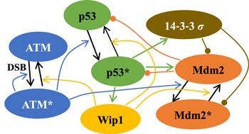
The core of the model is the negative feedback between p53 and Mdm2, that is, p53 promotes the transactivation of Mdm2 gene, but Mdm2 accelerates the degradation rate of p53 via the ubiquitin-proteasome pathway [4]. After DNA double-strand break, ATM quickly senses DNA damage and is activated to a phosphorylated form [12]. The activated ATM can further promote self-activation and the phosphorylation of p53 and Mdm2 [24–26]. For p53, ATM-induced phosphorylation enables it to acquire transcription ability and enhance ubiquitination resistance [24], i.e. the activity and stability of p53 are improved; For Mdm2, ATM-induced phosphorylation makes it more susceptible to self-degradation, and its E3 ubiquitin ligases function is lost [25]. Activated p53 can induce the expression of Wip1, which stands on the opposite side of ATM: the proteins phosphorylated by ATM are restored by Wip1 in our model [13]. Therefore, Wip1 participates in at least two pathways to reduce the activity of p53: (i) promoting dephosphorylation of p53 is a direct pathway, and (ii) promoting dephosphorylation of ATM is an indirect pathway. In addition, Wip1 is also involved in reducing the stability of p53: promoting the dephosphorylation of Mdm2 leads to the stabilization of Mdm2 and the restoration of Mdm2's E3 ubiquitinase function, those are not conducive to the stable existence of p53 [13, 27]. 14-3-3 Σ, another target protein of p53 that is antagonistic to Wip1 by promoting the degradation of Mdm2 [11]. These proteins form the protein signal network shown in figure 1. It is difficult to intuitively understand the dynamics of p53 without a mathematical model.

Figure 1.

New window|Download| PPT slide
Figure 1.Schematic diagram of the network model. Promotion and state transition is represented by colored and black arrow-headed lines respectively. The promotion of degradation is indicated by cycle-headed lines.


Without considering the interaction between different substrates, the basic equations (1)–(8) can be written by using the law of mass action, i.e. the reaction P → P^* can be expressed as a function term: k[P], where [P] represents the dimensionless concentration of protein P; P^* stands for the protein P with a phosphate group; k is the reaction rate.• The form of ATM switches between active and inactive, but their total amount is almost unchanged [26]. These facts make the kinetic terms of ATM’s generation and degradation are not included in the model, which is the main difference between ATM’s equations and other substances
(1)$\begin{eqnarray}\displaystyle \frac{{\rm{d}}[{\mathrm{ATM}}^{* }]}{{\rm{d}}t}={\overline{k}}_{\mathrm{patm}}[\mathrm{ATM}]-{\overline{k}}_{\mathrm{qatm}}[{\mathrm{ATM}}^{* }].\end{eqnarray}$(2)$\begin{eqnarray}[\mathrm{ATM}]=\mathrm{ATMt}-[{\mathrm{ATM}}^{* }].\end{eqnarray}$• Under resting conditions, p53 is rapidly degraded after production [4]. In other words, inactive p53 has poor stability. After DNA damage, p53 is activated into a stable phosphorylated form [24]. Therefore, the equation of p53 should consist of birth, death, activation, and deactivation dynamic terms The degradation rate of p53 should be greater than that of p53^*, so we set ${\bar{d}}_{{\rm{p}}53}\gg {k}_{1}{\bar{d}}_{{\rm{p}}53}$
(3)$\begin{eqnarray}\displaystyle \frac{{\rm{d}}[{\rm{p}}53]}{{\rm{d}}t}={s}_{{\rm{p}}53}-{\overline{k}}_{\mathrm{pp}53}[{\rm{p}}53]+{\overline{k}}_{\mathrm{qp}53}[{\rm{p}}{53}^{* }]-{\overline{d}}_{{\rm{p}}53}[{\rm{p}}53].\end{eqnarray}$(4)$\begin{eqnarray}\displaystyle \frac{{\rm{d}}[{\rm{p}}{53}^{* }]}{{\rm{d}}t}={\overline{k}}_{\mathrm{pp}53}[{\rm{p}}53]-{\overline{k}}_{\mathrm{qp}53}[{\rm{p}}{53}^{* }]-{k}_{1}{\overline{d}}_{{\rm{p}}53}[{\rm{p}}{53}^{* }].\end{eqnarray}$• Interestingly, Mdm2, the main negative regulator of p53, changes exactly the ‘opposite’ to that of p53 after DNA damage. The ‘opposite’ here refers to stability and enzyme activity, i.e. the phosphorylated Mdm2 induced by DNA damage is rapidly degraded on the one hand, and the effect of Mdm2^* ubiquitin ligase is weakened on the other hand [25]. In the kinetic equations, the degradation rate of Mdm2 should be much smaller than that of Mdm2^*, i.e. ${\bar{d}}_{\mathrm{mdm}2}\ll {k}_{2}{\bar{d}}_{\mathrm{pmdm}2}$. Besides, the kinetic terms in the Mdm2 equations are similar to those of p53.
(5)$\begin{eqnarray}\begin{array}{rcl}\displaystyle \frac{{\rm{d}}[\mathrm{Mdm}2]}{{\rm{d}}t} & = & {\overline{s}}_{\mathrm{mdm}2}-{\overline{k}}_{\mathrm{pmdm}2}[\mathrm{Mdm}2]\\ & & +{\overline{k}}_{\mathrm{qmdm}2}[\mathrm{Mdm}{2}^{* }]-{\overline{d}}_{\mathrm{mdm}2}[\mathrm{Mdm}2].\end{array}\end{eqnarray}$(6)$\begin{eqnarray}\begin{array}{rcl}\displaystyle \frac{{\rm{d}}[\mathrm{Mdm}{2}^{* }]}{{\rm{d}}t} & = & {\overline{k}}_{\mathrm{pmdm}2}[\mathrm{Mdm}2]\\ & & -{\overline{k}}_{\mathrm{qmdm}2}[\mathrm{Mdm}{2}^{* }]-{k}_{2}{\overline{d}}_{\mathrm{mdm}2}[\mathrm{Mdm}{2}^{* }].\end{array}\end{eqnarray}$• Without involving complex situations, the equations of Wip1 and 14-3-3 Σ only contain a synthesis term and a degradation term
(7)$\begin{eqnarray}\displaystyle \frac{{\rm{d}}[\mathrm{Wip}1]}{{\rm{d}}t}={\overline{s}}_{\mathrm{wip}1}-{d}_{\mathrm{wip}1}[\mathrm{Wip}1].\end{eqnarray}$(8)$\begin{eqnarray}\displaystyle \frac{{\rm{d}}[14-3-3\ \sigma ]}{{\rm{d}}t}={\overline{s}}_{14-3-3\sigma }-{d}_{14-3-3\sigma }[14-3-3\ \sigma ].\end{eqnarray}$

When the mutual regulation relationship within the protein components in the network shown in figure 1 is introduced into the model, some reaction rate parameters should be replaced by a generalized Hill function [28]. That is, the reaction ${{\rm{P}}}_{1}\mathop{\to }\limits^{{\rm{P}}}{{\rm{P}}}_{2}$ (P catalyzes the conversion of P₁ into P₂) is expressed as a dynamical term $v\left(1-\rho +\rho \tfrac{{{\rm{P}}}^{n}}{{j}^{n}+{{\rm{P}}}^{n}}\right)$ in the equation. Here, v is the maximum reaction rate, ρ (0 ≤ ρ ≤ 1) is a proportional constant characterizing the dependence degree of the reaction on the enzyme, j represents the half-saturated concentration of the enzyme, and n is the Hill coefficient determined by the number of enzyme molecules in polymers. Since enzymes can significantly improve the reaction efficiency, we set ρ ≥ 0.9. Active monomer ATM plays a catalytic role [26], so its Hill coefficient is 1. P53 acts as a transcription factor in a tetramer form [29], thus the Hill coefficient of p53* is 4. It is assumed that the Hill index of Wip1 and 14-3-3 Σ are 1 and 2, respectively. The subfunctions of the equations (1)–(8) are as follows equations (9)–(19):(9)$\begin{eqnarray}{\overline{k}}_{\mathrm{patm}}={k}_{\mathrm{patm}}\left(1-{\rho }_{0}+{\rho }_{0}\displaystyle \frac{[{\mathrm{ATM}}^{* }]}{{j}_{0}+[{\mathrm{ATM}}^{* }]}\right),\end{eqnarray}$(10)$\begin{eqnarray}{\overline{k}}_{\mathrm{qatm}}={k}_{\mathrm{qatm}}\left(1-{\rho }_{1}+{\rho }_{1}\displaystyle \frac{[\mathrm{Wip}1]}{{j}_{1}+[\mathrm{Wip}1]}\right),\end{eqnarray}$(11)$\begin{eqnarray}{\overline{k}}_{\mathrm{qp}53}={k}_{\mathrm{qp}53}\left(1-{\rho }_{2}+{\rho }_{2}\displaystyle \frac{[\mathrm{Wip}1]}{{j}_{2}+[\mathrm{Wip}1]}\right),\end{eqnarray}$(12)$\begin{eqnarray}{\overline{k}}_{\mathrm{pp}53}={k}_{\mathrm{pp}53}\left(1-{\rho }_{3}+{\rho }_{3}\displaystyle \frac{[{\mathrm{ATM}}^{* }]}{{j}_{3}+[{\mathrm{ATM}}^{* }]}\right),\end{eqnarray}$(13)$\begin{eqnarray}{\overline{d}}_{{\rm{p}}53}={d}_{{\rm{p}}53}\left(1-{\rho }_{4}+{\rho }_{4}\displaystyle \frac{[\mathrm{Mdm}2]}{{j}_{4}+[\mathrm{Mdm}2]}\right),\end{eqnarray}$(14)$\begin{eqnarray}{\overline{s}}_{\mathrm{mdm}2}={s}_{\mathrm{mdm}2}\left(1-{\rho }_{5}+{\rho }_{5}\displaystyle \frac{{[p{53}^{* }]}^{4}}{{j}_{5}^{4}+{[p{53}^{* }]}^{4}}\right),\end{eqnarray}$(15)$\begin{eqnarray}{\overline{k}}_{\mathrm{qmdm}2}={k}_{\mathrm{qmdm}2}\left(1-{\rho }_{6}+{\rho }_{6}\displaystyle \frac{[\mathrm{Wip}1]}{{j}_{6}+[\mathrm{Wip}1]}\right),\end{eqnarray}$(16)$\begin{eqnarray}{\overline{k}}_{\mathrm{pmdm}2}={k}_{\mathrm{pmdm}2}\left(1-{\rho }_{7}+{\rho }_{7}\displaystyle \frac{[{\mathrm{ATM}}^{* }]}{{j}_{7}+[{\mathrm{ATM}}^{* }]}\right),\end{eqnarray}$(17)$\begin{eqnarray}{\overline{d}}_{\mathrm{mdm}2}={d}_{\mathrm{mdm}2}\left(1-{\rho }_{8}+{\rho }_{8}\displaystyle \frac{{[14-3-3\sigma ]}^{2}}{{j}_{8}^{2}+{[14-3-3\sigma ]}^{2}}\right),\end{eqnarray}$(18)$\begin{eqnarray}{\overline{s}}_{\mathrm{wip}1}={s}_{\mathrm{wip}1}\left(1-{\rho }_{9}+{\rho }_{9}\displaystyle \frac{{[{\rm{p}}{53}^{* }]}^{4}}{{j}_{9}^{4}+{[{\rm{p}}{53}^{* }]}^{4}}\right),\end{eqnarray}$(19)$\begin{eqnarray}{\overline{s}}_{14-3-3\sigma }={s}_{14-3-3\sigma }\left(1-{\rho }_{10}+{\rho }_{10}\displaystyle \frac{{[{\rm{p}}{53}^{* }]}^{4}}{{j}_{10}^{4}+{[{\rm{p}}{53}^{* }]}^{4}}\right).\end{eqnarray}$

Indeed, there are few valid experimental data that can evaluate parameter values. Many mathematical models are for investigating the qualitative mechanism of a certain topological network rather than the quantitative data fitting [30, 31]. Our work is also like this. In order to reproduce the experimental phenomenon, the unknown parameters are obtained by the ‘trial and error’ method. The default parameters are in table 1. The unit of concentration is dimensionless ‘C’, and the unit of time is minutes.


Table 1.
Table 1.Simulation parameters.

Parameter	Description	Value and unit
ATMt	The total level of ATM	5 C
kpatm	Maximum activation rate of ATM	0.25 min−1
ρ0	The proportional weight of ATM* autocatalysis	0.96 –
j0	Half-saturated concentration of ATM* autocatalysis	5 C
kqatm	Maximum inactivation rate of ATM	0.45 min−1
ρ1	The proportional weight of ATM* inactivation catalyzed by Wip1	0.95 –
j1	Half-saturated concentration of Wip1 in the catalytic ATM* deactivation	0.9 C
sp53	Basal production rate of p53	1.2 C · min−1
kqp53	Maximum inactivation rate of p53	0.8 min−1
ρ2	The proportional weight of p53* inactivation catalyzed by Wip1	0.91 –
j2	Half-saturated concentration of Wip1 in the catalytic p53* deactivation	0.9 C
kpp53	Maximum activation rate of p53	1 min−1
ρ3	The proportional weight of p53 activation catalyzed by ATM*	0.96 –
j3	Half-saturated concentration of ATM* in the catalytic p53 activation	5 C
dp53	Maximum degradation rate of p53	2.5 min−1
ρ4	The proportional weight of p53 degradation catalyzed by Mdm2	0.97 –
j4	Half-saturated concentration of Mdm2 in the catalytic p53 degradation	1.5 C
smdm2	Maximum generation rate of Mdm2	4.3 C·min−1
ρ5	The proportional weight of Mdm2 generation catalyzed by p53*	0.95 –
j5	Half-saturated concentration of p53* in the catalytic Mdm2 generation	1.5 C
kqmdm2	Maximum dephosphorylation rate of Mdm2	3 min−1
ρ6	The proportional weight of Mdm2* dephosphorylation catalyzed by Wip1	0.98 –
j6	Half-saturated concentration of Wip1 in the catalytic Mdm2* dephosphorylation	0.9 C
kpmdm2	Maximum phosphorylation rate of Mdm2	2.5 min−1
ρ7	The proportional weight of Mdm2 phosphorylation catalyzed by ATM*	0.96 –
j7	Half-saturated concentration of ATM* in the catalytic Mdm2 phosphorylation	5 C
dmdm2	Maximum degradation rate of Mdm2	1.03 min−1
ρ8	The proportional weight of Mdm2 degradation catalyzed by 14-3-3 Σ	0.93 –
j8	Half-saturated concentration of 14-3-3 Σ in the catalytic Mdm2 degradation	0.7 C
swip1	Maximum synthesis rate of Wip1	0.16 C·min−1
ρ9	The proportional weight of Wip1 generation catalyzed by p53*	0.95 –
j9	Half-saturated concentration of p53* in the catalytic Wip1 generation	0.35 C
dwip1	Basal degradation rate of Wip1	0.013 min−1
s14-3-3 Σ	Maximum synthesis rate of 14-3-3 Σ	0.5 C·min−1
ρ10	The proportional weight of 14-3-3 Σ generation catalyzed by p53*	0.99 –
j10	Half-saturated concentration of p53* in the catalytic 14-3-3 Σ generation	0.4 C
d14-3-3 Σ	Basal degradation rate of 14-3-3 Σ	0.175 min−1
k1	The ratio of p53* to p53 degradation rate	0.1 –
k2	The ratio of Mdm2* to Mdm2 degradation rate	10 -

New window|CSV

The initial values in table 2 are selected as the steady state level of various proteins without DNA damage (in the case of k_patm = 0 ). Numerical analyses are performed by using the softwares OSCILL8 and XPPAUT. In the analysis, the parameter ranges in the one-dimensional bifurcation diagrams were selected the cases that can clearly show the limit cycle. Assume that the minimum rate of a biochemical reaction is 0, and the maximum is about 2 times of the default value.


Table 2.
Table 2.Initial condition.

Protein	Initial	Protein	Initial	Protein	Initial	Protein	Initial	Protein	Initial
ATM*	0 C	ATM	5 C	p53*	0.062 C	p53	0.809 C	Mdm2*	0.097 C
Mdm2	1.942 C	Wip1*	0.627 C	14-3-3 Σ	0.03 C

New window|CSV

3. Results

3.1. Reproduce the dynamic behaviors of p53

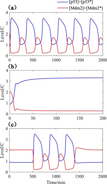
In our theoretical model, DNA damage directly causes ATM activation, which is reflected in the parameter k_patm. The kinetics of p53 is dependent on the DNA damage dose in an environment of permanent stimulation [9]. When a chemotherapy drug, Etoposide, is used as the DNA-damage stimulus, only an appropriate drug dose can trigger p53 oscillations. Thereby, we carried out the experiments in silico as shown in figures 2(a) and (b), and found that excessive DNA damage can totally destroy the dynamic behavior of p53 pulses, which is consistent with biological experiments [9]. Ionizing irradiation is another stimulus type that can trigger p53 oscillations. Different from the treatment with Etoposide solution, ionizing irradiation is a transient pressure on cells, which results in countable p53 pulses [32]. In a hybrid mathematical model of p53, the DNA repair process after radiation is characterized by using Monte Carlo methods: k_patm is almost fixed during DNA repair and the time spent by DNA repair is roughly proportional to the radiation dose [33]. Therefore, we assume that the cell is exposed to radiation at t = 500 min, and it takes 900 min to complete DNA repair. Simulation results are shown in figure 2(c), the p53-Mdm2 module generates three pulses in this case, which is in agreement with the role of p53-Mdm2 feedback loop as a ‘digital’ clock [32]. Furthermore, the experimental phenomenons that DNA damage induces Mdm2's destabilization and the pulse of Mdm2 follows the pulse of p53 also appeared in our numerical simulations [32, 34].

Figure 2.

New window|Download| PPT slide
Figure 2.Time evolution diagram of total p53 (blue line) and total Mdm2 (red line). (a) k_patm = 0.25; (b) k_patm = 0.5; (c) k_patm = 0.25 if $t\in [500,1400]\quad \min $, else, k_patm = 0.


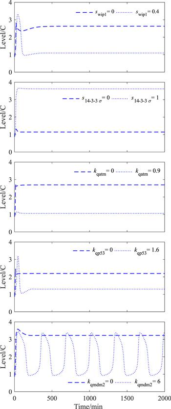
Additionally, it has been experimentally found that the level of p53 induction decreased in Wip1 overexpression cells; in contrast, p53 can reach a high level in the cells treated with Wip1 RNA inhibitor during the DNA damage period [12]. In figure 3, we reproduced these two points by adjusting the Wip1 synthesis rate parameter s_wip1. 14-3-3 Σ positively regulates p53 level [11]. In agreement with its role, figure 3 indicates that the absence of 14-3-3 Σ may lead p53 to approach the basal level, while the enrichment of 14-3-3 Σ can create a high steady state of p53. One might be curious, which of the three arms of Wip1 inhibiting p53 activity and stability is dominant in mediating p53 levels? The answer given by figure 3 is that, the lower level of the p53 steady state is determined by the Wip1-ATM arm or the Wip1-p53 arm, while the higher level of the p53 steady state is determined by the Wip1-Mdm2 arm. When the Wip1-regulated dephosphorylation rate of ATM, p53, or Mdm2 doubles, the lower level of p53 appears in the first two scenarios. And when the biochemical reaction of Wip1-regulated dephosphorylation of ATM, p53, or Mdm2 is removed, the highest level of p53 occurs in the last one scenario. Note that the increase in k_qmdm2 does not affect the p53 oscillation, we will study this issue in the next section.

Figure 3.

New window|Download| PPT slide
Figure 3.Time evolution diagrams of total p53 ([p53] + [p53*]) in some special situations.

3.2. Robustness of oscillation to parameters variation

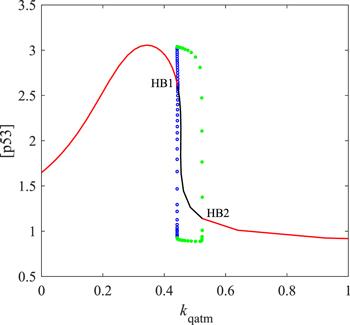
We have explained the feasibility of the model. To our knowledge, oscillation is dependent on the topology of the gene network, the form of regulation function, and parameter selection. Hence, it is necessary to test the sensitivity of oscillation to parameters. In our theoretical model, the oscillation is confined to the parameter interval between two HBs in figure 4. In the second column of table 3, the value range of the parameter that can make p53 oscillate is given as HB1–HB2. It should be noted that when HB is not in the range of physical significance, take the maximum/minimum value with physical significance, that is, for ρ, HB2 on the right side of the oscillation interval is not greater than 1, and for all parameters, HB1 on the left side of the oscillation interval is not less than 0. If only the size of the parameter range where the oscillation occurs is compared, the robustness conclusion obtained is unreliable. For example, the acceptable interval length of ATMt is much larger than k_patm. However, compared with k_patm, ATMt is inherently large, so it is not accurate to claim that ATMt is more robust than k_patm for p53 oscillations. It seems more reasonable to compare the percentage ranges in which the default parameters can be increased (Id%) or decreased (Dd%). From this view, ATMt is a sensitive parameter, compared with k_patm. In the third column of table 3, the Dd% of k_patm is bigger than that of ATMt. Interestingly, the Dd% values corresponding to ρ₆ and j₆ are 100%, which means that the oscillation of p53 is completely independent of Wip1's regulation on Mdm2. Indeed, Wip1's role in Mdm2 dephosphorylation is ignored in many p53 oscillator models [35, 36].

Figure 4.

New window|Download| PPT slide
Figure 4.Codimensional 1 bifurcation diagram. HB represents the Hopf bifurcation point; the red line is the stable equilibrium state; the black line is the unstable equilibrium state. The green dots are the upper and lower bounds of the stable limit cycles; the blue cycles are the upper and lower bounds of the unstable limit cycles.



Table 3.
Table 3.Robustness analysis of p53 oscillations.

Parameter	Oscillation range	Dd%	Id%	S
ATMt	4.332–5.060	13.36%	1.20%	7.75%
kpatm	0.214–0.253	14.40%	1.20%	8.35%
ρ0	0.959–0.977	0.10%	17.71%	0.93%
j0	4.883–6.614	2.34%	32.28%	15.06%
kqatm	0.444–0.524	1.33%	16.44%	8.26%
ρ1	0.665–1.000	30.00%	5.26%	20.12%
j1	0.534–0.985	40.67%	9.44%	29.69%
sp53	0.934–1.217	22.17%	1.42%	13.16%
kqp53	0.787–1.060	1.63%	32.5%	14.78%
ρ2	0.301–1.000	66.92%	9.89%	53.73%
j2	0.216–1.009	76.00%	12.11%	64.73%
kpp53	0.774–1.015	22.60%	1.50%	13.47%
ρ3	0.959–0.991	0.10%	3.23%	1.64%
j3	4.863–7.715	2.74%	54.30%	22.67%
dp53	2.466–3.135	1.36%	25.40%	11.94%
ρ4	0.882–0.973	9.07%	0.31%	4.91%
j4	1.079–1.529	28.07%	1.93%	17.25%
smdm2	4.218–5.976	1.91%	38.98%	17.25%
ρ5	0.930–0.951	2.11%	0.11%	1.12%
j5	0.651–2.073	56.60%	38.20%	52.20%
kqmdm2	2.231–12.266	15.63%	308.87%	69.22%
ρ6	0.000–1.000	100%	2.04%	100.00%
j6	0.000–3.095	100%	243.89%	100.00%
kpmdm2	0.977–2.723	60.92%	8.92%	47.19%
ρ7	0.951–1.000	0.94%	4.17%	2.51%
j7	4.269–50.336	14.62%	906.72%	84.36%
dmdm2	0.691–1.054	32.91%	2.33%	20.80%
ρ8	0.906–0.995	2.58%	6.99%	4.68%
j8	0.682–0.923	2.57%	31.86%	15.02%
swip1	0.152–0.216	5.00%	35.00%	17.39%
ρ9	0.903–0.985	4.95%	3.68%	4.34%
j9	0.308–0.358	12.00%	2.29%	7.51%
dwip1	0.009–0.014	30.77%	7.69%	21.74%
s14-3-3 Σ	0.379–0.513	24.20%	2.60%	15.02%
ρ10	0.982–1.000	0.81%	1.01%	0.91%
j10	0.397–0.434	0.75%	8.50%	4.45%
d14-3-3 Σ	0.171–0.235	2.29%	34.29%	15.76%
k1	0.082–0.313	18.00%	213.00%	58.48%
k2	2.554–13.447	74.46%	34.47%	68.08%

New window|CSV

In addition, the ranges in which some parameters can be increased or decreased is extremely unbalanced. For example, the range of ρ₆ can be increased or decreased to 2.04% or 100%, respectively. It is still not very convenient to study the global robustness. Here, we define S = (HB2 − HB1)/(HB2 + HB1) to describe the sensitivity of oscillation behavior to parameters. Obviously, the ideal (most robust) parameter value is (HB1+HB2)/2, and half the length of the oscillation interval is (HB2-HB1)/2. The larger the S value corresponding to a certain parameter is, the less sensitive the oscillation is to the relative variation of this parameter under the ideal condition. Our calculation results are shown in table 3 fifth column. Approximately 66% of the parameters have an S value of more than 10%, indicating the robustness of this oscillator to the parameter set.

3.3. Dynamics of p53-Mdm2 module regulated by 14-3-3 Σ and Wip1

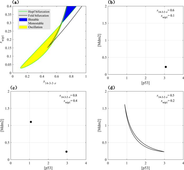
Figure 5 exhibits the dynamic behaviors of the system under the common regulation of Wip1 and 14-3-3 Σ. The parameter plane stretched by the production rates of these two proteins is roughly divided into three types of regions by the two types of bifurcation curves in figure 5(a). Here, roughness mainly means that only the Fold bifurcation and the Hopf bifurcation of the steady-state branch are displayed, while the bifurcations of the limit cycle oscillation branch are ignored, such as the Fold bifurcation of the limit cycle oscillation. We do this omission because the bifurcation curves of the limit cycle oscillation branch are too close to the Hopf bifurcation curve. In the white parameter area, the system will eventually converge to a unique steady state, regardless of the initial state. As shown in the pseudo-phase plane of figure 5(b), there is only one stable fixed point. In the blue parameter area, the system can finally converge to two steady states, and the initial state determines the final steady state of the system. As shown in the pseudo-phase plane of figure 5(c), there are two stable fixed points. In the yellow parameter area, the system will eventually have lasting and stable limit cycle oscillation dynamics, regardless of the initial state. As shown in the pseudo-phase plane of figure 5(d), there is a stable limit cycle. Interestingly, the Fold bifurcation represented by the black line seems to have no contribution to the division of the dynamic regions. In fact, the Fold bifurcation is the fundamental reason why the system appears bistable, but the Hopf bifurcation within the two Fold bifurcation points reduces the bistable region. Rigorously, this dynamic system also has the excitable state in the white parameter area, but it beyond our research and is not considered. Clearly, in this theoretical model, the p53 oscillation is generated by the interconnection between Wip1 mediated negative feedback and 14-3-3 Σ mediated positive feedback. This is a typical characteristic of relaxation oscillations.

Figure 5.

New window|Download| PPT slide
Figure 5.(a) Codimension 2 bifurcation diagram. The green line represents the Hopf bifurcation, and the black line represents the Fold bifurcation. The blue area indicates the bistable state; the white area indicates the monostable state; the yellow area indicates the oscillation. (b)–(d) are pseudo-phase plane, black dots represent stable fixed points, and black closed orbit represents stable limit cycle.


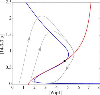
In order to further explain the mechanism of relaxation oscillation, we adopt the pseudo-phase plane analysis method. Firstly, let the right side of equation (7) be zero, that is, [Wip1] degenerates into a parameter; by making a bifurcation curve of [14-3-3 Σ] versus [Wip1], a Z-shaped pseudo-nullcline (zero slope line) can be obtained as shown in figure 6 blue solid line. Secondly, let the right side of equation (8) be zero to get another pseudo-nullcline. The two nullclines intersect in the middle branch of the Z-shaped line, so the fixed point is unstable. After DNA damage, the concentration of 14-3-3 Σ rise rapidly, and the level of Wip1 enhance follow the increase of the concentration of 14-3-3 Σ; when the concentration of Wip1 exceed the right knee of the Z-shaped solid line, the level of 14-3-3 Σ begin to decrease rapidly until nears the lower branch of the Z-shaped solid line; meanwhile, the concentration of Wip1 will decrease to a level below the left knee of the Z-shaped solid line, resulting in the 14-3-3 Σ level rapidly enhance once again. The increase and decrease process of this cycle can create the oscillations of p53. Mathematically, the Folded (Z-shaped) bifurcation curve cannot be separated from the positive feedback. Thereby, besides Wip1-mediated negative feedback, a positive feedback is also required for the relaxation oscillations of p53. Indeed, there are experimental evidences that preliminarily prove that the oscillation of p53 requires both positive and negative feedback. As a negative regulator of p53, Wip1 can significantly affect the occurrence of p53 oscillations has been confirmed experimentally by Batchelor et al [12]; recently, exciting experiments have found that a type of negative regulator of Mdm2 (miR-192, a transactivation target of p53, similar in function to 14-3-3 Σ, can reduce Mdm2 level) also has a constructive effect on the p53 vibrator [37]. As aforementioned, there are many types of bifurcations that can give rise to p53 oscillations [6, 7]. In this model, p53 oscillations can be born from both sup-HB and sub-HB in figure 7. Therefore, there is a great possibility that the oscillation of p53 is a relaxation oscillation, just like our model.

Figure 6.

New window|Download| PPT slide
Figure 6.Pseudo-phase plane analysis. The blue line and red line represent the pseudo-collar slope lines. The gray line indicates orbit. Black dot represents unstable fixed point.

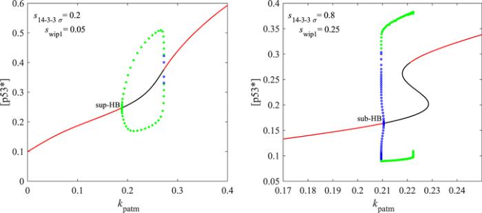
Figure 7.

New window|Download| PPT slide
Figure 7.Codimension 1 bifurcation diagram. sup- or sub- HB represents the supcritical or subcritical Hopf bifurcation point respectively; the red line is the stable equilibrium state; the black line is the unstable equilibrium state. The green dots are the upper and lower bounds of the stable limit cycles; the blue cycles are the upper and lower bounds of the unstable limit cycles.

3.4. Impact of Wip1 and 14-3-3 Σ expression levels on the programmed cell death

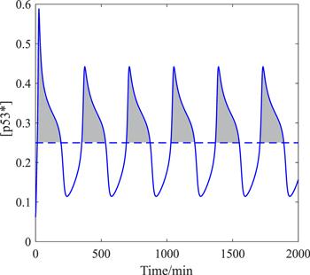
There has been much theoretical work on revealing the relationship between p53 dynamics and cell apoptosis. In the original hypothesis, it was believed that p53 needs to reach a high steady state to initiate apoptosis [38], which is based on the biological knowledge that the binding affinity of p53 to pro-apoptotic genes is weaker than that of pro-survival genes [39]. Latter, two research groups from Nanjing University in China proposed the hypothesis that p53 pulses induce apoptosis: in the model of Sun et al, pro-apoptotic proteins slowly accumulate in p53 pulses until the threshold is reached [40]; in the model of Zhang et al, the post-translational modification of p53 gradually changed from pro-survival to pro-apoptotic [41, 42]. In these models, apoptosis seems to require p53 oscillations peak to be high enough, and the number of p53 pulses to be enough [40–42]. In general, the high steady level of p53 induces faster apoptosis, while the excessive number of p53 pulses causes slower apoptosis. Recently, Wu et al proposed an apoptosis hypothesis, which can explain both the rapid and the slow induction of apoptosis by p53 high steady state and excessive pulses, respectively [43]. For simplicity, this paper adopts the hypothesis of Wu et al.

It is not the absolute accumulation level of p53 that initiates apoptosis, but the effective accumulation level above a certain threshold as the gray area shown in figure 8. In the language of mathematics, the area of the gray area can be expressed as an integral. We define ‘effective cumulative p53’ (ECP [43]) as ECP = ${\int }_{0}^{2000}{\rm{H}}([{\rm{p}}{53}^{* }]-\mathrm{Th})([{\rm{p}}{53}^{* }]-\mathrm{Th}){\rm{d}}t$, where Th is the threshold value, and H(x) is the Heaviside function: ${\rm{H}}(x)=\left\{\begin{array}{l}0\quad x\leqslant 0\\ 1\quad x\gt 0\end{array}\right.$. In the experiments, ECP is positively correlated with the apoptosis rate [43]. Under such an apoptotic mechanism, the pro-apoptotic post-translational modification (such as phosphorylation on Ser-46 [41, 42]) of p53 may lower the threshold value Th. Because Th can also be understood as the threshold of [p53^*] for pro-apoptotic genes transcription [43]. In the following calculations, the value of Th is taken as 0.25. This value is randomly selected between the peak and trough of [p53^*] oscillation in figure 8, because we want to reproduce that the oscillation behavior of p53 also has the potential to induce apoptosis [43].

Figure 8.

New window|Download| PPT slide
Figure 8.The schematic diagram of ECP, the blue solid line is the time history of p53*, the blue dashed line is the threshold Th, and the gray area is the accumulation of p53 that is conducive to apoptosis.


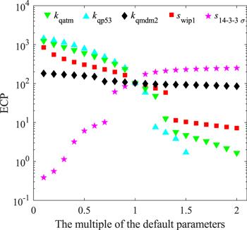
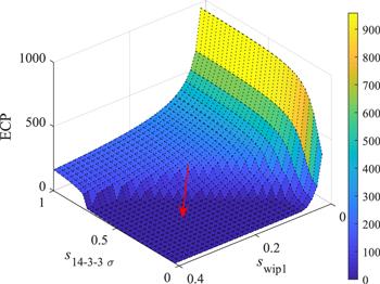
Regardless the dynamic patterns of p53, in the default initial condition, as the level of Wip1 increases, the value of ECP will decrease (red squares in figure 9), and when s_wip1 increases from 1.3 times of the default value to 1.4 times, there is a big gap in ECP, like a switch. It should be noted that the ‘switch’ behavior in here may also change continuously, or equivalent to the so-called ‘ultrasensitive’ [44]. As mentioned above, Wip1 regulates the p53-Mdm2 module through three pathways. Among them, the pathways that directly or indirectly inactivate p53 have a more obvious impact on ECP (figure 9 green and cyan triangles). Our model shows that, like the kinetics of p53 (the indexes of robustness of k_qmdm2 are all relatively high), ECP is not sensitive to the parameter k_qmdm2 (figure 9 black diamonds), which means that Wip1's promotion on Mdm2 stability is not very effective in blocking apoptosis. Contrary to Wip1, as the level of 14-3-3 Σ increases, the value of ECP will increase (figure 9 pink five-pointed stars), and when s_{14-3-3 Σ} increases from 0.7 times of the default value to 0.8 times, the ECP ‘switch’ is ‘toggled open’, and the apoptosis probability is greatly increased. In order to show the mechanism of canceration more intuitively, we make a three-dimensional map as shown in figure 10. The red arrow indicates the direction of canceration. It can be seen that Wip1 level is too high or 14-3-3 Σ level is too low will not be conducive to cell apoptosis. Our results are well in line with the tumor suppressor function of 14-3-3 Σ and the tumor engine function of Wip1.

Figure 9.

New window|Download| PPT slide
Figure 9.The functional relationship between ECP and k_qatm (green inverted triangles), k_qp53 (cyan upright triangles), k_qmdm2 (black diamonds), s_wip1 (red squares), and s_14-3-3Σ (pink five-pointed stars).

Figure 10.

New window|Download| PPT slide
Figure 10.ECP as a function of s_wip1 and s_14-3-3Σ. The colors indicate the value of ECP, as the color bar on the right. The red arrow points to the direction of canceration.

4. Conclusion and discussion

In summary, this article uses the ordinary differential equation dynamics model to study the physiological phenomena of dynamics in the p53 protein signal network and apoptosis underlying p53 dynamics. Our innovation lies in exploring the simultaneous effects of 14-3-3 Σ and Wip1 on the p53-Mdm2 module. We explained the reason of p53 oscillation, that is, the relaxation oscillation caused by the interconnection of 14-3-3 Σ mediated positive and Wip1 mediated negative feedbacks, and explained the roles of Wip1 and 14-3-3 Σ in apoptosis, that is, the accumulation of active p53 exceeding the threshold within a certain period of time will be down-regulated by Wip1 and up-regulated by 14-3-3 Σ. Tumor cells often have strong proliferation ability but weak apoptosis ability. We explained the tumor-promoting function of Wip1 and the tumor-inhibiting function of 14-3-3 Σ from the perspective of apoptosis. As for cancer suppression strategies, targeting Wip1 axis and 14-3-3 Σ axis at the same time may be a more optimized approach.

Note that in the experiments of Wu et al [43], Bax is activated when apoptosis occurs, which is consistent with the model prediction of Sun et al [40]; the concentration of p53 increases significantly when apoptosis is initiated, which is consistent with the model prediction of Zhang et al [42]. From the aspect that the p53 concentration burst during the apoptotic phase, the model of Wee et al is also reasonable [38]. In the mitochondrial apoptotic pathway, Bax inserts into the outer mitochondrial membrane, enhances the permeability of the mitochondrial membrane, releases cytochrome C, and then forms a positive feedback with caspase 3 to amplify the apoptotic signal cascade [45, 46]. In the simplified mathematical models, a certain step in these processes can be selected as an apoptotic marker [40–42]. In our view, ‘ECP’ can be a key indicator in these models of crosstalk between p53 module and apoptotic module if Th is selected to a proper value. We think that it is also meaningful work to establish more computational models for the network motifs downstream of p53, similar to [31]. Moreover, whether the similar-switch behaviors in the figure 9 are continuous is an open question for the readers.

Undoubtedly, this paper has some significance for understanding the roles of Wip1 and 14-3-3 Σ in the p53 protein signaling network, but there are also some shortcomings at the same time. For model building, a partial differential equation model with spatial distribution can be considered [47], a stochastic differential equation model with internal or external noise can be considered [35], and so on. For cellular results, there are actually more options besides apoptosis, such as DNA repair guided by p53 dynamics [40, 41], cell cycle arrest guided by p53 dynamics [41, 42], senescence guided by p53 dynamics [8], etc. In addition, due to the high dimensionality of the model, only numerical calculations have been applied. In the future, we will reduce the dimensionality of the model to facilitate the application of more mathematical theoretical methods, such as the linear stability analysis and bifurcation theory [48], to better understand the relaxation oscillation of p53. We hope that this work can provide some enlightenment to researchers in related disciplines.

Acknowledgments

The authors are very grateful for the professional and detailed suggestions of the anonymous reviewers.

Reference View Option By original order
By published year
By cited within times
By Impact factor

[1]Shabestari P S Rostami Z Pham V Alsaadi F E Hayat T 2019 Commun. Theor. Phys. 71 1241
DOI:10.1088/0253-6102/71/10/1241 [Cited within: 1]

[2]He L Zhu L 2021 Commun. Theor. Phys. 73 035002
DOI:10.1088/1572-9494/abd84a [Cited within: 1]

[3]Hiroaki K 2002 Science 295 1662
DOI:10.1126/science.1069492 [Cited within: 1]

[4]Lev B Maya R Segel L Alon U Levine A Oren M 2000 Proc. Natl Acad. Sci. USA 97 11250
DOI:10.1073/pnas.210171597 [Cited within: 3]

[5]Geva-Zatorsky N et al. 2006 Mol. Syst. Biol. 2 2006.0033
DOI:10.1038/msb4100068 [Cited within: 1]

[6]Hat B Puszynski K Lipniacki T 2009 IET Syst. Biol. 3 342
DOI:10.1049/iet-syb.2008.0156 [Cited within: 3]

[7]Tyson J 2006 Mol. Syst. Biol. 2 0032
DOI:10.1038/msb4100060 [Cited within: 2]

[8]Purvis J E Karhohs K W Mock C Batchelor E Loewer A Lahav G 2012 Science 332 1440
DOI:10.1126/science.1218351 [Cited within: 2]

[9]Chen X Chen J Gan S Guan H Zhou Y Ouyang Q Shi J 2013 BMC Biol. 11 1
DOI:10.1186/1741-7007-11-1 [Cited within: 3]

[10]Hermeking H Lengauer C Polyak K He T C Zhang L Thiagalingam S Kinzler K W Vogelstein B 1997 Mol. Cell 1 3
DOI:10.1016/S1097-2765(00)80002-7 [Cited within: 1]

[11]Yang H Y Wen Y Y Chen C H Lozano G Lee M H 2003 Mol. Cell Biol. 23 7096
DOI:10.1128/MCB.23.20.7096-7107.2003 [Cited within: 3]

[12]Batchelor E Mock C S Bhan I Loewer A Lahav G 2008 Mol. Cell 30 277
DOI:10.1016/j.molcel.2008.03.016 [Cited within: 4]

[13]Shimada M Nakanishi M 2013 Front. Oncol. 3 8
DOI:10.3389/fonc.2013.00008 [Cited within: 3]

[14]Vogelstein B Lane D Levine A 2000 Nature 408 307
DOI:10.1038/35042675 [Cited within: 1]

[15]Ferguson A T Evron E Umbricht C B 2000 Proc. Natl Acad. Sci. USA 97 6049
DOI:10.1073/pnas.100566997 [Cited within: 1]

[16]Akahira J 2004 Clin. Cancer Res. 10 2687
DOI:10.1158/1078-0432.CCR-03-0510 [Cited within: 1]

[17]Uchida D Begum N Almofti A Kawamata H Yoshida H Sato M 2004 Br. J. Cancer 91 1131
DOI:10.1038/sj.bjc.6602004 [Cited within: 1]

[18]Suzuki H Itoh F Toyota M Kikuchi T Kakiuchi H Kohzoh I 2000 Cancer Res. 60 4353
[Cited within: 1]

[19]Lodygin D Diebold J Hermeking H 2004 Oncogene 23 9034
DOI:10.1038/sj.onc.1208004 [Cited within: 1]

[20]Osada H Tatematsu Y Yatabe Y Nakagawa T Konishi H Harano T Tezel E Takada M Takahashi T 2002 Oncogene 21 2418
DOI:10.1038/sj.onc.1205303 [Cited within: 1]

[21]Li J et al. 2002 Nat. Genet. 31 133
DOI:10.1038/ng888 [Cited within: 1]

[22]Rauta J Alarmo E L Kauraniemi P Karhu R Kuukasjarvi T Kallioniemi A 2006 Breast Cancer Res. Treat. 95 257
DOI:10.1007/s10549-005-9017-7 [Cited within: 1]

[23]Saito-Ohara F Imoto I Inoue J Hosoi H Inazawa J 2003 Cancer Res. 63 1876
[Cited within: 1]

[24]Chehab N Malikzay A Malikzay A Stavridi E S Halazonetis T D 1999 Proc. Natl Acad. Sci. USA 96 13777
DOI:10.1073/pnas.96.24.13777 [Cited within: 3]

[25]Magnussen H et al. 2020 Nat. Commun. 11 2094
DOI:10.1038/s41467-020-15783-y [Cited within: 2]

[26]Bakkenist C Kastan M 2003 Nature 421 499
DOI:10.1038/nature01368 [Cited within: 3]

[27]Lu X Ma O Nguyen T A Jones S N Oren M Donehower L A 2007 Cancer Cell 12 342
DOI:10.1016/j.ccr.2007.08.033 [Cited within: 1]

[28]Zhuge C Sun X Chen Y Lei J 2016 J. Theor. Biol. 388 1
DOI:10.1016/j.jtbi.2015.09.025 [Cited within: 1]

[29]Jeffrey P Gorina S Pavletich N 1995 Science 267 1498
DOI:10.1126/science.7878469 [Cited within: 1]

[30]Liu N Yang H Yang L 2021 Commun. Theor. Phys. 73 035601
DOI:10.1088/1572-9494/abd84c [Cited within: 1]

[31]Zhang T Brazhnik P Tyson J 2009 Biophys. J. 97 415
DOI:10.1016/j.bpj.2009.04.053 [Cited within: 2]

[32]Lahav G Rosenfeld N Sigal A Geva-Zatorsky N Levine A J Elowitz M B Alon U 2004 Nat. Genet. 36 147
DOI:10.1038/ng1293 [Cited within: 3]

[33]Ma L Wagner J Rice J J Hu W W Levine A J Stolovitzky G A 2005 Proc. Natl Acad. Sci. USA 102 14266
DOI:10.1073/pnas.0501352102 [Cited within: 1]

[34]Stommel J Wahl G 2004 EMBO J. 23 1547
DOI:10.1038/sj.emboj.7600145 [Cited within: 1]

[35]Wang D G Wang S Huang B Liu F 2019 Sci. Rep. 9 5883
DOI:10.1038/s41598-019-41904-9 [Cited within: 2]

[36]Bi Y Liu Q Wang L Yang W Wu X 2020 Int. J. Bifurcation Chaos 30 2050134
DOI:10.1142/S0218127420501345 [Cited within: 1]

[37]Moore R Kiang Ooi H Kang T Leonidas B Lan M 2015 PLOS Comput. Biol. 11 e1004653
DOI:10.1371/journal.pcbi.1004653 [Cited within: 1]

[38]Wee K Aguda B 2006 Biophys. J. 91 857
DOI:10.1529/biophysj.105.077693 [Cited within: 2]

[39]Weinberg R L Veprintsev D B Bycroft M Fersh A R 2005 J. Mol. Biol. 348 589
DOI:10.1016/j.jmb.2005.03.014 [Cited within: 1]

[40]Sun T Chen C Wu Y Zhang S Cui J Shen P P 2009 BMC Bioinform. 10 190
DOI:10.1186/1471-2105-10-190 [Cited within: 5]

[41]Zhang X P Liu F Cheng Z Wang W 2009 Proc. Natl Acad. Sci. USA 106 12245
DOI:10.1073/pnas.0813088106 [Cited within: 4]

[42]Zhang X P Liu F Wang W 2011 Proc. Natl Acad. Sci. USA 108 8990
DOI:10.1073/pnas.1100600108 [Cited within: 6]

[43]Wu M Hui Y Tang Z Chang S Lu G Chen B Yang Y Wang G Hao H 2017 Cell Death Dis. 8 e3130
DOI:10.1038/cddis.2017.492 [Cited within: 6]

[44]Tian X Huang B Zhang X P Lu M Liu F Onuchic J N Wang W 2017 Proc. Natl Acad. Sci. USA 114 5337
DOI:10.1073/pnas.1702412114 [Cited within: 1]

[45]Schleich K Lavrik I N 2013 Cell Commun. Signal 11 44
DOI:10.1186/1478-811X-11-44 [Cited within: 1]

[46]Kirsch D G et al. 1999 J. Biol. Chem. 274 21155
DOI:10.1074/jbc.274.30.21155 [Cited within: 1]

[47]Elias̆ J Dimitrio L Clairambault J Natalini R 2014 Phys. Biol. 11 045001
DOI:10.1088/1478-3975/11/4/045001 [Cited within: 1]

[48]Zhu L Huang X 2019 Commun. Theor. Phys. 72 015002
DOI:10.1088/1572-9494/ab4ef6 [Cited within: 1]