New holographic Weyl superconductors in Lifshitz gravity
本站小编 Free考研考试/2022-01-02
Jun-Wang Lu,,1,2,∗, Ya-Bo Wu,3, Huai-Fan Li,4, Hao Liao,1, Yong Zheng,1, Bao-Ping Dong,11School of Physics and Electronics, Qiannan Normal University for Nationalities, Duyun 558000, China 2CAS Key Laboratory of Theoretical Physics, Institute of Theoretical Physics, Chinese Academy of Sciences, Beijing 100190, China 3Department of Physics, Liaoning Normal University, Dalian 116029, China 4Department of Physics, Shanxi Datong University, Datong 037009, China
First author contact:∗Author to whom any correspondence should be addressed. Received:2021-01-17Revised:2021-02-9Accepted:2021-02-20Online:2021-03-22
Fund supported:
National Natural Science Foundation of China.11647167 National Natural Science Foundation of China.11747615 National Natural Science Foundation of China.11865012 National Natural Science Foundation of China.12075109 National Natural Science Foundation of China.12075143
Abstract We build holographic p-wave conductor(insulator)/superconductor models via the numerical method with a new form of Weyl coupling in five-dimensional Lifshitz gravity, and then investigate how the Weyl coupling parameter γ and the Lifshitz scaling parameter z affect the superconductor models. In the conductor/superconductor model, an increase in the Weyl correction (Lifshitz scaling) enhances (inhibits) the superconductor phase transition. Meanwhile, both the Weyl correction (when the Lifshitz parameter is large enough and fixed) and the Lifshitz scaling suppress the growth of the real part of the conductivity. The Weyl correction used here (CB2) shows weaker effects on the critical value than the previous Weyl correction (CF2). In the insulator/superconductor model, larger vaules of the Weyl parameter hinder the formation of condensate. However, in increase in the Lifshitz scaling enhances the appearance of condensate. In addition, the calculation suggests that a competitive relation may exist between the Weyl correction and the Lifshitz scaling. Keywords:Weyl correction;Lifshitz gravity;Holographic superconductor
PDF (752KB)MetadataMetricsRelated articlesExportEndNote|Ris|BibtexFavorite Cite this article Jun-Wang Lu, Ya-Bo Wu, Huai-Fan Li, Hao Liao, Yong Zheng, Bao-Ping Dong. New holographic Weyl superconductors in Lifshitz gravity. Communications in Theoretical Physics, 2021, 73(5): 055401- doi:10.1088/1572-9494/abe84a
1. Introduction
Since the gauge/gravity duality was proposed [1, 2], it has been widely applied in various fields of modern physics involving strong interactions [3–9], and, in particular, to high-temperature superconductors [10, 11].
In 2008, a holographic s-wave conductor/superconductor model was first realized by coupling Maxwell’s complex scalar field to Einstein’s gravity in the probe limit [10]. It followed that the model was able to satisfyingly mimic the scalar condensate and infinite DC conductivity as the temperature decreased below the critical value. Subsequently, the holographic superconductor model was further investigated from the perspectives of the magnetic phenomenon [12], departure from the probe limit [13], and the analytical method [14]. The results of these works showed that the holographic tool is indeed an effective and powerful way to probe high-temperature superconductors.
Subsequently, various holographic superconductor models were constructed. For example, to construct superconductors that were closer to the real world and to display more and more of the universal features observed in condensed matter, p- and d-wave conductor (insulator)/superconductor models, superfluids, and multiple order parameters as well as lattice effects were successfully simulated from the holographic perspective [5, 15–27]. To model the anisotropy of spacetime that appears in many real physics systems, a (d + 2)-dimensional non-relativistic gravity with a Lifshitz fixed point was proposed [28, 29], which was then generalized to the finite temperature case (2). Based on the Lifshitz background (2), s- and p-wave conductor(insulator)/superconductor models were constructed in [30–35]. The results showed that for both superconductor models, stronger Lifshitz scaling hinders the superconductor phase transition and suppresses the growth of frequency-dependent conductivity. In addition, via a Maxwell-complex-vector (MCV) field, the authors of [36] realized a magnetic-field-induced condensate, which was confirmed to be a massive generalized version of the SU(2) p-wave model [37–39]. Following this, [22, 24, 40–48] described the construction of electric-field-induced p-wave superconductor models. It followed that the MCV superconductor model displays abundant phase structure in the presence of a back reaction. However, the stronger Lifshitz scaling still makes the superconductor phase transition more difficult.
On the other hand, to broaden the applied range of gauge/gravity duality, many works have focused on the effects of the $\tfrac{1}{\lambda }$(the constant λ denotes the ’t Hooft coupling) correction on holographic superconductor models. In particular, these investigations usually include nonlinear electrodynamic corrections [49, 50] and the higher curvature corrections [38, 51–54] which were found to inhibit the phase transition. In addition, there is another type of correction which involves the combination of the curvature tensor/scalar (or Weyl tensorCμνρσ) and the Maxwell field strength Fμν, for instance, the Weyl form CF2 [55] and its generalized high-derivative version CnF2 [56] as well as the RF2 form [42]. The related superconductor models implied that the MCV p-wave insulator/superconductor model (in particular, the critical chemical potential) is independent of the Weyl correction (CF2). However, the four derivative Weyl (CF2) as well as the six derivative Weyl (C2F2) corrections always promote both the s-wave and MCV p-wave conductor/superconductor models [57–59]. In addition, as one comprehensively takes into account the Lifshitz scaling and the Weyl correction in the MCV superconductor model, both corrections exhibit interesting competitive effects on the critical value and the condensate [60]. In fact, from the viewpoint of effective field theory, apart from the familiar Weyl correction CF2, there are also many other kinds of possible coupling form, such as the coupling ${B}_{\mu \nu }^{\dagger }{C}_{\alpha \beta }^{\mu \nu }{B}^{\alpha \beta }$, where the antisymmetric tensor Bμν is made up of the MCV field ρμ; for details, see the next section. For simplicity, we call this new Weyl correction CB2, to distinguish it from the previous Weyl correction CF2. Bearing in mind the interesting CF2 Weyl effects as well as its competing effects on the Lifshitz scaling of the MCV superconductor [60], in this paper, we will systematically investigate how the CB2 Weyl correction influences the MCV p-wave conductor (insulator)/superconductor models in the Lifshitz black hole (soliton) background. It follows that for some parameter spaces, the influences of the Weyl parameter and the Lifshitz parameter on the conductor/superconductor model are in contrast to their influences on the insulator/superconductor phase transition.
The organization of the rest of this paper is as follows. In section II, we numerically construct a p-wave conductor/superconductor model. Based on a superconducting background, frequency-dependent conductivity is studied. Following a similar procedure, an insulator/superconductor model is built in section III. Conclusions and discussions are summarized in the final section.
2. Conductor/superconductor model
To study the Weyl and Lifshtiz effects on the p-wave conductor/superconductor phase transition, we first introduce the MCV field with the Weyl coupling term CB2 in five-dimensional Lifshitz gravity. The corresponding full action, consisting of the gravitational (${{ \mathcal L }}_{{\rm{g}}}$) and matter (${{ \mathcal L }}_{{\rm{m}}}$) parts reads [28, 29, 36, 40, 41, 56, 61]$\begin{eqnarray}\begin{array}{rcl}S & = & \displaystyle \frac{1}{16\pi {G}_{5}}\displaystyle \int {{\rm{d}}}^{5}x\sqrt{-g}\left({{ \mathcal L }}_{{\rm{g}}}+{{ \mathcal L }}_{{\rm{m}}}\right),\\ {{ \mathcal L }}_{{\rm{g}}} & = & R-2{\rm{\Lambda }}-\displaystyle \frac{1}{2}{\partial }_{\mu }\varphi {\partial }^{\mu }\varphi -\displaystyle \frac{1}{4}{e}^{\iota \varphi }{{ \mathcal F }}_{\mu \nu }{{ \mathcal F }}^{\mu \nu },\\ {{ \mathcal L }}_{{\rm{m}}} & = & -\displaystyle \frac{1}{4}{F}_{\mu \nu }{F}^{\mu \nu }-\displaystyle \frac{1}{4}{B}_{\mu \nu }^{\dagger }({I}_{\alpha \beta }^{\mu \nu }-8\gamma {L}^{2}{C}_{\alpha \beta }^{\mu \nu })\\ & & \times \,{B}^{\alpha \beta }-{m}^{2}{\rho }_{\mu }^{\dagger }{\rho }^{\mu }+{\rm{i}}q{\gamma }_{0}{\rho }_{\mu }{\rho }_{\nu }^{\dagger }{F}^{\mu \nu },\end{array}\end{eqnarray}$where φ, ${{ \mathcal F }}^{\mu \nu }$ in ${{ \mathcal L }}_{{\rm{g}}}$ stand for the massless scalar field and an Abelian gauge field where the parameter ι is related to the Lifshitz dynamic exponent z. The gravitational part ${{ \mathcal L }}_{{\rm{g}}}$ admits the so-called five-dimensional Lifshitz black hole solution as$\begin{eqnarray}\begin{array}{rcl}{\rm{d}}{s}^{2} & = & {L}^{2}\left(-{r}^{2z}f(r){\rm{d}}{t}^{2}+\displaystyle \frac{{\rm{d}}{r}^{2}}{{r}^{2}f(r)}\right.\\ & & +\,\left.{r}^{2}({\rm{d}}{x}^{2}+{\rm{d}}{y}^{2}+{\rm{d}}{w}^{2})\right),f(r)=1-\displaystyle \frac{{r}_{+}^{z+3}}{{r}^{z+3}},\end{array}\end{eqnarray}$where r+ is the location of the event horizon and the Lifshitz parameter z characterizes the degree of anisotropy of spacetime by the scaling symmetry ($t\to {b}^{z}t,r\to {b}^{-1}r,\vec{x}\to b\vec{x}$). Meanwhile, the Hawking temperature is given by $T=\tfrac{(z+3){r}_{+}^{z}}{4\pi }$. The solution of (2) returns standard anti-de Sitter (AdS) spacetime in the case of z = 1. In addition, the matter part ${{ \mathcal L }}_{{\rm{m}}}$ that describes the vector condensate contains a Maxwell field strength Fμν = ∇μAν − ∇νAμ and a vector field ρμ coupled to the Weyl tensor ${C}_{\mu \nu }^{\ \ \ \rho \sigma }$. Specifically, the second-order tensor Bμν = Dμρν − Dνρμ and Dμ = ∇μ − iqAμ. m and q are regarded as the mass and the charge of the vector field ρμ, respectively, and also an identity matrix ${I}_{\mu \nu }^{\ \ \ \rho \sigma }={\delta }_{\mu }^{\ \rho }{\delta }_{\nu }^{\ \sigma }-{\delta }_{\mu }^{\ \sigma }{\delta }_{\nu }^{\ \rho }$. Without losing generality, we will take L = 1. In addition, we construct our model in the probe limit which is still believed to maintain the main characters of superconductors and simplifies the calculation [10, 11, 15, 36].
By a variation of action (1) with respect to the matter fields ρμ and Aμ, respectively, we can write the equations of motion as follows:$\begin{eqnarray}\begin{array}{l}{D}_{\mu }({B}^{\mu \nu }-4\gamma {C}_{\alpha \beta }^{\mu \nu }{B}^{\alpha \beta })\\ \quad -\,{m}^{2}{\rho }^{\nu }+{\rm{i}}{\gamma }_{0}{\rho }_{\mu }{F}^{\mu \nu }=0,\end{array}\end{eqnarray}$$\begin{eqnarray}\begin{array}{l}{{\rm{\nabla }}}_{\mu }({F}^{\mu \nu }-{\rm{i}}{\gamma }_{0}({\rho }^{\mu }{\left({\rho }^{\nu }\right)}^{\dagger }-{\rho }^{\nu }{\left({\rho }^{\mu }\right)}^{\dagger }))\\ \ \ +\,{\rm{i}}({\left({\rho }_{\mu }\right)}^{\dagger }{B}^{\mu \nu }-{\rho }_{\mu }{\left({B}^{\mu \nu }\right)}^{\dagger })\\ \ \ +\,-4{\rm{i}}q\gamma ({\rho }_{\mu }^{\dagger }{C}_{\alpha \beta }^{\mu \nu }{B}^{\alpha \beta }-{\rho }_{\mu }{C}_{\alpha \beta }^{\mu \nu }{\left({B}^{\alpha \beta }\right)}^{\dagger })=0.\end{array}\end{eqnarray}$The above equations have the same form as the equations in [36, 40, 41, 44] when γ = 0 and z = 1 and the equations in [48] when γ = 0 and z ≠ 1.
To build the p-wave superconductor, we turn on the components of the matter fields as described in [36, 40, 41],$\begin{eqnarray}{\rho }_{\nu }{\rm{d}}{x}^{\nu }={\psi }_{x}(r){\rm{d}}x,\ \ \ {A}_{\nu }{\rm{d}}{x}^{\nu }=\phi (r){\rm{d}}t;\end{eqnarray}$substituting this into equations (3) and (4) yields the coupled differential equations for ψx(r) and φ(r). The familiar approach for obtaining the condensate is to solve the differential equations by the shooting method and the imposition of suitable boundary conditions [10, 11, 13, 15, 17, 36]. Specifically, at the horizon (r = r+), we require ψx(r+) to be regular and φ(r+) to be zero to obtain the finite norm of Aμ. At infinity (r → ∞ ), the asymptotical expansions of ψx(r) and φ(r) read$\begin{eqnarray}\begin{array}{rcl}{\psi }_{x}(r) & = & \displaystyle \frac{{\psi }_{1}}{{r}^{{{\rm{\Delta }}}_{-}}}+\displaystyle \frac{{\psi }_{2}}{{r}^{{{\rm{\Delta }}}_{+}}}+\cdots \\ \phi (r) & = & \mu -\displaystyle \frac{\rho }{{r}^{3-z}}+\cdots (z\lt 3),\end{array}\end{eqnarray}$where ${{\rm{\Delta }}}_{\pm }=\tfrac{1}{2}\left(z+1\pm \sqrt{\tfrac{{\left(z+1\right)}^{2}(4z\gamma (z-1)-3)-12{m}^{2}}{4z\gamma (z-1)-3}}\right)$. Compared with the scaling dimension Δ± in [58–60], here, Δ± depends on both Lifshitz and Weyl parameters and thus suggests that the present model might display more interesting features. From the holographic dictionary, ψ1 and ψ2 are usually explained as the source and the vacuum expectation values of the dual operator ${\hat{J}}_{x}$, respectively, while μ and ρ are respectively regarded as the chemical potential and the charge density of boundary field theory. To mimic the spontaneous breaking of U(1) symmetry of the superconductor phase transition, we impose the source-free condition, i.e., ψ1 = 0. Meanwhile, we focus on the Δ = Δ+ = 2 case in this paper, which corresponds to ${m}^{2}=\tfrac{2}{3}(3-2z+4\gamma z-8\gamma {z}^{2}\,+4\gamma {z}^{3})$. In addition, we restrict our calculations to the parameter space where 1 ≤ z < 3 and $\gamma \in \left[-\tfrac{3}{50},\tfrac{2}{50}\right]$, as done in [55, 57, 58]. With the help of the scaling symmetry in the system, we work in the grand canonical ensemble by fixing μ = 1.
Plots of the vector condensate curves for $\gamma =-\tfrac{3}{50},-\tfrac{1}{50}$ and $\tfrac{2}{50}$ are shown in the left(z = 1) and right($z=\tfrac{5}{2}$) panels of figure 1, from which we observe that a critical temperature exists for all cases. Below the critical value, the vector condensate starts to grow. Fitting the curves near the critical point, we find there is always a square-root behavior, such that $\langle {\hat{J}}_{x}\rangle \sim \sqrt{1-\tfrac{T}{{T}_{{\rm{c}}}}}$, which implies that the system may suffer from a second-order phase transition. Meanwhile, when the temperature is decreased, the condensate reaches a saturated value at z = 1 but continuously increases for $z=\tfrac{5}{2}$, which seems to be universal for Lifshitz superconductors [33]. What is more, at the low temperature $\left(\tfrac{{T}_{{\rm{c}}}}{T}\approx \tfrac{1}{5}\right)$, the condensate decreases for z = 1 but increases for $z=\tfrac{5}{2}$ with larger values of γ. By probing the Lifshitz parameter carefully, the location of the demarcation for the qualitatively different behaviors of the condensate is at about ${z}_{d}\approx \tfrac{8}{5}$, where the condensate curves are confirmed to be almost the same for different Weyl parameters $\left(\gamma =-\tfrac{3}{50},0,\tfrac{2}{50}\right)$. Comparing the effects of the new Weyl coupling, CB2, with the one of the previous Weyl couplings, CF2, on the vector condensate, we find that the effect of the new coupling, CB2, is weaker than that of the old Weyl coupling CF2, [60] based on the left panel in figure 1. Furthermore, when γ = 0, the present model is the same as the one in [60] with a vanishing CF2 correction and the model in [42] without an RF2 correction.
Figure 1.
New window|Download| PPT slide Figure 1.The condensate as a function of the temperature corresponding to $\gamma =-\tfrac{3}{50}$ (black solid), 0 (red dashes), $\tfrac{2}{50}$ (blue dots and dashes) for z = 1 (left) and $z=\tfrac{5}{2}$ (right).
In the left panel of figure 2, we display the critical temperature with respect to the Weyl parameter γ for different Lifshitz parameters z, regarding which, we have the following remarks. First of all, when the Weyl parameter γ is fixed and the Lifshitz parameter z increases, the critical temperature clearly decreases, which implies that the improving anisotropy of spacetime hinders the appearance of the vector condensate. The suppressing effect of the Lifshitz scaling on the conductor/superconductor models was also observed in [33, 35, 42, 48]. Secondly, when the Lifshitz parameter z is fixed and the Weyl correction parameter γ gradually increases, the critical temperature increases monotonously, which suggests that the larger the Weyl correction, the more easily the condensate emerges in the conductor/superconductor model. In addition, it is worth mentioning that the critical value increases very slowly with the larger Weyl coupling parameter γ, which again agrees with the weaker influence of the Weyl correction on the condensate in the left panel of figure 1 compared with the left panel of figure 3 in [60]. In addition, for γ = 0, we read off the critical temperatures $\tfrac{{T}_{{\rm{c}}}}{\mu }=0.07958(z=1),0.06133\left(z=\tfrac{3}{2}\right),0.04266(z=2)$ and $0.02244\left(z=\tfrac{5}{2}\right)$, which agree with the corresponding values in the left panel of figure 3 and Tab. 1 in [60]. Last but not least, rescaling the value of ψ2, μ as well as Tc by the charge density ρ, we can translate the system from a grand canonical ensemble with a fixed chemical potential to a canonical ensemble with a fixed charge density; correspondingly, the critical temperature $\tfrac{{T}_{{\rm{c}}}}{\mu }=0.07958$ is rewritten as $\tfrac{{T}_{{\rm{c}}}}{{\rho }^{1/3}}=0.20052$ for the case of z = 1 and γ = 0, which obviously restores to the value in [58] without a CF2 correction.
Figure 2.
New window|Download| PPT slide Figure 2.The left-hand panel displays the critical temperatures for z = 1 (black solid), $\tfrac{3}{2}$ (red dashes), 2 (blue dots and dashes), and $\tfrac{5}{2}$ (purple dots), while the right-hand panel represents the grand potential around the normal state (black dashes) and the superconducting state (red solid) with $z=\tfrac{5}{2}$ and $\gamma =\tfrac{2}{50}$.
Figure 3.
New window|Download| PPT slide Figure 3.The real (solid) and imaginary (dashed) parts of the frequency-dependent conductivity at $\tfrac{T}{{T}_{{\rm{c}}}}\approx \tfrac{1}{5}$ for fixed $\gamma =\tfrac{2}{50}$ with z = 1 (black), $\tfrac{3}{2}$ (red), and $\tfrac{5}{2}$ (blue) in the left-hand panel and for fixed $z=\tfrac{5}{2}$ with $\gamma =-\tfrac{3}{50}$ (black), $-\tfrac{1}{50}$ (red), and $\tfrac{2}{50}$ (blue) in the right-hand panel.
Next, we check the thermodynamic stability as well as the order of the phase transition by calculating the grand potential density of the system $\tfrac{{\rm{\Omega }}}{{V}_{3}}=\tfrac{-{{TS}}_{{\rm{os}}}}{{V}_{3}}$, where Sos is the on-shell action, and V3 = ∫d3x. The on-shell action, given by the Minkowski action (1), is$\begin{eqnarray}\begin{array}{l}{S}_{{\rm{os}}}=\displaystyle \int {{\rm{d}}}^{5}x\displaystyle \frac{\sqrt{-g}}{2}(-{{\rm{\nabla }}}_{\mu }({A}_{\nu }{F}^{\mu \nu }+{\rho }_{\nu }^{\dagger }\\ \ \ \times \,({I}_{\alpha \beta }^{\mu \nu }-8\gamma {C}_{\alpha \beta }^{\mu \nu }){B}^{\alpha \beta })\\ \ \ -\,{\rm{i}}{{qA}}_{\nu }({\rho }_{\mu }^{\dagger }{B}^{\mu \nu }-{\rho }_{\mu }{\left({B}^{\mu \nu }\right)}^{\dagger }))\\ \ \ +\displaystyle \int {{\rm{d}}}^{5}x\sqrt{-g}{\rm{i}}{{qA}}_{\nu }\left(\displaystyle \frac{{\gamma }_{0}}{2}{{\rm{\nabla }}}_{\mu }({\rho }^{\mu }{\rho }^{\nu \dagger }-{\rho }^{\nu }{\rho }^{\mu \dagger })\right.\\ \ \ \left.+\,2\gamma ({\rho }_{\mu }^{\dagger }{C}_{\alpha \beta }^{\mu \nu }{B}^{\alpha \beta }-{\rho }_{\mu }{C}_{\alpha \beta }^{\mu \nu }{\left({B}^{\alpha \beta }\right)}^{\dagger }\right)\\ \ \ =\displaystyle \frac{{V}_{3}}{T}\left(\displaystyle \frac{3-z}{2}\mu \rho -{\displaystyle \int }_{{r}_{+}}^{\infty }\right.\\ \,\times \,\displaystyle \frac{3-4\gamma z(z-1)f-2\gamma (3z-1){{rf}}^{{\prime} }-2\gamma {r}^{2}{f}^{{\prime} ^{\prime} }}{3{r}^{z}f}{\phi }^{2}{\psi }^{2}{\rm{d}}r,\end{array}\end{eqnarray}$where we have taken ∫d3x = V3, $\int {\rm{d}}t=\tfrac{1}{T}$ into consideration and ignored the factor $\tfrac{1}{16\pi {G}_{5}}$. Obviously, both the Weyl parameter γ and the Lifshitz parameter z contribute to the grand potential.
We representatively plot the grand potential versus temperature with $z=\tfrac{5}{2}$ and $\gamma =\tfrac{2}{50}$ in the right-hand panel of figure 2. It follows that at the critical point, the two curves merge smoothly together but not in the form of a swallowtail, which matches the condensed behaviors in figure 1 and, in particular, implies that the phase transition is indeed second order. In addition, the value of the black dashed curve is always larger than that of the red solid curve, which verifies that the hairy state is thermodynamically stable below the critical point. Besides, we have also calculated the behaviors of the grand potential for the other Weyl cases (such as $z=\tfrac{5}{2},\gamma =-\tfrac{3}{50},-\tfrac{2}{50},-\tfrac{1}{50},0,\tfrac{1}{50}$) as well as the other Lifshitz cases ($z=1,\tfrac{3}{2},2,\tfrac{5}{2}$) and obtained similar results to the one in figure 2. Therefore, we believe that our numerical results are quite reliable in the parameter space $\left(1\leqslant z\leqslant \tfrac{5}{2},-\tfrac{3}{50}\leqslant \gamma \leqslant \tfrac{2}{50}\right)$.
In what follows, we take a look at the signals of superconductors, i.e., their infinite DC conductivity, which requires us to calculate the perturbation of the Maxwell field in the bulk from the AdS/conformal field theory (CFT) correspondence. Taking the perturbation along the y direction with the ansatz δAy(t, r)dy = Ay(r)e−iωtdy, and substituting it into equation (4) yields the linearized differential equation of Ay(r) as well as its general falloff as$\begin{eqnarray}{A}_{y}(r)=\left\{\begin{array}{ll}{A}^{(0)}+\tfrac{{A}^{(2)}}{{r}^{2}}+\tfrac{{A}^{(0)}{\omega }^{2}}{2{r}^{2}}\mathrm{ln}\eta r+\cdots , & z=1,\\ {A}^{(0)}+\tfrac{{A}^{(z+1)}}{r}+\cdots , & 1\lt z\lt 3,\end{array}\right.\end{eqnarray}$where A(i), and η are both constants. From equations (1) and (8), the retarded Green’s function reads$\begin{eqnarray}\begin{array}{rcl}G(\omega ) & = & 2\displaystyle \frac{{A}^{(2)}}{{A}^{(0)}}-\displaystyle \frac{1}{2}{\omega }^{2},{\rm{for}}\\ z & = & 1;\ \displaystyle \frac{(z+1){A}^{(z+1)}}{{A}^{(0)}},{\rm{for}}\,1\lt z\lt 3,\end{array}\end{eqnarray}$where the logarithmic divergent term for z = 1 is canceled by the holographic renormalization [11, 33, 42, 60]. By means of the Kubo formula, the frequency-dependent conductivity is given by $\sigma (\omega )=-\tfrac{{\rm{i}}}{\omega }G(\omega )$, from which we can see that the key point in the calculation of the conductivity is to extract the coefficients A(0) and A(z+1) in equation (8). The effective method is still to numerically solve the differential equation of Ay(r) with the ingoing boundary condition at the horizon as ${A}_{y}(r)\,=$${\left(r-{r}_{+}\right)}^{-{\rm{i}}\omega /\left(3+z\right)}\left(1+{A}_{y1}\left(r-{r}_{+}\right)+{A}_{y2}{\left(r-{r}_{+}\right)}^{2}+{A}_{y3}{\left(r-{r}_{+}\right)}^{3}+\cdots \right)$.
We show a typical plot of the AC conductivity at $\tfrac{T}{{T}_{{\rm{c}}}}\approx \tfrac{1}{5}$ for the fixed Weyl parameter $\gamma =\tfrac{2}{50}$ (left) and the Lifshitz parameter $z=\tfrac{5}{2}$(right), respectively, in figure 3. There are clear poles for the imaginary part of the conductivity Im[σ] at the lower frequencies in all cases. From the Kramers-Kronig relation, these poles correspond to a delta function of the real part of the conductivity Re[σ] at the vanishing frequency and thus indicate infinite DC conductivity. Moreover, ${\rm{Re}}[\sigma ]$ increases with frequency and diverges at large frequencies, which is also its universal character in five-dimensional spacetime [11, 33, 42, 60]. Furthermore, in the case of z = 1, there is a minimum for Im[σ] in the intermediate frequency region, which corresponds to the energy gap of the superconductor ωg. After the calculations, we find that the larger the Weyl correction, the smaller the value of $\tfrac{{\omega }_{{\rm{g}}}}{{T}_{{\rm{c}}}}$; for instance, $\tfrac{{\omega }_{{\rm{g}}}}{{T}_{{\rm{c}}}}=8.2821\left(\gamma =-\tfrac{3}{50}\right)$ , $8.1340\left(\gamma =-\tfrac{1}{50}\right),7.9200\left(\gamma =\tfrac{2}{50}\right)$. Meanwhile, the variation of $\tfrac{{\omega }_{{\rm{g}}}}{{T}_{{\rm{c}}}}$ with respect to the Weyl parameter is very slow, which corresponds with the weak Weyl effects on the condensate. As we know, the location of the minimum of Im[σ] corresponds to the frequency region where Re[σ] increases quickly with frequency. As a result, for z = 1, the phenomenon whereby the energy gap moves leftwards with increasing γ corresponding to Re[σ] increases more quickly with larger γ. Interestingly, for a big enough Lifshitz parameter z, such as $z=\tfrac{5}{2}$ on the right-hand panel of figure 3, we find that Re[σ] increases more and more slowly with increases in γ. These different effects of the Lifshitz parameter z on conductivity seem to be consistent with its effects on the condensate shown in figure 1. In addition, as displayed in the left-hand panel of figure 3, Re[σ] is suppressed more and more obviously with an increase in the Lifshitz scaling, which is also observed in [33, 42, 60]. In addition, we also calculated the conductivity for other cases with fixed γ, for example, $\gamma =-\tfrac{3}{50},\,0$ and qualitatively obtained the same results as the ones shown in the left-hand panel of figure 3.
3. Insulator/superconductor model
First of all, by double Wick rotating the Lifshitz black hole (2), i.e., t → iχ and w → it, we read off the five-dimensional Lifshitz soliton$\begin{eqnarray}\begin{array}{rcl}{\rm{d}}{s}^{2} & = & -{r}^{2}{\rm{d}}{t}^{2}+\displaystyle \frac{{\rm{d}}{r}^{2}}{g(r)}+{r}^{2}({\rm{d}}{x}^{2}+{\rm{d}}{y}^{2})+f(r){\rm{d}}{\chi }^{2},\\ f(r) & = & {r}^{2z}\left(1-\displaystyle \frac{{r}_{0}^{z+3}}{{r}^{z+3}}\right),\ g(r)={r}^{2}\left(1-\displaystyle \frac{{r}_{0}^{z+3}}{{r}^{z+3}}\right),\end{array}\end{eqnarray}$where r0 represents the tip f(r0) = 0. In order to guarantee smoothing of the geometry, we have to impose Scherk-Schwarz periodicity ${\rm{\Gamma }}=\tfrac{4\pi }{(z+3){r}_{0}^{z}}$ on the spatial direction χ. As argued in [17], the Lifshitz soliton solution has a negative mass gap, which corresponds to a dual field theory with a mass gap. Due to a similar phenomenon whereby the mass gap also exists in the insulator, the current soliton solution is believed to provide a gravitational background to construct the holographic insulator/superconductor model [17, 33, 41, 58].
Having the Lifshitz soliton background in hand, to build the MCV p-wave superconductor model with the CB2 Weyl correction, we take the Lagrangian density of the matter field ${{ \mathcal L }}_{{\rm{m}}}$ to be equal to the one in equation (1). Considering the same ansatzs of the matter field (5), we can read off the coupled differential equations of motion of ψx(r) and φ(r) in the Lifshitz soliton geometry (10). To numerically solve the differential equations of motion, we add the Neumann-like boundary condition to ψx(r) and φ(r) at the tip; meanwhile the general falloff of ψx(r) is the same as the falloff in equation (6), and the asymptotic solution of φ(r) reads$\begin{eqnarray}\phi (r)=\mu -\displaystyle \frac{\rho }{{r}^{z+1}}+\cdots .\end{eqnarray}$Moreover, the physical translations of the coefficients (ψ1, ψ2, μ and ρ) are the same as the ones in the Lifshitz black hole. In addition, to conveniently compare the models with different parameters, we fix the periodicity Γ = π by rescalling the values of ψ2, μ, and ρ.
After a series of calculations, we display the condensate versus the chemical potential in figure 4 with z = 1 (on the left), $\tfrac{5}{2}$ (on the right), respectively, and the left-hand panel in figure 5 with $\gamma =\tfrac{2}{50}$. Meanwhile, we show the dependence of charge density on the chemical potential with $z=\tfrac{5}{2}$ in the right-hand panel of figure 5. It follows that a critical chemical potential exists for all cases. Above the critical value, the condensate and the charge density appear and then grow monotonously with increasing chemical potential. In particular, near the critical value, all condensates behave according to $\langle {J}_{x}\rangle \sim {(\mu -{\mu }_{{\rm{c}}})}^{\tfrac{1}{2}}$. The critical exponent $\tfrac{1}{2}$ indicates that the system suffers from a second-order phase transition [17, 41]. Meanwhile, the charge density increases linearly, which seems to be a universal property at the probe approximation [17, 33]. What is more, as the Weyl parameter γ increases for z = 1, the critical chemical potential moves towards the right, which implies that the improving Weyl correction inhibits the insulator/superconductor phase transition. On the other hand, the critical chemical value moves towards the left with increasing values of γ for $z=\tfrac{5}{2}$, which suggests the larger the Weyl parameter γ, the easier the phase transition of the system. Obviously, the effects of the Weyl correction on the insulator/superconductor phase transition are quite different from its effects on the conductor/superconductor phase transition. In addition, we observe that the location of the critical chemical potential moves towards the left with improving Lifshitz scaling for $\gamma =\tfrac{2}{50}$, which suggests that stronger Lifshitz scaling allows the insulator/superconductor phase transition to occur more easily.
Figure 4.
New window|Download| PPT slide Figure 4.The condensate for the Weyl parameters $\gamma =-\tfrac{3}{50}$ (black solid), 0 (red dashes), and $\tfrac{2}{50}$ (blue dots and dashes), where $\kappa ={\left(\tfrac{4}{3+z}\right)}^{1/z}$ and the left (right) panel denotes the Lifshitz parameter z = 1 $\left(z=\tfrac{5}{2}\right)$.
Figure 5.
New window|Download| PPT slide Figure 5.The condensate with z = 1 (black solid), $\tfrac{3}{2}$(red dashes), and $\tfrac{5}{2}$(dots and dashes) for $\gamma =\tfrac{2}{50}$ (left) and the charge density with $\gamma =-\tfrac{3}{50}$ (black solid) and 0 (red dashes) and $\tfrac{2}{50}$ (blue dots and dashes) for $z=\tfrac{5}{2}$ (right), where the horizontal axis denotes the chemical potential and the factor $\kappa ={\left(\tfrac{4}{3+z}\right)}^{1/z}$.
Motivated by the above abundant phenomena arising from the Lifshitz and Weyl parameters, we display the critical chemical potential as a function of the Weyl correction with different Lifshitz scaling in figure 6. It can be observed that larger values of γ inhibit the superconductor phase transition for z = 1 and $\tfrac{3}{2}$ and promote the superconductor phase transition for z = 2 and $\tfrac{5}{2}$. Meanwhile, the critical chemical potential varies almost linearly with the Weyl parameter. By calculation, we find that in the $z\approx \tfrac{17}{10}$ case of the Lifshitz parameter, the critical value has nearly no dependence on the Weyl correction. In addition, since the Weyl correction is sufficiently large and fixed, such that $\gamma \geqslant -\tfrac{2}{50}$, the critical value decreases with an increase in the Lifshitz parameter, which means that larger Lifshitz scaling promotes the phase transition. In summary, the Weyl correction and the Lifshitz scaling exhibit competitive behavior in the superconductor model.
Figure 6.
New window|Download| PPT slide Figure 6.The critical chemical potential (left) with z = 1 (black solid), $\tfrac{3}{2}$ (red dashes), 2 (blue dots and dashes), and $\tfrac{5}{2}$ (purple dots) and the grand potential (right) with $z=\tfrac{5}{2}$ for $\gamma =-\tfrac{3}{50}$ (black solid), 0 (red dashes), $\tfrac{2}{50}$ (blue dots and dashes) and the normal state (horizontal dashes), where $\kappa ={\left(\tfrac{4}{3+z}\right)}^{1/z}$.
Similarly to the procedure in section 2, we calculate the grand potential density ($\tfrac{{\rm{\Omega }}}{{V}_{3}}=\tfrac{-{{TS}}_{{\rm{os}}}}{{V}_{3}}$) from the defined ‘temperature’ of the soliton system and the on-shell action. The concrete on-shell action reads$\begin{eqnarray}\begin{array}{l}{S}_{{\rm{os}}}=\displaystyle \frac{{V}_{3}}{T}\left(\displaystyle \frac{1}{2}(z+1)\mu \rho \right.\\ \left.-\,{\displaystyle \int }_{{r}_{0}}^{\infty }\displaystyle \frac{3+4\gamma z(z-1)f+2\gamma (3z-1){{rf}}^{{\prime} }+2\gamma {r}^{2}{f}^{{\prime} ^{\prime} }}{3{r}^{2-z}}{\phi }^{2}{\psi }^{2}{\rm{d}}r\right),\end{array}\end{eqnarray}$which is quite different from the one given in (7) for the black hole. We representatively show the density of the grand potential for $z=\tfrac{5}{2}$ in figure 6. Obviously, as the chemical potential gradually increases from the critical point, all curves with hairy vectors $\left(\gamma =-\tfrac{3}{50},0,\tfrac{2}{50}\right)$ develop smoothly from the horizontal dashed line characterized by no hair. Furthermore, except for the critical point, all hairy curves are always lower than the horizontal line, but do not intersect it, since μ > μc. These characters are not only consistent with the condensed curves in figures 4 and 5, but also indicate that a second-order phase transition occurs at the critical point and the hairy state is thermodynamically stable, which are expected in the superconducting state.
To further check that the hairy state is a superconducting state, it is useful to calculate the conductivity from the investigation of gauge perturbation δAy(t, r) = Ay(r)e−iωt in the hairy bulk. Following the same procedure in the conductor/superconductor model, we read off the linearized differential equation for Ay(r) and further obtain its asymptotic solution as$\begin{eqnarray}\begin{array}{rcl}{A}_{y}(r) & = & {A}^{(0)}+\displaystyle \frac{{A}^{(2)}}{{r}^{2}}+\displaystyle \frac{{A}^{(0)}{\omega }^{2}}{2{r}^{2}}\mathrm{ln}(\eta r){\rm{for}}\\ z & = & 1;{A}^{(0)}+\displaystyle \frac{{\omega }^{2}}{2(z-1)}\displaystyle \frac{{A}^{(0)}}{{r}^{2}}+\displaystyle \frac{{A}^{(z+1)}}{{r}^{z+1}}\,{\rm{for}}\,z\gt 1,\end{array}\end{eqnarray}$the form of which is the same as that shown in [33, 42]. After analysis, we find the concrete expression of the retarded Green’s function related equation (13) is the same as the one for the black hole (9), so that the AC conductivity is again formally equal to the one in the conductor/superconductor model. Given the Neumann-like boundary condition ${A}_{y}(r)=1\,+{{A}_{y1}{(r-{r}_{0})+{A}_{y2}(r-{r}_{0})}^{2}+{A}_{y3}(r-{r}_{0})}^{3}+\cdots $, we can obtain the imaginal part of the conductivity Im[σ] by solving the differential equation for Ay(r). The frequency-dependent conductivity Im[σ] with z = 1 and $z=\tfrac{5}{2}$ at $\tfrac{\mu }{{\mu }_{{\rm{c}}}}\approx 2$ is plotted in figure 7, from which we observe the pole in the low-frequency region. As discussed in the conductor/superconductor model, this pole corresponds to the delta function for Re[σ] and thus indicates infinite DC conductivity, which not only closely matches the behaviors of the condensate and the grand potential, but also provides a signal for the superconductor [17, 33]. What is more, when z = 1, we can see clearly that the curves for the conductivity nearly overlap with each other for $\gamma =-\tfrac{3}{50},\,0,\,\tfrac{2}{50}$. This means that when the chemical potential is sufficiently large, the effects of the CB2 Weyl on the conductivity are rather weak, which is consistent with the phenomenon in figure 4, where the condensate curves for different values of γ tend to coincide at the large chemical potential. Moreover, for a sufficiently large Weyl parameter (such as $\gamma =\tfrac{1}{50}$, not displayed) or Lifshtz scaling, for example, $z=\tfrac{5}{2}$ shown on the right panel of figure 7, the location of the second pole always moves towards the right with the other parameter, z or γ, which seems to agree with the increasing differences of condensates with different parameters in figures 4 and 5.
Figure 7.
New window|Download| PPT slide Figure 7.The imaginary part of the frequency-dependent conductivity $\left(\tfrac{\mu }{{\mu }_{{\rm{c}}}}\approx 2\right)$ for various Weyl parameters: $\gamma =-\tfrac{3}{50}$ (solid), 0 (dashes), and $\tfrac{2}{50}$ (dots and dashes) in the left-hand (z = 1) and right-hand $\left(z=\tfrac{5}{2}\right)$ panels.
4. Conclusions and discussions
In the probe limit, we have numerically built the MCV p-wave conductor/superconductor and insulator/superconductor phase transitions with CB2 Weyl coupling in five-dimensional Lifshitz gravity. We mainly studied the influences of the Weyl (γ) and Lifshitz (z) parameters on the superconductor models. The main results are summarized as follows.
For the conductor/superconductor model, as the Weyl parameter γ increases or the Lifshitz parameter z decreases, the critical temperature becomes larger and larger, which suggests that the phase transition becomes easier and easier with an increase in the Weyl correction or a weakening of the Lifshitz scaling. At low temperatures, as the Weyl parameter increases, the condensate value decreases (increases) below (above) the point of demarcation ${z}_{d}\approx \tfrac{8}{5}$. In addition, we find that Re[σ] grows more and more quickly (slowly) with frequency for smaller(larger) values of z in the intermediate region, which is consistent with the behaviors of the condensate with the corresponding Lifshitz parameter z. Compared with the CF2 Weyl correction [60], the CB2 Weyl correction used here has weaker influences on the condensate and the critical temperature.
For the insulator/superconductor model, as the Weyl parameter increases, the phase transition becomes increasingly difficult (easy) below (above) the point of demarcation ${z}_{d}\approx \tfrac{17}{10}$. Meanwhile, when the Weyl correction is sufficiently strong, the superconductor phase transition becomes increasingly easy with an improvement of the Lifshitz parameter z. On the other hand, compared with the standard case, i.e., z = 1 and γ = 0, we can understand the above results as showing that larger Weyl corrections inhibit the phase transition, while an increase in the Lifshitz scaling enhances the phase transition. Meanwhile, the abundant effects of the Weyl correction and the Lifshitz scaling on the superconductor result from the competition between the two corrections.
In fact, the phenomenon whereby the insulator/superconductor phase transition becomes easier with larger Lifshitz parameters is not strange, and has been observed in the s-wave and MCV p-wave insulator/superconductor models in [33, 42]. In particular, if we redefine the periodicity as Γ = π (with a scaling factor of $\kappa ={\left(\tfrac{4}{3+z}\right)}^{1/z}$) or even the Γ = 2π (with a scaling factor of $\kappa ={\left(\tfrac{2}{3+z}\right)}^{1/z}$) used in [42], we can find the critical value without RF2 correction is the same as the one in the model used here with γ = 0. Meanwhile, for any Weyl and Lifshitz parameters in the range $-\tfrac{3}{50}\leqslant \gamma \leqslant \tfrac{2}{50}$ and $1\leqslant z\leqslant \tfrac{5}{2}$ in the conductor/superconductor model, Re[σ] is always positive though it is very small at low frequencies below the critical temperature, which means that the current superconductor model satisfies the unitary requirement for the present parameter space. Even so, it is meaningful to check whether phenomena such as superluminal velocities or the violation of causality will happen or not for the current Weyl parameter space. In addition, we also calculated the frequency-dependent conductivity near the critical temperature, but did not see the pronounced peak and/or the Drude-like peak that appeared in the case with C2F2 correction [35, 61, 62], so would be interesting to investigate how the sixth-order derivative term C2B2 influences the model. In the near future, we will focus on solving the above problems to improve the understanding of the impact of the Weyl correction on the superconductor model.
Acknowledgments
We would like to thank Prof. L. Li for his helpful discussion. This work is supported in part by NSFC (Grant Nos. 11865012, 12 075 109, 12 075 143 and 11 747 615), the Foundation of Scientific Innovative Research Team of Education Department of Guizhou Province (201329).
 ,
, ,1,2,∗, Ya-Bo Wu
 New window|Download| PPT slide
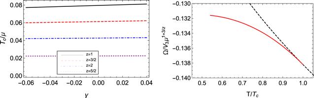 New window|Download| PPT slide
 New window|Download| PPT slide
 New window|Download| PPT slide
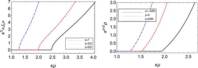 New window|Download| PPT slide
 New window|Download| PPT slide
 New window|Download| PPT slide