Abstract Based on simple combinatorial arguments, we formulate a generalized cavity method where the Random Overlap Structure (ROSt) probability space of Aizenmann, Sims and Starr is obtained in a constructive way, and we use it to give a simplified derivation of the Parisi formula for the free energy of the Sherrington–Kirkpatrick model. Keywords:Sherrington–Kirkpatrick model;cavity methods;Parisi formula
Some decades ago a very sophisticated mean-field (MF) theory was developed by Parisi to compute the thermodynamic properties of the Sherrington–Kirkpatrick (SK) model in the low-temperature phase [1–6]. In his theory, that is obtained within the larger framework of the replica theory [2, 5], Parisi introduced many important concepts that are now standards in the field, like the overlap distribution as an order parameter and the nontrivial hypothesis that the scalar products between independent replicas of the system (overlaps) concentrate on a numeric support that is ultrametrically organized [2, 3, 5, 7–13].
After many years Guerra [3] and Talagrand [4] showed that this remarkable MF theory indeed provides the correct expression for the free energy of the SK model, while Panchenko proved that the SK Gibbs measure can be perturbed into a special cascade of point processes (Ruelle cascade [9, 10]) that gives the same free energy and indeed satisfies the ultrametricity assumption [10, 13]. These mathematical milestones and many other theoretical and numerical tests (see [6] and references) contributed to form the idea that, at least for MF models, this ansatz provides the correct physical properties.
Following simple combinatorial arguments we show that the same results of the replica symmetry breaking (RSB) theory can be obtained in a constructive way without relying on the replica trick, or averaging on the disorder. After presenting a general analysis of the SK Hamiltonian, we will show that the usual assumptions associated with L levels of RSB (see [2, 8–10, 14]) are consistent with a hierarchical MF theory in which the states ensemble is charted according to a sigma algebra generated by a partition of the vertex set. The method provides a constructive derivation of the Random Overlap Structure (ROSt) probability space introduced in [8] by Aizenmann, Sims and Starr. We further tested this by computing the corresponding incremental pressure that one obtains from the cavity method [2, 8, 9], and it indeed provides the correct Parisi functional.
We start by introducing the basic notation. Let us consider a spin system of N spins; we indicate the spin sites by the vertex set $V=\left\{1,2,\ldots ,N\right\}$, marked by the label i. A unique spin variable ${\sigma }_{i}$ that can be plus or minus is associated with each vertex. Formally ${\sigma }_{i}\in {\rm{\Omega }}$, hereafter we assume ${\rm{\Omega }}=\left\{+,\,-\right\}$, although our argument holds for any size of $| {\rm{\Omega }}| $ (for this paper a modulus $| \,\cdot \,| $ applied to a discrete set returns its cardinality, for example $| V| =N$). We collect the spins into the vector$\begin{eqnarray}{\sigma }_{V}=\left\{{\sigma }_{i}\in {\rm{\Omega }}:\,i\in V\right\},\end{eqnarray}$that is supported by the N−spin vector space ${{\rm{\Omega }}}^{V}$, and we call these vectors magnetization states. Notice that we implicitly established an arbitrary reference frame on V by labeling the spins.
Let J be some matrix of entries ${J}_{{ij}}=O\left(1\right)$. Even if the arguments we are going to present are not limited to this case, in the following we also assume that the Jij entries are random and normally distributed. Then, the Sk model without an external field is described by the Hamiltonian$\begin{eqnarray}H\left({\sigma }_{V}\right)=\displaystyle \frac{1}{\sqrt{N}}\displaystyle \sum _{\left(i,j\right)\in W}{\sigma }_{i}{J}_{{ij}}{\sigma }_{j},\end{eqnarray}$where $W=V\otimes V$ is the edges set accounting for the possible spin–spin interactions and $\sqrt{N}$ is a normalization that in MF models can be $| V| -$ dependent. In the SK model the interactions are normally distributed and we have to take a normalization that is the square root of the number of spins $| V| =N$, but the same analysis can be repeated for any coupling matrix and its relative normalization. As usual, we can define the partition function$\begin{eqnarray}{Z}_{N}=\displaystyle \sum _{\sigma \in {{\rm{\Omega }}}^{V}}\exp \left[-\beta H\left({\sigma }_{V}\right)\right],\end{eqnarray}$and the associated Gibbs measure$\begin{eqnarray}\mu \left({\sigma }_{V}\right)=\displaystyle \frac{\exp \left[-\beta H\left({\sigma }_{V}\right)\right]}{{Z}_{N}}.\end{eqnarray}$The free energy density is written in terms of the pressure$\begin{eqnarray}p=\mathop{\mathrm{lim}}\limits_{N\to \infty }\displaystyle \frac{1}{N}\mathrm{log}{Z}_{N},\end{eqnarray}$and the free energy per spin is given by $-p/\beta $.
A variational formula for the pressure of the SK model has been found by Parisi [1]. Following this, and after [2, 8–10] it has been proven that the average pressure per spin can be computed from the relation$\begin{eqnarray}E\left(p\right)=\mathop{\inf }\limits_{q,\lambda }\,{A}_{P}\left(q,\lambda \right),\end{eqnarray}$where ${A}_{P}\left(q,\lambda \right)$ is the Parisi functional of the (asymmetric) SK model, as defined in equation (3); hereafter, for the noise average we use the special notation $E\left(\,\cdot \,\right)$.
The minimizer is taken over two non-decreasing sequences $q=\left\{{q}_{0},{q}_{1},\ldots ,{q}_{L}\right\}$ and $\lambda =\left\{{\lambda }_{0},{\lambda }_{1},\ldots ,{\lambda }_{L}\right\}$ such that ${q}_{0}={\lambda }_{0}=0$ and ${q}_{L}={\lambda }_{L}=1$. The Parisi functional is defined as follows$\begin{eqnarray}\begin{array}{rcl}{A}_{P}\left(q,\lambda \right) & = & \mathrm{log}2+\mathrm{log}{Y}_{0}\\ & & -\,\displaystyle \frac{{\beta }^{2}}{2}\displaystyle \sum _{{\ell }\leqslant L}{\lambda }_{{\ell }}\left({q}_{{\ell }}^{2}-{q}_{{\ell }-1}^{2}\right),\end{array}\end{eqnarray}$where to obtain Y0 we apply the recursive formula ${Y}_{{\ell }-1}^{{\lambda }_{{\ell }}}={E}_{{\ell }}\,{Y}_{{\ell }}^{{\lambda }_{{\ell }}}$ to the initial condition$\begin{eqnarray}{Y}_{L}=\cosh \left(\beta \displaystyle \sum _{{\ell }\leqslant L}{z}_{{\ell }}\sqrt{2{q}_{{\ell }}-2{q}_{{\ell }-1}}\right),\end{eqnarray}$with zℓ i.i.d. normally distributed and ${E}_{{\ell }}\left(\,\cdot \,\right)$ the normal average that acts on zℓ. Notice that we are using a definition where the temperature is rescaled by a factor $\sqrt{2}$ with respect to the usual Parisi functional. This is because the Hamiltonian $H\left({\sigma }_{V}\right)$ does not represent the original SK model, where in the coupling matrix the contribution between spins placed on the vertex pair $\left(i,j\right)$ is counted only once, but the so-called asymmetric version that has independent energy contributions from both $\left(i,j\right)$ and the commuted pair $\left(j,i\right)$. The functional for the original SK model is recovered by substituting β with $\beta /\sqrt{2}$.
2. Martingale representation
Let us partition the vertex set V into a number L of subsets Vℓ, with ℓ from 1 to L. Notice that by introducing the partition Vℓ we are implicitly defining the invertible map that establishes which vertex i is placed in which subset Vℓ, but, as we shall see, the relevant information is in the sizes $| {V}_{{\ell }}| ={N}_{{\ell }}$ and we do not need to describe the map in detail. The partition of V induces a partition of the state$\begin{eqnarray}{\sigma }_{V}=\left\{{\sigma }_{{V}_{{\ell }}}\in {{\rm{\Omega }}}^{{V}_{{\ell }}}:\,{\ell }\leqslant L\right\},\end{eqnarray}$and its support. We call the sub-vectors ${\sigma }_{{V}_{{\ell }}}$ the local magnetization states of σV with respect to Vℓ , formally$\begin{eqnarray}{\sigma }_{{V}_{{\ell }}}=\left\{{\sigma }_{i}\in {\rm{\Omega }}:\,i\in {V}_{{\ell }}\right\}.\end{eqnarray}$
From the above definitions we can construct the sequence of vertex sets Qℓ that is obtained by joining the Vℓ sets in sequence, according to the label ℓ$\begin{eqnarray}{Q}_{{\ell }}=\bigcup _{t\leqslant {\ell }}\,{V}_{t},\end{eqnarray}$this sequence is such that ${Q}_{{\ell }}/{Q}_{{\ell }-1}={V}_{{\ell }}$, the terminal point is ${Q}_{L}=V$ by definition (we remark that the order is arbitrary). Hereafter, we will assume that the sets Qℓ are of O$\left(N\right)$ in cardinality, the size of each set is given by $\left|{Q}_{{\ell }}\right|={q}_{{\ell }}N$, and the parameters are such that ${q}_{L}=1$ and ${q}_{{\ell }-1}\leqslant {q}_{{\ell }}$. The associated sequence of states is obtained by joining the local magnetization states, and one obtains$\begin{eqnarray}{\sigma }_{{Q}_{{\ell }}}=\bigcup _{t\leqslant {\ell }}\,{\sigma }_{{V}_{t}}\in {{\rm{\Omega }}}^{{Q}_{{\ell }}},\end{eqnarray}$composed by the first ℓ sub-states ${\sigma }_{{V}_{{\ell }}}$. Also, in this case, hold the relations ${\sigma }_{{Q}_{{\ell }}}/{\sigma }_{{Q}_{{\ell }-1}}={\sigma }_{{V}_{{\ell }}}$ and ${\sigma }_{{Q}_{L}}={\sigma }_{V}$. Notice that the sets Vℓ are given the differences between consecutive Qℓ sets, then$\begin{eqnarray}\left|{V}_{{\ell }}\right|=\left|{Q}_{{\ell }}\right|-\left|{Q}_{{\ell }-1}\right|=\left({q}_{{\ell }}-{q}_{{\ell }-1}\right)N.\end{eqnarray}$
In this section we will show a martingale representation for the Gibbs measure $\mu \left({\sigma }_{V}\right)$, where we interpret the full system as the terminal point of a sequence of subsystems of increasing size. Formally, we show that one can split $H\left({\sigma }_{V}\right)$ into a sum of ‘layer Hamiltonians’$\begin{eqnarray}H\left({\sigma }_{V}\right)=\displaystyle \sum _{{\ell }\leqslant L}{H}_{{\ell }}\left({\sigma }_{{Q}_{{\ell }}}\right),\end{eqnarray}$with each Hℓ describing the layer of spins Vℓ plus an external field that accounts for the interface interaction with the previous layer.
To prove this we first notice that the partition of the edges set W induced by that of V is into subsets Wℓ that contains the edges with both ends in Qℓ minus those with both ends in ${Q}_{{\ell }-1}$; this is also shown in figure 1A, where the edges $\left(i,j\right)$ are represented as points on the square $V\otimes V$. The Hamiltonian $H\left({\sigma }_{V}\right)$ can be written as a sum of layer Hamiltonians defined as follows$\begin{eqnarray}{H}_{{\ell }}\left({\sigma }_{{Q}_{{\ell }}}\right)=\displaystyle \frac{1}{\sqrt{| V| }}\displaystyle \sum _{\left(i,j\right)\in {W}_{{\ell }}}{\sigma }_{i}{J}_{{ij}}{\sigma }_{j},\end{eqnarray}$and each contains the energy contributions from ${W}_{{\ell }}=\left({Q}_{{\ell }}\otimes {Q}_{{\ell }}\right)/\left({Q}_{{\ell }-1}\otimes {Q}_{{\ell }-1}\right)$. The total number of energy contributions ${\sigma }_{i}{J}_{{ij}}{\sigma }_{j}$ given by Wℓ is$\begin{eqnarray}\left|{W}_{{\ell }}\right|=| {Q}_{{\ell }}{| }^{2}-| {Q}_{{\ell }-1}{| }^{2}=\left({q}_{{\ell }}^{2}-{q}_{{\ell }-1}^{2}\right){N}^{2},\end{eqnarray}$that already unveils a familiar coefficient of the Parisi formula. We can further rearrange the components of the layer contributions by noticing that$\begin{eqnarray}\begin{array}{l}\left({Q}_{{\ell }}\otimes {Q}_{{\ell }}\right)/\left({Q}_{{\ell }-1}\otimes {Q}_{{\ell }-1}\right)\\ \quad =\,\left({V}_{{\ell }}\otimes {V}_{{\ell }}\right)\cup \left({V}_{{\ell }}\otimes {Q}_{{\ell }-1}\right)\cup \left({Q}_{{\ell }-1}\otimes {V}_{{\ell }}\right),\end{array}\end{eqnarray}$where the right side of the equation is also shown in figure 1B. Then, the energy contributions coming from Wℓ can be rewritten as follows$\begin{eqnarray}\begin{array}{l}\displaystyle \sum _{\left(i,j\right)\in {W}_{{\ell }}}{\sigma }_{i}{J}_{{ij}}{\sigma }_{j}=\displaystyle \sum _{i\in {V}_{{\ell }}}\displaystyle \sum _{j\in {V}_{{\ell }}}{\sigma }_{i}{J}_{{ij}}{\sigma }_{j}\\ \quad +\,\displaystyle \sum _{i\in {V}_{{\ell }}}\displaystyle \sum _{j\in {Q}_{{\ell }-1}}{\sigma }_{i}\left({J}_{{ij}}+{J}_{{ji}}\right){\sigma }_{j},\end{array}\end{eqnarray}$and we can identify two components; one is the layer self-interaction that depends only on the spins ${\sigma }_{{V}_{{\ell }}}$$\begin{eqnarray}\displaystyle \sum _{i\in {V}_{{\ell }}}\displaystyle \sum _{j\in {V}_{{\ell }}}{\sigma }_{i}{J}_{{ij}}{\sigma }_{j}=\sqrt{| {V}_{{\ell }}| }\,H\left({\sigma }_{{V}_{{\ell }}}\right).\end{eqnarray}$The second contribution can be interpreted as the interface interaction between the layers. Let us define the interface fields$\begin{eqnarray}{h}_{{V}_{{\ell }}}\left({\sigma }_{{Q}_{{\ell }-1}}\right)=\left\{{h}_{i}\left({\sigma }_{{Q}_{{\ell }-1}}\right)\in {\mathbb{R}}:\,i\in {V}_{{\ell }}\right\},\end{eqnarray}$where the individual components are defined as follows$\begin{eqnarray}{h}_{i}\left({\sigma }_{{Q}_{{\ell }-1}}\right)=\displaystyle \frac{1}{\sqrt{| {Q}_{{\ell }-1}| }}\displaystyle \sum _{j\in {Q}_{{\ell }-1}}\left({J}_{{ij}}+{J}_{{ji}}\right){\sigma }_{j},\end{eqnarray}$then the interface contributions can be written in terms of a perturbation depending on the preceding layers. Putting these definitions into the previous equation we find that the SK Hamiltonian can be written as a sum of the layer energy contributions$\begin{eqnarray}\begin{array}{rcl}{H}_{{\ell }}\left({\sigma }_{{Q}_{{\ell }}}\right) & = & \sqrt{{q}_{{\ell }}-{q}_{{\ell }-1}}\,H\left({\sigma }_{{V}_{{\ell }}}\right)\\ & & +\,\sqrt{{q}_{{\ell }-1}}\,{\sigma }_{{V}_{{\ell }}}\cdot {h}_{{V}_{{\ell }}}\left({\sigma }_{{Q}_{{\ell }-1}}\right).\end{array}\end{eqnarray}$Notice that the contributions of the ${\ell }-$ th level only depend on the spins of Vℓ and the previous Vt for $t\lt {\ell }$, but not on those for t>ℓ; this is expression of the fact that the original system is reconstructed through an adapted process, in which we start from the unperturbed seed $H\left({\sigma }_{{V}_{1}}\right)$ of N1 spins and then add layers of Nℓ spins until we reach the size N. Also, notice the coefficient $\sqrt{{q}_{{\ell }}-{q}_{{\ell }-1}}$ in front of $H\left({\sigma }_{{V}_{{\ell }}}\right)$ that is due to the N−dependent normalization of the SK Hamiltonian. This coefficient is special for fully connected random models; for a fully connected static model, like the Curie–Weiss, it would have been of the order ${q}_{{\ell }}-{q}_{{\ell }-1}$, while for models with finite connectivity the coefficient is $O\left(1\right)$, as we shall shortly see.
Figure 1.
New window|Download| PPT slide Figure 1.Figure A shows the partition of $V\otimes V$ following that of V for L 3. The edges set is split into subsets Wℓ containing all the edges with both ends in Qℓ minus those with both ends in ${Q}_{{\ell }-1}$. The bottom figure (B) is intended to explain the structure of Wℓ in terms of layers of spins: ${V}_{{\ell }}\otimes {V}_{{\ell }}$ contain the edges between the spins of Vℓ, while ${V}_{{\ell }}\otimes {Q}_{{\ell }-1}$ and ${Q}_{{\ell }-1}\otimes {V}_{{\ell }}$ contain the edges that make the interface between the layer Vℓ and the rest of the system.
From the last equations we find the corresponding partition of the Gibbs measure. The partition function is obtained from the formula$\begin{eqnarray}\begin{array}{rcl}{Z}_{N} & = & \displaystyle \sum _{{\sigma }_{{V}_{1}}\in {{\rm{\Omega }}}^{{V}_{1}}}\exp \left[-\beta {H}_{1}\left({\sigma }_{{Q}_{1}}\right)\right]\\ & & \ldots \,\displaystyle \sum _{{\sigma }_{{V}_{{\ell }}}\in {{\rm{\Omega }}}^{{V}_{{\ell }}}}\exp \left[-\beta {H}_{{\ell }}\left({\sigma }_{{Q}_{{\ell }}}\right)\right]\\ & & \ldots \,\displaystyle \sum _{{\sigma }_{{V}_{L}}\in {{\rm{\Omega }}}^{{V}_{L}}}\exp \left[-\beta {H}_{L}\left({\sigma }_{{Q}_{L}}\right)\right].\end{array}\end{eqnarray}$Let us introduce the ‘layer distributions’$\begin{eqnarray}{\xi }_{{\ell }}\left({\sigma }_{{Q}_{{\ell }}}\right)=\displaystyle \frac{\exp \left[-\beta \,{H}_{{\ell }}\left({\sigma }_{{Q}_{{\ell }}}\right)\right]}{{Z}_{{N}_{{\ell }}}\left({\sigma }_{{Q}_{{\ell }-1}}\right)},\end{eqnarray}$with the layer partition functions given by$\begin{eqnarray}{Z}_{{N}_{{\ell }}}\left({\sigma }_{{Q}_{{\ell }-1}}\right)=\displaystyle \sum _{{\sigma }_{{V}_{{\ell }}}\in {{\rm{\Omega }}}^{{V}_{{\ell }}}}\exp \left[-\beta {H}_{{\ell }}\left({\sigma }_{{Q}_{{\ell }}}\right)\right].\end{eqnarray}$It is easy to verify that their products give back the original Gibbs measure$\begin{eqnarray}\mu \left({\sigma }_{V}\right)=\displaystyle \prod _{{\ell }\leqslant L}\,{\xi }_{{\ell }}\left({\sigma }_{{Q}_{{\ell }}}\right),\end{eqnarray}$but notice that the relative weights ${\xi }_{{\ell }}\left({\sigma }_{{Q}_{{\ell }}}\right)$ are measures themselves and sum to one in ${\sigma }_{{V}_{{\ell }}}$$\begin{eqnarray}\displaystyle \sum _{{\sigma }_{{V}_{{\ell }}}\in {{\rm{\Omega }}}^{{V}_{{\ell }}}}{\xi }_{{\ell }}\left({\sigma }_{{Q}_{{\ell }}}\right)=1,\forall \,{\sigma }_{{Q}_{{\ell }-1}}\in {{\rm{\Omega }}}^{{Q}_{{\ell }-1}}.\end{eqnarray}$
We can finally write the martingale representation we were searching for. Consider the test function $f:\,{{\rm{\Omega }}}^{V}\to {\mathbb{R}}$; then, applying the previous definitions the average $\langle f\left({{\boldsymbol{\sigma }}}_{V}\right){\rangle }_{\mu }$ with respect to μ is obtained through the following backward recursion. The initial condition is ${f}_{L}\left({\sigma }_{{Q}_{L}}\right)=f\left({\sigma }_{{Q}_{L}}\right)$, where ${Q}_{L}=V$, then we iterate the formula$\begin{eqnarray}{f}_{{\ell }-1}\left({\sigma }_{{Q}_{{\ell }-1}}\right)=\displaystyle \sum _{{\sigma }_{{V}_{{\ell }}}\in {{\rm{\Omega }}}^{{V}_{{\ell }}}}{\xi }_{{\ell }}\left({\sigma }_{{Q}_{{\ell }}}\right){f}_{{\ell }}\left({\sigma }_{{Q}_{{\ell }}}\right),\end{eqnarray}$backward until the first step ${\ell }=0$ that gives the average of f with respect to the Gibbs measure μ. This result is an expression of the Bayes rule and can be easily derived starting from the identity$\begin{eqnarray}\mu \left({\sigma }_{V}\right)=\displaystyle \sum _{{\tau }_{V}\in {{\rm{\Omega }}}^{V}}\mu \left({\tau }_{V}\right)\displaystyle \prod _{i\in V}\left(\tfrac{1+{\tau }_{i}{\sigma }_{i}}{2}\right),\end{eqnarray}$and substituting the definitions given before in that of $\langle f\left({{\boldsymbol{\sigma }}}_{V}\right){\rangle }_{\mu }$ brings us to the desired result. Notice that up to now our manipulations are based on general principles and do not require any special assumption concerning the Hamiltonian.
Before going further we remark that these arguments are not limited to MF models. For example, we can easily extend this description to the Ising spin glass in finite dimensions.
Let Λ be the adjacency matrix of the hyper-cubic lattice ${{\mathbb{Z}}}^{d}$ and substitute the Hadamard product ${\rm{\Lambda }}\circ {\boldsymbol{J}}$ on behalf of ${\boldsymbol{J}}$ and $\sqrt{g\left({\rm{\Lambda }}\right)}$ on behalf of $\sqrt{| V| }$, where the norm $g\left({\rm{\Lambda }}\right)$ is the average number of nearest neighbors of a vertex according to Λ,$\begin{eqnarray}{g}_{V}\left({\rm{\Lambda }}\right)=\displaystyle \frac{1}{| V| }\displaystyle \sum _{i\in V}\displaystyle \sum _{j\in V}I\left(| {{\rm{\Lambda }}}_{{ij}}| \gt 0\right).\end{eqnarray}$If the adjacency matrix Λ is that of a fully connected graph we take $g\left({\rm{\Lambda }}\right)=| V| $ and recover the SK model, otherwise for ${{\mathbb{Z}}}^{d}$ is $g\left({\rm{\Lambda }}\right)=2d$. The result is the following generalized Hamiltonian$\begin{eqnarray}{H}_{{\rm{\Lambda }}}\left({\sigma }_{V}\right)=\displaystyle \frac{1}{\sqrt{{g}_{V}\left({\rm{\Lambda }}\right)}}\displaystyle \sum _{i\in V}\displaystyle \sum _{j\in V}{\sigma }_{i}{{\rm{\Lambda }}}_{{ij}}{J}_{{ij}}{\sigma }_{j}.\end{eqnarray}$If the adjacency matrix is fully connected, which is the case for the SK and other MF models, there is no underlying geometry associated with V and we can grow the system to the size we want. In finite dimensional models, however, we may have additional constraints. In the finite dimensional case, to grow an Ising spin glass on ${{\mathbb{Z}}}^{d}$ we should consider a cube that is enclosed in a larger cube and so on. To enclose a hyper-cubic region of ${{\mathbb{Z}}}^{d}$ of side length r and volume rd into a larger region of side r+k we need at least ${\left(r+k\right)}^{d}-{r}^{d}$ new sites to add, so the sizes of the V partition should satisfy the relation $| {Q}_{{\ell }}| ={r}_{{\ell }}^{d}$, or equivalently $| {V}_{{\ell }}| ={r}_{{\ell }}^{d}-{r}_{{\ell }-1}^{d},$ for some integer sequence rℓ.
Due to the presence of ${g}_{V}\left({\rm{\Lambda }}\right)$ nearest neighbors to each site, each layer contributes to the total energy with $| {W}_{{\ell }}| ={g}_{V}\left({\rm{\Lambda }}\right)| {V}_{{\ell }}| $ edges, each multiplied by its coupling Jij. Apart from this, the partition works in the same way$\begin{eqnarray}{H}_{{\ell }}\left({\sigma }_{{Q}_{{\ell }-1}},{\sigma }_{{V}_{{\ell }}}\right)={H}_{{{\rm{\Lambda }}}_{{\ell }}}\left({\sigma }_{{V}_{{\ell }}}\right)+{\sigma }_{{V}_{{\ell }}}{h}_{{V}_{{\ell }}}\left({\sigma }_{{Q}_{{\ell }-1}}\right),\end{eqnarray}$where the local contributions are defined as follows$\begin{eqnarray}{H}_{{{\rm{\Lambda }}}_{{\ell }}}\left({\sigma }_{{V}_{{\ell }}}\right)=\displaystyle \frac{1}{\sqrt{{g}_{V}\left({\rm{\Lambda }}\right)}}\displaystyle \sum _{i\in {V}_{{\ell }}}\displaystyle \sum _{j\in {V}_{{\ell }}}{\sigma }_{i}{{\rm{\Lambda }}}_{{ij}}{J}_{{ij}}{\sigma }_{j},\end{eqnarray}$and the cavity fields again incorporate the interface interaction between the layers$\begin{eqnarray}{h}_{i}\left({\sigma }_{{Q}_{{\ell }-1}}\right)=\displaystyle \frac{1}{\sqrt{{g}_{V}\left({\rm{\Lambda }}\right)}}\displaystyle \sum _{j\in {Q}_{{\ell }-1}}\left({{\rm{\Lambda }}}_{{ij}}{J}_{{ij}}+{{\rm{\Lambda }}}_{{ji}}{J}_{{ji}}\right){\sigma }_{j}.\end{eqnarray}$For this paper we concentrate on the MF description.
3. Incremental pressure
To make the previous formulas effective we need a way to express the pressure in terms of the Gibbs measure. This can be done by the cavity method [2, 8, 14], i.e. by relating the partition function of an N−spin system to that of a larger $(N+1)-$ system and then computing the difference between the logarithms of the partition functions.
In this paper we follow a derivation in [7] originally due to Aizenmann et al [8], see also [9, 10]. Define the cavity variables, i.e. the cavity field$\begin{eqnarray}\tilde{x}\left({\sigma }_{V}\right)=\sqrt{\displaystyle \frac{2}{N}}\displaystyle \sum _{i\in V}{\tilde{J}}_{{ii}}{\sigma }_{i},\end{eqnarray}$and the so-called ‘fugacity term’ (see[8])$\begin{eqnarray}\tilde{y}\left({\sigma }_{V}\right)=\displaystyle \frac{1}{N}\displaystyle \sum _{i\in V}\displaystyle \sum _{j\in V}{\sigma }_{i}{\tilde{J}}_{{ij}}{\sigma }_{j}=\displaystyle \frac{1}{\sqrt{N}}\tilde{H}\left({\sigma }_{V}\right),\end{eqnarray}$that is proportional to the Hamiltonian in distribution, with a different noise matrix. First, we apply the Gaussian summation rule$\begin{eqnarray}{J}_{{ij}}/\sqrt{N}\mathop{=}\limits^{d}{J}_{{ij}}/\sqrt{N+1}+{\tilde{J}}_{{ij}}/\sqrt{N\left(N+1\right)},\end{eqnarray}$to the Hamiltonian of the N−system to isolate the fugacity term. The matrix $\tilde{J}$ is a new noise independent from the J. The following relation holds in distribution$\begin{eqnarray}\begin{array}{rcl}H\left({\sigma }_{V}\right) & = & \displaystyle \frac{1}{\sqrt{N}}\displaystyle \sum _{i\in V}\displaystyle \sum _{j\in V}{\sigma }_{i}{J}_{{ij}}{\sigma }_{j}\mathop{=}\limits^{d}\\ & \mathop{=}\limits^{d} & \ \displaystyle \frac{1}{\sqrt{N+1}}\displaystyle \sum _{i\in V}\displaystyle \sum _{j\in V}{\sigma }_{i}{J}_{{ij}}{\sigma }_{j}\\ & & +\ \displaystyle \frac{1}{\sqrt{N\left(N+1\right)}}\displaystyle \sum _{i\in V}\displaystyle \sum _{j\in V}{\sigma }_{i}{\tilde{J}}_{{ij}}{\sigma }_{j},\end{array}\end{eqnarray}$using the definition of $\tilde{y}\left({\sigma }_{V}\right)$ the partition function is written as$\begin{eqnarray}\begin{array}{rcl}{Z}_{N} & \mathop{=}\limits^{d} & \displaystyle \sum _{{\sigma }_{V}\in {{\rm{\Omega }}}^{V}}\exp \left(-\beta \sqrt{\displaystyle \frac{N}{N+1}}H\left({\sigma }_{V}\right)\right)\\ & & \times \,\exp \left(\beta \sqrt{\displaystyle \frac{N}{N+1}}\,\tilde{y}\left({\sigma }_{V}\right)\right),\end{array}\end{eqnarray}$and notice that the average is with respect to an N−system at slightly shifted temperature. Now, considering the system of $N+1$ spins, we separate the last spin to find$\begin{eqnarray}\begin{array}{rcl}H\left({\sigma }_{V\cup \left\{N+1\right\}}\right) & = & \displaystyle \frac{1}{\sqrt{N\,+\,1}}\displaystyle \sum _{i\in V\cup \left\{N+1\right\}}\displaystyle \sum _{j\in V\cup \left\{N+1\right\}}{\sigma }_{i}{J}_{{ij}}{\sigma }_{j}\\ & = & \displaystyle \frac{1}{\sqrt{N+1}}\displaystyle \sum _{i\in V}\displaystyle \sum _{j\in V}{\sigma }_{i}{J}_{{ij}}{\sigma }_{j}\\ & & +\,\displaystyle \frac{1}{\sqrt{N+1}}\,{\sigma }_{N+1}\displaystyle \sum _{i\in V}\left({J}_{i,N+1}+{J}_{N+1,i}\right){\sigma }_{i}\\ & & +\,O\left(\displaystyle \frac{1}{\sqrt{N+1}}\right).\end{array}\end{eqnarray}$Since the sequence ${J}_{i,N+1}$ and its transpositions are independent from the other J entries and also between themselves, we can write a more pleasant formula by using the diagonal terms of $\tilde{J}$ on its behalf, i.e. we again use the Gaussian summation rule$\begin{eqnarray}{J}_{i,N+1}+{J}_{N+1,i}\mathop{=}\limits^{d}{\tilde{J}}_{{ii}}\sqrt{2},\end{eqnarray}$where the superscript d specifies that the equality holds in distribution. The noise relative to the vertex $N+1$ is written entirely in terms of the $\tilde{J}$ matrix. The associated partition function is computed by integrating the spin ${\sigma }_{N+1}$, and one obtains$\begin{eqnarray}\begin{array}{l}{Z}_{N+1}\mathop{=}\limits^{d}\displaystyle \sum _{{\sigma }_{V}\in {{\rm{\Omega }}}^{V}}\exp \left(-\beta \sqrt{\displaystyle \frac{N}{N+1}}H\left({\sigma }_{V}\right)\right)\\ \quad \times \,2\cosh \left(\beta \sqrt{\displaystyle \frac{N}{N+1}}\,\tilde{x}\left({\sigma }_{V}\right)\right).\end{array}\end{eqnarray}$Now, both partition functions are rewritten in terms of the N−system at a rescaled temperature$\begin{eqnarray}{\beta }^{* }=\beta \sqrt{N/\left(N+1\right)}.\end{eqnarray}$We distinguish the rescaled partition function from ZN with a star in superscript$\begin{eqnarray}{Z}_{N}^{* }=\displaystyle \sum _{{\sigma }_{V}\in {{\rm{\Omega }}}^{V}}\exp \left[-{\beta }^{* }H\left({\sigma }_{V}\right)\right].\end{eqnarray}$Dividing both ${Z}_{N+1}$ and ZN by ${Z}_{N}^{* }$ we can eventually write the incremental pressure in terms of the measure$\begin{eqnarray}\begin{array}{l}\mathrm{log}\,{Z}_{N+1}-\mathrm{log}{Z}_{N}\,\mathop{=}\limits^{d}\\ \ \ \ =\ \mathrm{log}\displaystyle \sum _{{\sigma }_{V}\in {{\rm{\Omega }}}^{V}}\displaystyle \frac{\exp \left[-{\beta }^{* }H\left({\sigma }_{V}\right)\right]}{{Z}_{N}^{* }}2\cosh \left({\beta }^{* }\,\tilde{x}\left({\sigma }_{V}\right)\right)\\ \qquad -\ \mathrm{log}\displaystyle \sum _{{\sigma }_{V}\in {{\rm{\Omega }}}^{V}}\displaystyle \frac{\exp \left[-{\beta }^{* }H\left({\sigma }_{V}\right)\right]}{{Z}_{N}^{* }}\exp \left({\beta }^{* }\,\tilde{y}\left({\sigma }_{V}\right)\right)\\ \ \ \ =\,\mathrm{log}\displaystyle \sum _{{\sigma }_{V}\in {{\rm{\Omega }}}^{V}}{\mu }^{* }\left({\sigma }_{V}\right)2\cosh \left({\beta }^{* }\tilde{x}\left({\sigma }_{V}\right)\right)\\ \qquad -\ \mathrm{log}\displaystyle \sum _{{\sigma }_{V}\in {{\rm{\Omega }}}^{V}}{\mu }^{* }\left({\sigma }_{V}\right)\exp \left({\beta }^{* }\tilde{y}\left({\sigma }_{V}\right)\right).\end{array}\end{eqnarray}$Then, apart from a rescaling ${\beta }^{* }\to \beta $ and other terms that are negligible in the thermodynamic limit the pressure can be bounded from below by the incremental pressure functional,$\begin{eqnarray}\begin{array}{l}A\left(\tilde{x},\tilde{y},\mu \right)=\mathrm{log}\langle 2\cosh \left(\beta \tilde{x}\left({\sigma }_{V}\right)\right){\rangle }_{\mu }\\ \quad -\,\mathrm{log}\langle \exp \left(\beta \tilde{y}\left({\sigma }_{V}\right)\right){\rangle }_{\mu },\end{array}\end{eqnarray}$because the pressure is always bounded from below by the limit inferior of the incremental pressure$\begin{eqnarray}p\geqslant \mathrm{lim}\,{\inf }_{N\to \infty }\ \mathrm{log}\displaystyle \frac{{Z}_{N+1}}{{Z}_{N}}\mathop{=}\limits^{d}\mathrm{lim}\,{\inf }_{N\to \infty }\ A\left(\tilde{x},\tilde{y},\mu \right).\end{eqnarray}$Until this point the analysis is well known. Let us now apply some considerations from the previous section to the cavity variables. The cavity field is easy, as it is natural to split$\begin{eqnarray}\tilde{x}\left({\sigma }_{V}\right)=\sqrt{\displaystyle \frac{2}{N}}\displaystyle \sum _{i\in V}{\tilde{J}}_{{ii}}{\sigma }_{i}=\sqrt{\displaystyle \frac{2}{N}}\displaystyle \sum _{{\ell }\leqslant L}{\tilde{z}}_{{\ell }}\left({\sigma }_{{V}_{{\ell }}}\right)\sqrt{\left|{V}_{{\ell }}\right|},\end{eqnarray}$into independent variables that are functions of the Vℓ spins only$\begin{eqnarray}{\tilde{z}}_{{\ell }}\left({\sigma }_{{V}_{{\ell }}}\right)\sqrt{\left|{V}_{{\ell }}\right|}=\displaystyle \sum _{i\in {V}_{{\ell }}}{\tilde{J}}_{{ii}}{\sigma }_{i}.\end{eqnarray}$The fugacity term is distributed like the Hamiltonian, and then we can use the same arguments as before and write the decomposition$\begin{eqnarray}\begin{array}{rcl}\tilde{y}\left({\sigma }_{V}\right) & = & \displaystyle \frac{1}{N}\displaystyle \sum _{i\in V}\displaystyle \sum _{j\in V}{\sigma }_{i}{\tilde{J}}_{{ij}}{\sigma }_{j}=\displaystyle \frac{1}{N}\displaystyle \sum _{{\ell }\leqslant L}\displaystyle \sum _{\left(i,j\right)\in {W}_{{\ell }}}\\ {\sigma }_{i}{\tilde{J}}_{{ij}}{\sigma }_{j} & = & \displaystyle \frac{1}{N}\displaystyle \sum _{{\ell }\leqslant L}{\tilde{g}}_{{\ell }}\left({\sigma }_{{Q}_{{\ell }}}\right)\sqrt{\left|{W}_{{\ell }}\right|},\end{array}\end{eqnarray}$where we introduced the new variable$\begin{eqnarray}{\tilde{g}}_{{\ell }}\left({\sigma }_{{Q}_{{\ell }}}\right)\sqrt{\left|{W}_{{\ell }}\right|}=\displaystyle \sum _{\left(i,j\right)\in {W}_{{\ell }}}{\sigma }_{i}{\tilde{J}}_{{ij}}{\sigma }_{j}.\end{eqnarray}$Notice that both ${\tilde{z}}_{{\ell }}\left({\sigma }_{{V}_{{\ell }}}\right)$ and ${\tilde{g}}_{{\ell }}\left({\sigma }_{{Q}_{{\ell }}}\right)$ are normally distributed with respect to ${\sigma }_{{Q}_{{\ell }}}$, i.e. Gaussian instances and of unitary variance for all ℓ. In terms of these new variables the old cavity variables are$\begin{eqnarray}\tilde{x}\left({\sigma }_{V}\right)=\displaystyle \sum _{{\ell }\leqslant L}{\tilde{z}}_{{\ell }}\left({\sigma }_{{V}_{{\ell }}}\right)\sqrt{2{q}_{{\ell }}-2{q}_{{\ell }-1}},\end{eqnarray}$$\begin{eqnarray}\tilde{y}\left({\sigma }_{V}\right)=\displaystyle \sum _{{\ell }\leqslant L}{\tilde{g}}_{{\ell }}\left({\sigma }_{{Q}_{{\ell }}}\right)\sqrt{{q}_{{\ell }}^{2}-{q}_{{\ell }-1}^{2}},\end{eqnarray}$and match that of the ROSt probability space first introduced in [8]. Indeed, this is precisely the point where the martingale representation before plays its role, as it allows us to bridge between the pure state distributions described in [2], that we can identify with the following products of layer distributions$\begin{eqnarray}{\mu }_{{\ell }}\left({\sigma }_{{Q}_{{\ell }}}\right)=\displaystyle \prod _{k\leqslant {\ell }}{\xi }_{k}\left({\sigma }_{{Q}_{k}}\right),\end{eqnarray}$and the ROSt probability space given in [8], with all its remarkable mathematical features.
Put together the functional becomes$\begin{eqnarray}\begin{array}{l}A\left(q,\tilde{z},\tilde{g},\xi \right)\mathop{=}\limits^{d}\mathrm{log}\,\left\langle \,\ldots \left\langle 2\cosh \left(\beta \displaystyle \sum _{{\ell }}{\tilde{z}}_{{\ell }}\right.\right.\right.\,{\left.{\left.\left.\left({\sigma }_{{V}_{{\ell }}}\right)\sqrt{2{q}_{{\ell }}-2{q}_{{\ell }-1}}\right)\right\rangle }_{{\xi }_{L}}\ldots \right\rangle }_{{\xi }_{1}}\\ \ -\ \mathrm{log}\,{\left\langle \ldots {\left\langle \exp \left(\beta \displaystyle \sum _{{\ell }}{\tilde{g}}_{{\ell }}\left({\sigma }_{{Q}_{{\ell }}}\right)\sqrt{{q}_{{\ell }}^{2}-{q}_{{\ell }-1}^{2}}\right)\right\rangle }_{{\xi }_{L}}\ldots \right\rangle }_{{\xi }_{1}}.\end{array}\end{eqnarray}$In computing the previous formula we made the natural assumption that the partition used to split the Hamiltonian $H\left({\sigma }_{V}\right)$ should be the same as that used to split the terms that appear in the cavity formula, then the dependence of A on q is both explicit and through the distributions ξℓ. It only remains to discuss the averaging properties of the layer distributions.
4. Simplified ansatz
We start by noticing that due to the vanishing coefficient $\sqrt{{q}_{{\ell }}-{q}_{{\ell }-1}}$ in front of $H\left({\sigma }_{{V}_{{\ell }}}\right)$ this contribution in equation (22) can actually be neglected in the $L\to \infty $ limit. If we introduce the rescaled temperature parameter$\begin{eqnarray}{\beta }_{{\ell }}=\beta \sqrt{{q}_{{\ell }}-{q}_{{\ell }-1}},\end{eqnarray}$that can be made arbitrarily small in the $L\to \infty $ limit, then we can rewrite each layer in terms of an SK model of size Nℓ at temperature βℓ$\begin{eqnarray}\beta {H}_{{\ell }}\left({\sigma }_{{Q}_{{\ell }}}\right)\mathop{=}\limits^{d}{\beta }_{{\ell }}\left[H\left({\sigma }_{{V}_{{\ell }}}\right)+{\sigma }_{{V}_{{\ell }}}\cdot {h}_{{V}_{{\ell }}}^{* }\left({\sigma }_{{Q}_{{\ell }-1}}\right)\right],\end{eqnarray}$subject to the (strong) external field$\begin{eqnarray}{h}_{{V}_{{\ell }}}^{* }\left({\sigma }_{{Q}_{{\ell }-1}}\right)=\displaystyle \frac{1}{\sqrt{| {V}_{{\ell }}| }}\displaystyle \sum _{j\in {Q}_{{\ell }-1}}\left({J}_{{ij}}+{J}_{{ji}}\right){\sigma }_{j},\end{eqnarray}$whose magnitude diverges in the $L\to \infty $ limit due to the $\sqrt{| {V}_{{\ell }}| }$ normalization. Then, for any finite temperature β we can make N and L large enough to have a qℓ sequence for which ${\beta }_{{\ell }}\lt {\beta }_{c}$ at any ℓ, and it has been established since [11] and [12] that in the high-temperature regime the annealed averages needed to compute equation (55) match the quenched ones (the layers are replica symmetric).
To make this argument more precise let us consider the Hamiltonian$\begin{eqnarray}{\bar{H}}_{{\ell }}\left({\sigma }_{{Q}_{{\ell }}}\right)=\sqrt{{q}_{{\ell }-1}}\,{\sigma }_{{V}_{{\ell }}}\cdot {h}_{{V}_{{\ell }}}\left({\sigma }_{{Q}_{{\ell }-1}}\right),\end{eqnarray}$in the thermodynamic limit, and for $L\to \infty $ one can compute the averages in equation (28) according to the Hamiltonian ${\bar{H}}_{{\ell }}\left({\sigma }_{{Q}_{{\ell }}}\right)$ instead of ${H}_{{\ell }}\left({\sigma }_{{Q}_{{\ell }}}\right)$; this will be shown at the end of this section. The partition function of the ${\bar{H}}_{{\ell }}$ model can be computed exactly and one finds$\begin{eqnarray}\begin{array}{rcl}{\bar{Z}}_{{N}_{{\ell }}}\left({\sigma }_{{Q}_{{\ell }-1}}\right) & = & \displaystyle \sum _{{\sigma }_{{V}_{{\ell }}}\in {{\rm{\Omega }}}^{{V}_{{\ell }}}}\exp \left[\beta \sqrt{{q}_{{\ell }-1}}\,{\sigma }_{{V}_{{\ell }}}\cdot {h}_{{V}_{{\ell }}}\left({\sigma }_{{Q}_{{\ell }-1}}\right)\right]\,=\\ & = & \displaystyle \prod _{i\in {V}_{{\ell }}}2\cosh \left(\beta \sqrt{{q}_{{\ell }-1}}\,{h}_{i}\left({\sigma }_{{Q}_{{\ell }-1}}\right)\right)\\ & = & \exp \left[-\beta {\bar{F}}_{{N}_{{\ell }}}\left({\sigma }_{{Q}_{{\ell }-1}}\right)\right].\end{array}\end{eqnarray}$Moreover, following [2], from the Boltzmann theory one can show that at equilibrium the logarithm of the associated Gibbs distribution is proportional to the fluctuations around the average internal energy$\begin{eqnarray}{\bar{\xi }}_{{\ell }}\left({\sigma }_{{Q}_{{\ell }}}\right)\propto \exp \left[-\beta {\rm{\Delta }}\bar{H}\left({\sigma }_{{Q}_{{\ell }}}\right)\right],\end{eqnarray}$where the fluctuations are defined as follows$\begin{eqnarray}\begin{array}{l}{\rm{\Delta }}\bar{H}\left({\sigma }_{{Q}_{{\ell }}}\right)=\sqrt{{q}_{{\ell }-1}}\\ \quad \times \,\left[{\sigma }_{{V}_{{\ell }}}\cdot {h}_{{V}_{{\ell }}}\left({\sigma }_{{Q}_{{\ell }-1}}\right)-\langle {\sigma }_{{V}_{{\ell }}}\cdot {h}_{{V}_{{\ell }}}\left({\sigma }_{{Q}_{{\ell }-1}}\right){\rangle }_{{\bar{\xi }}_{{\ell }}}\right].\end{array}\end{eqnarray}$Notice that for the ${\bar{H}}_{{\ell }}$ model the energy overlap $\langle {\rm{\Delta }}\bar{H}\left({\sigma }_{{Q}_{{\ell }}}\right){\rm{\Delta }}\bar{H}\left({\tau }_{{Q}_{{\ell }}}\right){\rangle }_{\bar{\mu }\otimes \bar{\mu }}$ can be computed exactly, but this long algebraic work is not necessary to compute the Parisi functional. In fact, by the central limit theorem in the large N limit the fluctuations ${\rm{\Delta }}\bar{H}\left({\sigma }_{{Q}_{{\ell }}}\right)$ converges to a Gaussian set indexed by ${\sigma }_{{Q}_{{\ell }-1}}$, whose canonical variance is$\begin{eqnarray}\langle {\rm{\Delta }}H{\left({\sigma }_{{Q}_{{\ell }}}\right)}^{2}{\rangle }_{{\bar{\xi }}_{{\ell }}}=\displaystyle \frac{\partial }{\partial {\beta }^{2}}{\bar{F}}_{{N}_{{\ell }}}\left({\sigma }_{{Q}_{{\ell }-1}}\right)=N{\bar{\gamma }}_{{\ell }}{\left({\sigma }_{{Q}_{{\ell }-1}}\right)}^{2}.\end{eqnarray}$Then, under the Gibbs measure ${\bar{\xi }}_{{\ell }}$ the energy fluctuations can be approximated in distribution by a Derrida’s random energy model (REM, see [7, 10])$\begin{eqnarray}\begin{array}{rcl}{H}_{{\ell }}\left({\sigma }_{{Q}_{{\ell }}}\right) & = & {\epsilon }_{{\ell }}\left(N\right)+{\rm{\Delta }}\bar{H}\left({\sigma }_{{V}_{{\ell }}}\right)\mathop{=}\limits^{d}{\epsilon }_{{\ell }}\left(N\right)\\ & & +\,{\bar{\gamma }}_{{\ell }}\left({\sigma }_{{Q}_{{\ell }-1}}\right){g}_{{\ell }}^{* }\left({\sigma }_{{V}_{{\ell }}}\right)\sqrt{N},\end{array}\end{eqnarray}$where ${g}_{{\ell }}^{* }\left({\sigma }_{{V}_{{\ell }}}\right)$ are i.i.d. normally distributed variables with the covariance matrix$\begin{eqnarray}E\left[{g}_{{\ell }}^{* }\left({\sigma }_{{V}_{{\ell }}}\right){g}_{{\ell }}^{* }\left({\tau }_{{V}_{{\ell }}}\right)\right]=\displaystyle \prod _{i\in {V}_{{\ell }}}I\left({\sigma }_{i}={\tau }_{i}\right).\end{eqnarray}$Since the SK measure is weakly exchangeable, although ${\bar{\gamma }}_{{\ell }}\left({\sigma }_{{Q}_{{\ell }-1}}\right)$ may depend on the spins of ${\sigma }_{{Q}_{{\ell }-1}}$ through the cavity fields ${h}_{{V}_{{\ell }}}\left({\sigma }_{{Q}_{{\ell }-1}}\right)$, the only way to enforce this invariance is to admit that eventually$\begin{eqnarray}{\bar{\gamma }}_{{\ell }}{\left({\sigma }_{{Q}_{{\ell }-1}}\right)}^{2}\mathop{=}\limits^{d}{\bar{\gamma }}_{{\ell }}^{2},\end{eqnarray}$under ξℓ average for some positive number ${\bar{\gamma }}_{{\ell }}^{2}$. Notice that ${\bar{\gamma }}_{{\ell }}{\left({\sigma }_{{Q}_{{\ell }-1}}\right)}^{2}={\bar{\gamma }}_{{\ell }}^{2}$ independent of ${\sigma }_{{Q}_{{\ell }-1}}$ does not mean that the sign of ${\bar{\gamma }}_{{\ell }}\left({\sigma }_{{Q}_{{\ell }-1}}\right)$ is fixed, and under the full measure $\bar{\mu }$ one may have different correlations between the full states ${\sigma }_{{Q}_{{\ell }}}$ due to the averaging effect of $\bar{\mu }$ on the interface fields. The term ${\epsilon }_{{\ell }}\left(N\right)$ in equation (64) is a constant that does not depend on the spins and we can interpret it as the deterministic component of ${H}_{{\ell }}\left({\sigma }_{{Q}_{{\ell }}}\right)$ under Gibbs measure; for the SK model we expect ${\epsilon }_{{\ell }}\left(N\right)=0$ for all ℓ, but its exact value is not important in computing the Parisi functional because in the end it will wash out due to the difference between the logarithms.
Before discussing the physical features let us verify that the simplified ansatz provides the correct Parisi functional. As shown in [9], the thermodynamic limit of a Gaussian REM of amplitude $\bar{\gamma }$ is proportional in distribution to a Poisson point process (PPP) of rate$\begin{eqnarray}{\lambda }_{{\ell }}=\displaystyle \frac{\sqrt{2\mathrm{log}2}}{{\bar{\gamma }}_{{\ell }}}.\end{eqnarray}$
The system at equilibrium is then decomposed into a large (eventually infinite) number L of subsystems, one for each vertex set Vℓ, whose Gibbs measures are proportional in distribution to a sequence of Poisson–Dirichlet (PD) point processes, i.e. the Gibbs measures that describe the layers are proportional in distribution to PPPs [9, 10] of rate λℓ, that is a function of q but independent from the spins ${\sigma }_{{Q}_{{\ell }-1}}$.
By the special average property of the PPP [9, 10] (see also the Little theorem of [14]) for any positive test function $f:{{\rm{\Omega }}}^{N}\to {{\mathbb{R}}}^{+}$ we have$\begin{eqnarray}\displaystyle \sum _{{\sigma }_{{V}_{{\ell }}}\in {{\rm{\Omega }}}^{{V}_{{\ell }}}}{\xi }_{{\ell }}\left({\sigma }_{{Q}_{{\ell }}}\right)f\left({\sigma }_{{Q}_{{\ell }}}\right)\mathop{=}\limits^{d}{C}_{{\ell }}{\left(\displaystyle \sum _{{\sigma }_{{V}_{{\ell }}}\in {{\rm{\Omega }}}^{{V}_{{\ell }}}}f{\left({\sigma }_{{Q}_{{\ell }}}\right)}^{{\lambda }_{{\ell }}}\right)}^{1/{\lambda }_{{\ell }}},\end{eqnarray}$for some constant Cℓ that may depend on β but not on the spins. Then, the random average $\langle f\left({{\boldsymbol{\sigma }}}_{V}\right){\rangle }_{\mu }$ is obtained through the following recursion$\begin{eqnarray}{f}_{{\ell }-1}{\left({\sigma }_{{Q}_{{\ell }-1}}\right)}^{{\lambda }_{{\ell }}}\mathop{=}\limits^{d}{K}_{{\ell }}\left(\displaystyle \frac{1}{{2}^{| {V}_{{\ell }}| }}\displaystyle \sum _{{\sigma }_{{V}_{{\ell }}}\in {{\rm{\Omega }}}^{{U}_{{\ell }}}}\,{f}_{{\ell }}{\left({\sigma }_{{V}_{{\ell }}}\right)}^{{\lambda }_{{\ell }}}\right),\end{eqnarray}$that holds in distribution, with ${K}_{{\ell }}={2}^{| {V}_{{\ell }}| }\,{C}_{{\ell }}^{{\lambda }_{{\ell }}}$. This allows us to compute the main contribution$\begin{eqnarray}\begin{array}{l}{\left\langle \ldots {\left\langle 2\cosh \left(\beta \displaystyle \sum _{{\ell }}{\tilde{z}}_{{\ell }}\left({\sigma }_{{V}_{{\ell }}}\right)\sqrt{2{q}_{{\ell }}-2{q}_{{\ell }-1}}\right)\right\rangle }_{{\xi }_{L}}\ldots \right\rangle }_{{\xi }_{1}}\\ \quad \times \,\mathop{=}\limits^{d}{Y}_{0}\exp \left(\displaystyle \sum _{{\ell }\leqslant L}\mathrm{log}{K}_{{\ell }}\right),\end{array}\end{eqnarray}$by applying the recursive relation$\begin{eqnarray}{Y}_{{\ell }-1}^{{\lambda }_{{\ell }}}=\displaystyle \frac{1}{{2}^{| {V}_{{\ell }}| }}\displaystyle \sum _{{\sigma }_{{V}_{{\ell }}}\in {{\rm{\Omega }}}^{{V}_{{\ell }}}}{Y}_{{\ell }}^{{\lambda }_{{\ell }}}\end{eqnarray}$to the initial condition$\begin{eqnarray}{Y}_{L}=2\cosh \left(\beta \displaystyle \sum _{{\ell }\leqslant L}{\tilde{z}}_{{\ell }}\left({\sigma }_{{V}_{{\ell }}}\right)\sqrt{2{q}_{{\ell }}-2{q}_{{\ell }-1}}\right)\end{eqnarray}$down to the last ${\ell }=0$. Notice that in the recursion the average over ${\sigma }_{{V}_{{\ell }}}$ is uniform; under uniform distribution both ${\tilde{z}}_{{\ell }}\left({\sigma }_{{V}_{{\ell }}}\right)$ and ${\tilde{g}}_{{\ell }}\left({\sigma }_{{Q}_{{\ell }}}\right)$ are normally distributed and independent from the previous spin layers ${\sigma }_{{Q}_{{\ell }-1}}$, then we can take$\begin{eqnarray}{\tilde{z}}_{{\ell }}\left({\sigma }_{{V}_{{\ell }}}\right)\mathop{=}\limits^{d}{z}_{{\ell }},{\tilde{g}}_{{\ell }}\left({\sigma }_{{Q}_{{\ell }}}\right)\mathop{=}\limits^{d}{g}_{{\ell }},\end{eqnarray}$with zℓ and gℓ i.i.d. normally distributed, and change the uniform average over ${\sigma }_{{V}_{{\ell }}}$ into a Gaussian average Eℓ acting on these new variables. We compute the fugacity term in the same way,$\begin{eqnarray}\begin{array}{l}{\left\langle \ldots {\left\langle \exp \left(\beta \displaystyle \sum _{{\ell }}{\tilde{g}}_{{\ell }}\left({\sigma }_{{Q}_{{\ell }}}\right)\sqrt{{q}_{{\ell }}^{2}-{q}_{{\ell }-1}^{2}}\right)\right\rangle }_{{\xi }_{L}}\ldots \right\rangle }_{{\xi }_{1}}\\ \quad \mathop{=}\limits^{d}\exp \left(\displaystyle \frac{{\beta }^{2}}{2}\displaystyle \sum _{{\ell }\leqslant L}{\lambda }_{{\ell }}\left({q}_{{\ell }}^{2}-{q}_{{\ell }-1}^{2}\right)+\displaystyle \sum _{{\ell }\leqslant L}\mathrm{log}{K}_{{\ell }}\right).\end{array}\end{eqnarray}$Put together the contributions depending on Kℓ cancel out and one finds$\begin{eqnarray}\exp \,{A}_{P}\left(q,\lambda \right)={Y}_{0}\exp \left(-\displaystyle \frac{{\beta }^{2}}{2}\displaystyle \sum _{{\ell }\leqslant L}{\lambda }_{{\ell }}\left({q}_{{\ell }}^{2}-{q}_{{\ell }-1}^{2}\right)\right),\end{eqnarray}$that is exactly the Parisi functional as is defined in the introduction. Notice that in this equation and in the previous we implicitly assumed that the sequences q and λ are exactly those that approximate the SK model. The lower bound in the variational formula can be easily obtained from the knowledge of the Parisi functional by minimizing on the possible sequences q and λ$\begin{eqnarray}A\left(q,\tilde{z},\tilde{g},\xi \right)\geqslant \mathop{\inf }\limits_{q,\lambda }\ {A}_{P}\left(q,\lambda \right),\end{eqnarray}$while the upper bound can be checked, at least for the SK model, by Guerra–Toninelli interpolation [3].
It remains to be proved that one can compute the averages in equation (28) according to the Hamiltonian ${\bar{H}}_{{\ell }}\left({\sigma }_{{Q}_{{\ell }}}\right)$ instead of ${H}_{{\ell }}\left({\sigma }_{{Q}_{{\ell }}}\right)$, consider the full layer distribution$\begin{eqnarray}{\xi }_{{\ell }}\left({\sigma }_{{Q}_{{\ell }-1}}\right)=\displaystyle \frac{1}{{Z}_{{N}_{{\ell }}}\left({\sigma }_{{Q}_{{\ell }-1}}\right)}\exp \left[-\beta \,{H}_{{\ell }}\left({\sigma }_{{Q}_{{\ell }}}\right)\right],\end{eqnarray}$define its version without an external field$\begin{eqnarray}{\xi }_{{\ell }}^{* }\left({\sigma }_{{V}_{{\ell }}}\right)=\displaystyle \frac{1}{{Z}_{{N}_{{\ell }}}^{* }}\exp \left[-{\beta }_{{\ell }}\,H\left({\sigma }_{{V}_{{\ell }}}\right)\right],\end{eqnarray}$that is simply an SK model at (eventually high) temperature ${\beta }_{{\ell }}=\beta \sqrt{{q}_{{\ell }}-{q}_{{\ell }-1}}$. Now, if we assume the thermodynamic limit exists we can use the Boltzmann theory and express the thermodynamic fluctuations as though they were a Gaussian set. Start from the general average formula$\begin{eqnarray}{f}_{{\ell }-1}\left({\sigma }_{{Q}_{{\ell }-1}}\right)=\displaystyle \sum _{{\sigma }_{{V}_{{\ell }}}\in {{\rm{\Omega }}}^{{V}_{{\ell }}}}{\xi }_{{\ell }}\left({\sigma }_{{Q}_{{\ell }}}\right){f}_{{\ell }}\left({\sigma }_{{Q}_{{\ell }}}\right),\end{eqnarray}$using the REM–PPP relation on $H\left({\sigma }_{{V}_{{\ell }}}\right)$ and the PPP average properties one finds that the formula for the partition function is$\begin{eqnarray}\begin{array}{l}{Z}_{{N}_{\ell }}\left({\sigma }_{{Q}_{\ell -1}}\right)=\mathop{}\limits_{{\sigma }_{{V}_{\ell }}\in {{\rm{\Omega }}}^{{V}_{\ell }}}\exp \left[-\beta \,{H}_{\ell }\left({\sigma }_{{Q}_{\ell }}\right)\right]\\ \quad =\,\mathop{}\limits_{{\sigma }_{{V}_{\ell }}\in {{\rm{\Omega }}}^{{V}_{\ell }}}\exp \left[-{\beta }_{\ell }\,H\left({\sigma }_{{V}_{\ell }}\right)-\beta {\bar{H}}_{\ell }\left({\sigma }_{{Q}_{\ell }}\right)\right]\\ \quad =\,{Z}_{{N}_{\ell }}^{* }\mathop{}\limits_{{\sigma }_{{V}_{\ell }}\in {{\rm{\Omega }}}^{{V}_{\ell }}}{\xi }_{\ell }^{* }\left({\sigma }_{{V}_{\ell }}\right)\exp \left[-\beta {\bar{H}}_{\ell }\left({\sigma }_{{Q}_{\ell }}\right)\right]\\ \quad =\,{Z}_{{N}_{\ell }}^{* }{C}_{{}_{\ell }}^{* }{\left[\frac{1}{{2}^{{N}_{\ell }}}\mathop{}\limits_{{\sigma }_{{V}_{\ell }}\in {{\rm{\Omega }}}^{{V}_{\ell }}}\exp \left[-\beta {\lambda }_{\ell }^{* }{\bar{H}}_{\ell }\left({\sigma }_{{Q}_{\ell }}\right)\right]\right]}^{\tfrac{1}{{\lambda }_{\ell }^{* }}}\\ \quad =\,\left[\frac{{Z}_{{N}_{\ell }}^{* }{C}_{{}_{\ell }}^{* }}{{2}^{{N}_{\ell }/{\lambda }_{\ell }^{* }}}\right]{\bar{Z}}_{{N}_{\ell }}^{* }{\left({\sigma }_{{Q}_{\ell -1}}\right)}^{\tfrac{1}{{\lambda }_{\ell }^{* }}},\end{array}\end{eqnarray}$where ${\lambda }_{{\ell }}^{* }$ is the rate of the associated PPP. In the last two steps we introduced the partition function ${\bar{Z}}_{{N}_{{\ell }}}^{* }\left({\sigma }_{{Q}_{{\ell }-1}}\right)$ associated with the ${\bar{H}}_{{\ell }}$ model at slightly rescaled temperature ${\bar{\beta }}^{* }={\lambda }_{{\ell }}^{* }\beta $. Let ${\bar{\xi }}_{{\ell }}^{* }\left({\sigma }_{{Q}_{{\ell }-1}}\right)$ be the Gibbs measure associated with the ${\bar{H}}_{{\ell }}$ model at the rescaled temperature ${\bar{\beta }}^{* }$, then the formula for the average becomes$\begin{eqnarray}\begin{array}{l}{f}_{\ell -1}\left({\sigma }_{{Q}_{\ell -1}}\right)=\mathop{}\limits_{{\sigma }_{{V}_{\ell }}\in {{\rm{\Omega }}}^{{V}_{\ell }}}{\xi }_{\ell }\left({\sigma }_{{Q}_{\ell }}\right){f}_{\ell }\left({\sigma }_{{Q}_{\ell }}\right)\\ \ =\,\frac{1}{{Z}_{{N}_{\ell }}\left({\sigma }_{{Q}_{\ell -1}}\right)}\mathop{}\limits_{{\sigma }_{{V}_{\ell }}\in {{\rm{\Omega }}}^{{V}_{\ell }}}\exp \left[-\beta \,{H}_{\ell }\left({\sigma }_{{Q}_{\ell }}\right)\right]{f}_{\ell }\left({\sigma }_{{Q}_{\ell }}\right)\\ \ =\,\frac{1}{{Z}_{{N}_{\ell }}\left({\sigma }_{{Q}_{\ell -1}}\right)}\mathop{}\limits_{{\sigma }_{{V}_{\ell }}\in {{\rm{\Omega }}}^{{V}_{\ell }}}\exp \\ \quad \times \,\left[-{\beta }_{\ell }H\left({\sigma }_{{V}_{\ell }}\right)-\beta {\bar{H}}_{\ell }\left({\sigma }_{{Q}_{\ell }}\right)\right]{f}_{\ell }\left({\sigma }_{{Q}_{\ell }}\right)\\ \ =\,\frac{{Z}_{{N}_{\ell }}^{* }}{{Z}_{{N}_{\ell }}\left({\sigma }_{{Q}_{\ell -1}}\right)}\mathop{}\limits_{{\sigma }_{{V}_{\ell }}\in {{\rm{\Omega }}}^{{V}_{\ell }}}{\xi }_{\ell }^{* }\left({\sigma }_{{V}_{\ell }}\right)\exp \\ \quad \times \,\left[-\beta {\bar{H}}_{\ell }\left({\sigma }_{{Q}_{\ell }}\right)\right]{f}_{\ell }\left({\sigma }_{{Q}_{\ell }}\right)\\ \ =\,\frac{{Z}_{{N}_{\ell }}^{* }{C}_{{}_{\ell }}^{* }}{{Z}_{{N}_{\ell }}\left({\sigma }_{{Q}_{\ell -1}}\right)}\left[\frac{1}{{2}^{{N}_{\ell }}}\mathop{}\limits_{{\sigma }_{{V}_{\ell }}\in {{\rm{\Omega }}}^{{V}_{\ell }}}\exp \right.\\ \quad \times \,{\left.\left[-\beta {\lambda }_{\ell }^{* }{\bar{H}}_{\ell }\left({\sigma }_{{Q}_{\ell }}\right)\right]{f}_{\ell }{\left({\sigma }_{{Q}_{\ell }}\right)}^{{\lambda }_{\ell }^{* }}\right]}^{\tfrac{1}{{\lambda }_{\ell }^{* }}}\\ \ =\,\left[\frac{{Z}_{{N}_{\ell }}^{* }{C}_{{}_{\ell }}^{* }}{{2}^{{N}_{\ell }/{\lambda }_{\ell }^{* }}}\right]\frac{{\bar{Z}}_{{N}_{\ell }}^{* }{\left({\sigma }_{{Q}_{\ell -1}}\right)}^{\frac{1}{{\lambda }_{\ell }^{* }}}}{{Z}_{{N}_{\ell }}\left({\sigma }_{{Q}_{\ell -1}}\right)}{\left[\mathop{}\limits_{{\sigma }_{{V}_{\ell }}\in {{\rm{\Omega }}}^{{V}_{\ell }}}{\bar{\xi }}_{\ell }^{* }\left({\sigma }_{{Q}_{\ell -1}}\right){f}_{\ell }{\left({\sigma }_{{Q}_{\ell }}\right)}^{{\lambda }_{\ell }^{* }}\right]}^{\tfrac{1}{{\lambda }_{\ell }^{* }}},\end{array}\end{eqnarray}$and putting everything together simplifies to$\begin{eqnarray}{f}_{{\ell }-1}\left({\sigma }_{{Q}_{{\ell }-1}}\right)={\left[\displaystyle \sum _{{\sigma }_{{V}_{{\ell }}}\in {{\rm{\Omega }}}^{{V}_{{\ell }}}}{\bar{\xi }}_{{\ell }}^{* }\left({\sigma }_{{Q}_{{\ell }-1}}\right){f}_{{\ell }}{\left({\sigma }_{{Q}_{{\ell }}}\right)}^{{\lambda }_{{\ell }}^{* }}\right]}^{\tfrac{1}{{\lambda }_{{\ell }}^{* }}}.\end{eqnarray}$This formula does not depend on N and then also holds in the thermodynamic limit $N\to \infty $, where we can actually take βℓ to zero, and applying to the recursion one would find$\begin{eqnarray}\begin{array}{l}\mathop{\mathrm{lim}}\limits_{{\lambda }_{{\ell }}^{* }\to 1}{\left[\displaystyle \sum _{{\sigma }_{{V}_{{\ell }}}\in {{\rm{\Omega }}}^{{V}_{{\ell }}}}{\bar{\xi }}_{{\ell }}^{* }\left({\sigma }_{{Q}_{{\ell }-1}}\right){f}_{{\ell }}{\left({\sigma }_{{Q}_{{\ell }}}\right)}^{{\lambda }_{{\ell }}^{* }}\right]}^{\tfrac{1}{{\lambda }_{{\ell }}^{* }}}\\ \quad =\displaystyle \sum _{{\sigma }_{{V}_{{\ell }}}\in {{\rm{\Omega }}}^{{V}_{{\ell }}}}{\bar{\xi }}_{{\ell }}\left({\sigma }_{{Q}_{{\ell }-1}}\right){f}_{{\ell }}\left({\sigma }_{{Q}_{{\ell }}}\right).\end{array}\end{eqnarray}$The idea is that for positive fℓ and in the limit ${q}_{{\ell }}-{q}_{{\ell }-1}\to 0$ one would find that the SK average is taken at infinite temperature, then equivalent to a PPP of rate ${\lambda }_{{\ell }}^{* }\to 1$.
5. Conclusive remarks
Even if we easily obtained the functional, from the physical point of view this short analysis still did not clarify what is the proper approximation for ${\rm{\Delta }}\bar{H}\left({\sigma }_{{Q}_{{\ell }}}\right)$ under the full measure μ (see figure 2). If one assumes that the same approximation used under ξℓ also holds under μ it would be equivalent to assert that$\begin{eqnarray}{H}_{{\ell }}\left({\sigma }_{{Q}_{{\ell }}}\right)\to \sqrt{{q}_{{\ell }}-{q}_{{\ell }-1}}\,H\left({\sigma }_{{V}_{{\ell }}}\right),\end{eqnarray}$and then the model would simply be a sum of smaller independent systems at higher temperatures. By the way, we remark once again that for large L the coefficients ${q}_{{\ell }}-{q}_{{\ell }-1}$ vanish with respect to ${q}_{{\ell }-1}$, and it is unlikely that this ansatz can return stable solutions in any fully connected model.
Figure 2.
New window|Download| PPT slide Figure 2.Two extreme pictures for the RSB ansatz for L 3. The diagram shows the edges that contribute to the energy in the orthodox MF ansatz, top figure A, where the Hamiltonian operator is diagonal under Gibbs measure, and a situation where the interfaces dominate the total energy, lower figure B. We expect the second option to be much more likely for fully connected models, because in such models the interfaces are overwhelmingly large with respect to the contribution from edges between spins of the same layer.
In fact, this would be a quite orthodox MF ansatz [15], where the external field acting on the layer is irrelevant, although in the SK model the number of pairwise energy contributions from the interfaces is much larger than the energy contributions from the spins in the same layer, as already predicted in [16]. We expect that the proper approximation under μ would be the generalized random energy model (GREM) [9, 10], where$\begin{eqnarray}{H}_{{\ell }}\left({\sigma }_{{Q}_{{\ell }}}\right)\mathop{=}\limits^{d}{\epsilon }_{{\ell }}\left(N\right)+\sqrt{N}\,{\bar{\gamma }}_{{\ell }}{g}_{{\ell }}\left({\sigma }_{{Q}_{{\ell }}}\right),\end{eqnarray}$and λℓ is the sequence of free parameters that controls the variance, and ${g}_{{\ell }}\left({\sigma }_{{Q}_{{\ell }}}\right)$ is a collection of normal random variables of the covariance matrix$\begin{eqnarray}E\left[{g}_{{\ell }}\left({\sigma }_{{Q}_{{\ell }}}\right){g}_{{\ell }}\left({\tau }_{{Q}_{{\ell }}}\right)\right]=\displaystyle \prod _{i\in {Q}_{{\ell }}}I\left({\sigma }_{i}={\tau }_{i}\right),\end{eqnarray}$with $E\left(\,\cdot \,\right)$ representing the normal average that acts on the variables ${g}_{{\ell }}\left({\sigma }_{{Q}_{{\ell }}}\right)$. The difference with the orthodox MF ansatz is in that by changing ${g}_{{\ell }}^{* }\left({\sigma }_{{V}_{{\ell }}}\right)$ with ${g}_{{\ell }}\left({\sigma }_{{Q}_{{\ell }}}\right)$ for any magnetization states σV and ${\tau }_{V}$ with ${\sigma }_{{V}_{{\ell }}}={\tau }_{{V}_{{\ell }}}$, ${\sigma }_{{Q}_{{\ell }-1}}\ne {\tau }_{{Q}_{{\ell }-1}}$ now one has$\begin{eqnarray}E\left[{H}_{{\ell }}\left({\sigma }_{{Q}_{{\ell }}}\right){H}_{{\ell }}\left({\tau }_{{Q}_{{\ell }}}\right)\right]=0,\end{eqnarray}$instead of ${\bar{\gamma }}_{{\ell }}^{2}N$. This computing scheme is essentially a Guerra–Toninelli interpolation between the layers, a method first used by Billoire [17] to compute the finite size corrections to the SK model. One can easily verify that both ansatz give the same recursive formula for the average, but this ansatz, that we interpret as fully equivalent to the RSB ansatz, is based on the fact that for large L the layer behavior is mostly dominated by the interface interaction from the previous layers,$\begin{eqnarray}{H}_{{\ell }}\left({\sigma }_{{Q}_{{\ell }}}\right)\to \sqrt{{q}_{{\ell }-1}}\,{\sigma }_{{V}_{{\ell }}}\cdot {h}_{{V}_{{\ell }}}\left({\sigma }_{{Q}_{{\ell }-1}}\right),\end{eqnarray}$which indeed seems the case for any fully connected MF model, at least. Notice that in the thermodynamic limit the associated Gibbs measure is distributed proportionally to a cascade of PPP, known as the Ruelle cascade [8–10, 13], that is known to have an ultrametric overlap support. For the SK model this property was first proven in [13], where it is shown that the Gibbs measure of the SK model can be infinitesimally perturbed into a Ruelle cascade.
In conclusion, it seems not possible to distinguish between the orthodox MF ansatz (the Gibbs measure is a product measure) from the RSB ansatz (the measure is a Ruelle cascade) by only looking at the Parisi formula. Nonetheless, we argue that the orthodox MF theory is unlikely to hold in the SK model, due to expected dominance of the interface contribution. Whether an orthodox MF ansatz is meaningful in some sense for the SK model we still cannot say, although it seems related to the replica trick. Despite this, we think it would naturally apply to many other disordered systems, like random polymers, or any other model with low connectivity between the layers.
Acknowledgments
I wish to thank Amin Coja-Oghlan (Goethe University, Frankfurt) for sharing his views on graph theory and replica symmetry breaking, which deeply influenced this work. I also wish to thank Giorgio Parisi, Pan Liming, Francesco Guerra, Pietro Caputo, Nicola Kistler, Demian Battaglia, Francesco Concetti and Riccardo Balzan for interesting discussions and suggestions. This project has received funding from the European Research Council (ERC) under the European Union's Horizon 2020 research and innovation programme (Grant Agreement No [694925]).
BolthausenE2007 Random media and spin glasses: an introduction into some mathematical results and problems Spin Glasses, LNMBolthausenE, BovierA1900BerlinSpringer DOI:10.1007/3-540-40902-5 [Cited within: 7]
BilloireA2006 Numerical estimates of the finite size corrections to the free energy of the SK model using Guerra-Toninelli interpolation Phy. Rev. B 73 132201 DOI:10.1103/PhysRevB.73.132201 [Cited within: 1]
 ,
,
 New window|Download| PPT slide
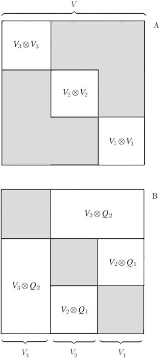 New window|Download| PPT slide