Biqun Chen¹, Karthikeyan Rajagopal^,2, Fatemeh Parastesh³, Hamed Azarnoush³, Sajad Jafari^,3,4, Iqtadar Hussain⁵¹School of Electronic Engineering, Changzhou College of Information Technology, Changzhou 213164, China
²Nonlinear Systems and Applications, Faculty of Electrical and Electronics Engineering, Ton Duc Thang University, Ho Chi Minh City, Vietnam
³Department of Biomedical Engineering, Amirkabir University of Technology, No. 350, Hafez Ave, Valiasr Square, Tehran 159163-4311, Iran
⁴Health Technology Research Institute, Amirkabir University of Technology, No. 350, Hafez Ave, Valiasr Square, Tehran 159163-4311, Iran
⁵Department of Mathematics, Statistics and Physics, Qatar University, Doha 2713, Qatar

Received:2020-03-01Revised:2020-06-29Accepted:2020-06-30Online:2020-10-02


Abstract
The economic and financial systems consist of many nonlinear factors that make them behave as the complex systems. Recently many chaotic finance systems have been proposed to study the complex dynamics of finance as a noticeable problem in economics. In fact, the intricate structure between financial institutions can be obtained by using a network of financial systems. Therefore, in this paper, we consider a ring network of coupled symmetric chaotic finance systems, and investigate its behavior by varying the coupling parameters. The results show that the coupling strength and range have significant effects on the behavior of the coupled systems, and various patterns such as the chimera and multi-chimera states are observed. Furthermore, changing the parameters' values, remarkably influences on the oscillators attractors. When several synchronous clusters are formed, the attractors of the synchronized oscillators are symmetric, but different from the single oscillator attractor.
Keywords： finance system;symmetric attractors;chimera state;synchronization transitions;non-locally coupled network


PDF (2193KB)MetadataMetricsRelated articlesExportEndNote|Ris|BibtexFavorite
Cite this article
Biqun Chen, Karthikeyan Rajagopal, Fatemeh Parastesh, Hamed Azarnoush, Sajad Jafari, Iqtadar Hussain. Observation of chimera patterns in a network of symmetric chaotic finance systems. Communications in Theoretical Physics, 2020, 72(10): 105003- doi:10.1088/1572-9494/aba261

1. Introduction

In 1986 Grandmont and Malgrange [1] discovered the chaotic behavior in economics. After that many nonlinear continuous models have been proposed for explaining the complex economical dynamics, such as the forced van der Pol model [2], the IS-LM model [3] and the Kaldorian model [4]. Financial system has some factors including interest rate, the price of goods, investment demand and stock, which make its behavior nonlinear and complex. Therefore, chaotic behavior can occur in financial systems, especially during the economic crisis [5, 6].

In recent years, methods of statistical physics have been applied successfully and prolifically to study various aspects of social and financial systems [7, 8]. Furthermore, financial systems are well-known to be complex systems [9]. Complex systems which usually consist of large numbers of agents, are time-varying and have interactions in transferring the information. The economic systems are unceasingly influenced by the environment, such as the political system, the stability of the society and international relationships. On the other hand, an economic agent interacts with other agents either in the vicinity like local shops, or distant parties through intermediaries [10]. Motivated by these concepts and after the 2008 crisis, there has been growing attention in using complexity theory notions like tipping points, contagion and networks in financial researches [11].

In this paper, we consider a network of newly presented 3D nonlinear finance chaotic system in order to study the synchronization patterns especially chimera state which has not been studied earlier. Chimera state is a self-organized spatiotemporal pattern displaying coexistence of synchronized and asynchronized regions [12-14]. Starting from the pioneering work of Kuramoto and Battogtokh [15] that discovered this phenomenon in non-locally coupled phase oscillators, the chimera state has attracted many interests in different fields [16-20]. Kapitaniak et al [21] showed chimeras in a network of coupled pendulum like oscillators and also experimentally in mechanical oscillators named Huygens clock. Larger et al [22] reported chimera patterns experimentally in delayed feedback optoelectronic systems. Chimeras have also been investigated in various neuronal networks such as coupled FitzHugh-Nagumo oscillators and HindMarsh-Rose models with different coupling schemes and connection topologies [23-29]. Very recently, Majhi et al [30] presented a comprehensive review of the studies of chimera states in neuronal networks.

For our investigation, we use a finance system which has symmetric coexisting chaotic attractors, as the blocks of the network. The parameters of the coupling are changed and the spatiotemporal patterns and the oscillators' attractors are considered. In the following section, the mathematical model of the system and the coupled network is described. Section 3 presents the results of investigating the effects of coupling strength and coupling range variations on the network pattern and the oscillators' attractors. Finally, the conclusions are given in section 4.

2. Mathematical model

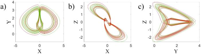
In 2001 Ma and Chen [31] introduced a nonlinear finance chaotic system as:(1)$\begin{eqnarray}\begin{array}{c}\begin{array}{lll}\dot{x} & = & z+\left(y-a\right)x,\\ \dot{y} & = & 1-by-{x}^{2},\\ \dot{z} & = & -x-cz,\end{array}\end{array}\end{eqnarray}$where $x$ represents the interest rate, which is the amount charged, $y$ represents the investment demand, defined as the desired funds and inventories by the organizations, and $z$ represents the price index, which determines the variance of the price distribution. Parameters a, b and c are positive constant parameters and respectively, represent the saving amount, the per-investment cost and the elasticity of demands of commercials. This model has been used by other researchers in different forms [6, 32]. In 2016, Tacha et al [33] modified this model by replacing ${x}^{2}$ term with $\left|x\right|$ in the second equation of the system for better explanation of the real economic world. According to the literature, the interest rate plays a significant role in the investment process and in many countries many banks aim to have small and positive interest rates. The new system was defined as [33]:(2)$\begin{eqnarray}\begin{array}{c}\begin{array}{lll}\dot{x} & = & z+\left(y-a\right)x,\\ \dot{y} & = & 1-by-\left|x\right|,\\ \dot{z} & = & -x-cz.\end{array}\end{array}\end{eqnarray}$

The variables are described as the main system. The new system is rotation symmetric around the y-axis, since it is invariant under the change of coordinates $\left(x,y,z\right)\,\to \,\left(-x,y,-z\right).$ For different values of parameters, the system shows different periodic and chaotic behaviors. Here, we choose the parameters as $a\,=\,1,$ $b\,=\,0.15$ and $c\,=\,1,$ in which the system has chaotic behavior. Figure 1 shows the symmetric coexisting attractors of the system in different planes.

Figure 1.

New window|Download| PPT slide
Figure 1.The symmetric coexisting attractors of the system equation (1) in (a) x-y plane, (b) x-z plane and (c) y-z plane. The initial conditions are $\left(\pm 2,\,1,\,\pm 2\right).$


To construct the network, we couple $N$ numbers of the above systems non-locally by using the nearest neighbor method. It is supposed that the interaction is through the price index variables, so the coupling is made on the z variables. Therefore, the equations of the network can be described as:(3)$\begin{eqnarray}\begin{array}{c}\begin{array}{lll}{\dot{x}}_{i} & = & {z}_{i}+\left({y}_{i}-a\right){x}_{i},\\ {\dot{y}}_{i} & = & 1-b{y}_{i}-\left|{x}_{i}\right|,\\ {\dot{z}}_{i} & = & -{x}_{i}-c{z}_{i}+\displaystyle \frac{d}{2P}\displaystyle \sum _{j=i-P}^{i+P}\left({z}_{j}-{z}_{i}\right),\end{array}\end{array}\end{eqnarray}$where $N$ is the number of systems in the network, $P$ is the number of nearest neighbors in each side and $d$ is the coupling strength.

3. The results

In order to solve the network equations, we use the fourth order Runge-Kutta method with time step $0.01.$ The network size is fixed at $N\,=\,100$ and all the initial conditions are chosen randomly in the interval $x,\,y,\,z\,\in \,\left[-10,\,10\right].$ It should be noted that multiple sets of initial conditions have been considered and the similar results were obtained. The property of coherence and incoherence in the network can be established by using the real-valued local order parameter [34](4)$\begin{eqnarray}{L}_{i}\,=\,\left|\displaystyle \frac{1}{2\delta }\displaystyle {\sum }_{\left|i-k\right|\leqslant \delta }{{\rm{e}}}^{{\rm{j}}{\varnothing }_{k}}\right|,\,i\,=\,1,\ldots ,\,N,\end{eqnarray}$where ${\varnothing }_{k}\,=\,\arctan \left({y}_{k}/{x}_{k}\right)$ denotes the geometric phase of kth unit of the network and j is the imaginary unit (${\rm{j}}\,=\,\sqrt{-1}$). Here, we use the spatial window size of $\delta \,=\,3$ elements. When the local order parameter is smaller than unity, indicates that the kth unit belongs to the incoherent part of the chimera state, and when it is equal to unity, it belongs to coherent parts. To study the network's dynamics completely, firstly, we keep the coupling range constant at $r\,=\,2P/N\,=\,0.4$ and vary the coupling strength and then investigate the effect of changing the coupling range.

3.1. The effect of coupling strength variation

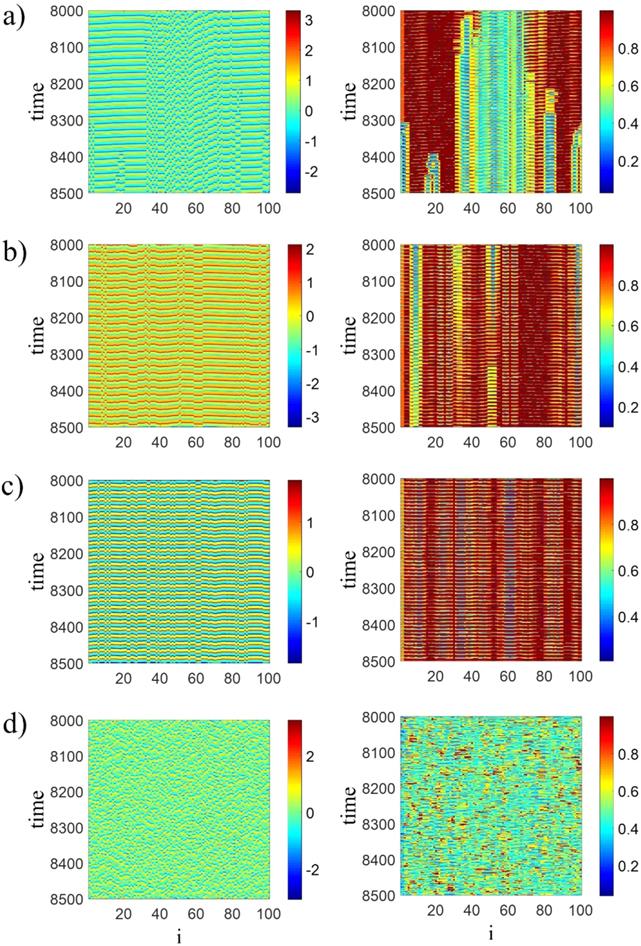
For very small coupling strength with $r\,=\,0.4,$ the network is incoherent. When coupling strength gets higher than $0.005,$ chimera states appear. Figure 2 shows the spatiotemporal patterns and local order parameters for small coupling strengths. By increasing the coupling strength, firstly chimeras are non-stationary and unstable as can be seen in figures 2(a), (b) for $d\,=\,0.006$ and $d\,=\,0.008.$ Then the chimeras become stable, which is shown in figure 2(c) for $d\,=\,0.01.$ But, further increase of coupling strength makes the synchronous clusters to be narrower and thus the network becomes asynchronous at $d\,\gt \,0.02$ (figure 2(d)). For the small values of the coupling strength ($d$), the symmetric coexisting attractors of the single system are not seen any more. In this case, some of the coupled oscillators have one symmetric periodic attractor and some of them have one symmetric chaotic attractor, as shown in figure 3.

Figure 2.

New window|Download| PPT slide
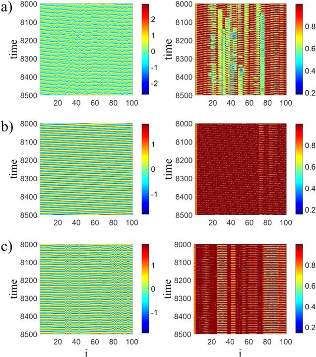
Figure 2.Spatiotemporal patterns (left panel) and local order parameters (right panel) of the network for $r\,=\,0.4,$ (a) non-stationary chimera at $d\,=\,0.006,$ (b) chimera at $d\,=\,0.008,$ (c) chimera at $d\,=\,0.01,$ (d) asynchronization at $d\,=\,0.03.$ The initial conditions are randomly selected in the interval, $y,\,z\,\in \,\left[-10,\,10\right].$ It is observed that for lower coupling strengths, the emerged chimera state is non-stationary, while increasing the coupling strength changes it to stationary one. However, further increasing of $d$ results in asynchronization.

Figure 3.

New window|Download| PPT slide
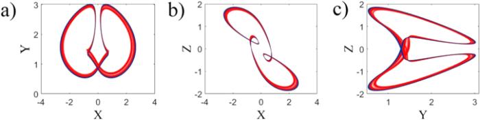
Figure 3.The symmetric attractors of the coupled oscillators (red: chaotic, blue: periodic). (a) x-y plane, (b) x-z plane and (c) y-z plane. The attractors of the coupled oscillators are different from the attractors of single oscillator (shown in figure 1).


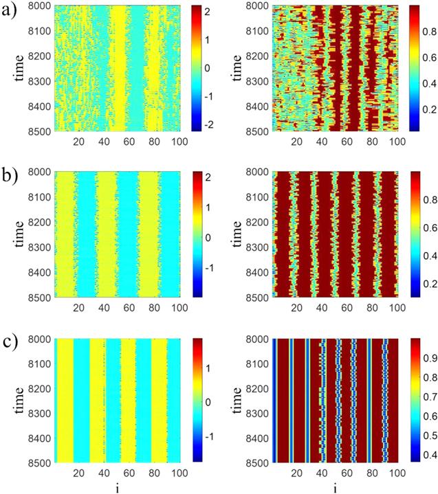
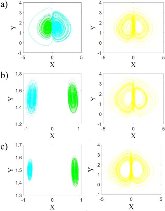
The asynchronous state continues until the coupling strength reaches to $d\,=\,0.77.$ Then the multi-cluster chimeras start to emerge, which seem very regular. Figure 4(a) shows the network pattern for $d\,=\,0.77,$ at which some synchronous regions are formed. In this case, the asynchronous oscillators have the same attractor as the single oscillator (shown in figure 1). While, the oscillators in the synchronous clusters have different attractors. The attractors of the synchronized oscillators (blue and green attractors) and one asynchronous oscillator (yellow attractor) are shown in figure 5. It should be noted that the attractors of the synchronized clusters are symmetric. Figure 4(b) illustrates the pattern of the network for $d\,=\,0.8,$ at which the synchronous region is more than the asynchronous one. In this case, the synchronous clusters have two different symmetric attractors which are shown in figure 5(b) (blue and green attractors). The attractor of the asynchronous oscillators is still similar to the single oscillator (yellow attractor). Raising the coupling strength causes the asynchronous clusters disappear gradually. Figure 4(c) relates to $d\,=\,0.9,$ in which just four solitaries exist and the pattern is imperfect cluster synchronization. Figure 5(c) depicts the attractors of the synchronous systems (blue and green attractors), and the attractor of the solitaries (yellow attractor). As $d$ approaches unity and more than unity, all the systems are attracted with two fixed-points. Figure 6 illustrates the network pattern for $d\,=\,1.2$ in which the systems are attracted by $\left(0.78,\,1.44,\,-0.35\right)$ and $\left(-0.78,\,1.44,\,0.35\right).$

Figure 4.

New window|Download| PPT slide
Figure 4.Spatiotemporal patterns (left panel) and local order parameters (middle panel) of network for $P\,=\,20,$ (a) multi-chimera at $d\,=\,0.77,$ (b) multi-chimera at $d\,=\,0.8,$ (c) imperfect cluster synchronization at $d\,=\,0.9.$ The initial conditions are randomly selected in the interval $x,\,y,\,z\,\in \,\left[-10,\,10\right].$ For larger coupling strengths, multi-chimera states which have multiple synchronized clusters are emerged.

Figure 5.

New window|Download| PPT slide
Figure 5.Attractors of the synchronized oscillators (blue and green) and the asynchronized oscillators (yellow) corresponding to the patterns of figure 6. (a) $d\,=\,0.77,$ (b) $d\,=\,0.8,$ (c) $d\,=\,0.9.$ The attractor of the asynchronized oscillators is the same as the single oscillator, while the synchronized clusters have different symmetric attractors.

Figure 6.

New window|Download| PPT slide
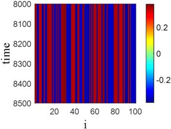
Figure 6.Spatiotemporal pattern of the network for $r\,=\,0.4$ and $d\,=\,1.2.$ For $d\,\gt \,1,$ all of the systems are attracted by two fixed-points (0.78, 1.44, −0.35) and (−0.78, 1.44, 0.35).

3.2. The effect of coupling range variation

Now we investigate the network patterns by changing the nearest neighbor numbers in different coupling strengths, which effects on the patterns significantly. When coupling strength is smaller than $0.2,$ changing the value of $r$ causes multiple transitions between asynchronization, synchronization and chimera states. As an illustration, figure 7 shows network patterns for $d\,=\,0.008$ and different coupling ranges. In this case, when the coupling range is very small, the network is asynchronous as in figure 7(a) for $r\,=\,0.1$ and by increasing $r$ until $r\,=\,0.9,$ chimera states appear as is shown in figure 7(c) for $r\,=\,0.6.$ But in this range, an exception occurs such that for $r$ values near $0.5,$ the oscillators tend to be all synchronized (figure 7(b)). Further increasing of $r$ from $0.9,$ makes the network asynchronous again.

Figure 7.

New window|Download| PPT slide
Figure 7.Spatiotemporal patterns (left panel) and local order parameters (right panel) of network for $d\,=\,0.008,$ (a) asynchronization at $r\,=\,0.1,$ (b) synchronization at $r\,=\,0.5,$ (c) chimera at $r\,=\,0.6.$ The initial conditions are randomly selected in the interval $x,\,y,\,z\,\in \,\left[-10,\,10\right].$ Similar to the coupling strength, the variation of the coupling range can change the network behavior significantly.


The network exhibits asynchronous patterns for $0.2\,\lt \,d\,\lt \,0.7$ for any value of $r.$ In $d\,=\,0.7,$ just for small coupling range, near $r\,=\,0.1,$ chimeras are observed and for more $r$ values, the oscillators oscillate asynchronously. But when $0.7\,\lt \,d\,\lt \,1,$ multi-chimera patterns are observed for most values of $r$ and raising the value of $r$ makes the clusters to be wider. Figure 8 demonstrates this claim for $d\,=\,0.8.$ When $r\,=\,0.1,$ asynchronization occurs in the network as is shown in figure 8(a), but more increase of $r,$ causes multi-chimera states. Comparing figures 8(b) and (c) shows that when more numbers of nearest neighbors are encountered in the coupling, more oscillators are involved in the same clusters. If the coupling range gets more than $0.9,$ the network becomes asynchronous.

Figure 8.

New window|Download| PPT slide
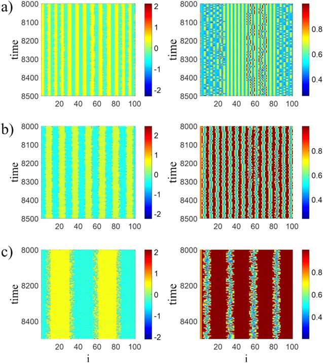
Figure 8.Spatiotemporal patterns (left panel) and local order parameters (right panel) of network for $d\,=\,0.8,$ (a) asynchronization at $r\,=\,0.1,$ (b) multi-chimera at $r\,=\,0.2,$ (c) multi-chimera at $r\,=\,0.6.$ The initial conditions are randomly selected in the interval $x,\,y,\,z\,\in \,\left[-10,\,10\right].$ It is observed that by increasing the coupling range, more oscillators are involved in the clusters and the clusters become wider.


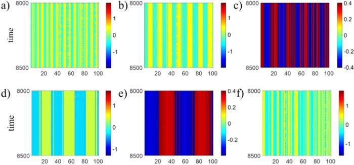
If the coupling strength becomes equal to $1,$ variations of $r$ causes many transitions, and $d\,=\,1$ is a very sensitive point. When $r\,=\,0.1,$ asynchronization is observed and when it approaches to $r\,=\,0.2$ chimeras appear. As $r$ reaches to $0.3,$ all oscillators are attracted by two fixed-points. At $r\,=\,0.4,$ cluster synchronization state appears and in $0.5\,\lt \,r\,\lt \,0.8,$ the attractors change into some near fixed-points. For $r\,=\,0.9,$ the chimera state returns and for global coupling it alters to two fixed-points. The spatiotemporal patterns for all of these cases are shown in figure 9, and their corresponding local order parameters are illustrated in figure 10. If the coupling strength gets higher than unity, the coupling range has no effect and the all the oscillators are attracted by two fixed-points.

Figure 9.

New window|Download| PPT slide
Figure 9.Spatiotemporal patterns of network for $d\,=\,1,$ (a) asynchronization at $r\,=\,0.1,$ (b) chimera at $r\,=\,0.2,$ (c) two fixed-points attractors at $r\,=\,0.3,$ (d) cluster synchronization at $r\,=\,0.4,$ (e) some near fixed-points attractors at $r\,=\,0.7,$ (f) chimera at $r\,=\,0.9.$ The initial conditions are randomly selected in the interval $x,\,y,\,z\,\in \,\left[-10,\,10\right].$ This figure shows at d=1, the value of the coupling range remarkably effects on the network behavior and the oscillators attractors.

Figure 10.

New window|Download| PPT slide
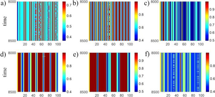
Figure 10.The local order parameters of the states shown in figure 9.

4. Conclusion

In this paper, we investigated a ring network of symmetric finance systems connected via nearest neighbor method. The used finance system is a modification of an old system that can exhibit different symmetric attractors by varying its parameters. Here, to model the real complex behavior of financial networks, we used the parameters in which the system has two symmetric coexisting chaotic attractors. To study the dynamics of the network, the effect of both coupling strength and coupling range variations were considered. It was found that the network shows rich dynamics by changing the coupling parameters, and different behaviors such as asynchronization, synchronization, imperfect cluster synchronizations, chimera and multi-chimera states could be observed. Observing the attractors of the coupled oscillators represented that two different synchronized clusters with symmetric attractors were formed in the network which were different from the single oscillator's attractor. While the attractors of the asynchronized oscillators were similar to the main attractor.

Reference View Option By original order
By published year
By cited within times
By Impact factor

[1]Grandmont J M Malgrange P 1986 J. Econ. Theory 40 3
DOI:10.1016/0022-0531(86)90003-7 [Cited within: 1]

[2]Chian A C L Rempel E L Rogers C 2006 Chaos Solitons Fractals 29 1194
DOI:10.1016/j.chaos.2005.08.218 [Cited within: 1]

[3]De Cesare L Sportelli M 2005 Chaos Solitons Fractals 25 233
DOI:10.1016/j.chaos.2004.11.044 [Cited within: 1]

[4]Lorenz H W 1993 Nonlinear Dynamical Economics and Chaotic Motion Berlin Springer vol 334
[Cited within: 1]

[5]Kocamaz U E Göksu A Taşkın H Uyaroğlu Y 2015 Inf. Technol. Control 44 172
DOI:10.5755/j01.itc.44.2.7732 [Cited within: 1]

[6]Yu H Cai G Li Y 2012 Nonlinear Dyn. 67 2171
DOI:10.1007/s11071-011-0137-9 [Cited within: 2]

[7]Perc M 2019 Sci. Rep. 9 16549
DOI:10.1038/s41598-019-53300-4 [Cited within: 1]

[8]Wang S He S Yousefpour A Jahanshahi H Repnik R Perc M 2020 Chaos Solitons Fractals 131 109521
DOI:10.1016/j.chaos.2019.109521 [Cited within: 1]

[9]Mantegna R N 1999 Eur. Phys. J. B 11 193
DOI:10.1007/s100510050929 [Cited within: 1]

[10]Cilliers P 1998 Complexity and Postmodernism London Routledge
[Cited within: 1]

[11]Battiston S et al. 2016 Science 351 818
DOI:10.1126/science.aad0299 [Cited within: 1]

[12]Bera B K Majhi S Ghosh D Perc M 2017 Europhys. Lett. 118 10001
DOI:10.1209/0295-5075/118/10001 [Cited within: 1]

[13]Dudkowski D Maistrenko Y Kapitaniak T 2016 Chaos 26 116306
DOI:10.1063/1.4967386

[14]Parastesh F Jafari S Azarnoush H Hatef B Bountis A 2018 Chaos Solitons Fractals 110 203
DOI:10.1016/j.chaos.2018.03.025 [Cited within: 1]

[15]Kuramoto Y Battogtokh D 2002 Nonlinear Phenom. Complex Syst. 5 380
[Cited within: 1]

[16]Rakshit S Bera B K Perc M Ghosh D 2017 Sci. Rep. 7 2412
DOI:10.1038/s41598-017-02409-5 [Cited within: 1]

[17]Gjurchinovski A Schöll E Zakharova A 2017 Phys. Rev. E 95 042218
DOI:10.1103/PhysRevE.95.042218

[18]Bogomolov S A Slepnev A V Strelkova G I Schöll E Anishchenko V S 2017 Commun. Nonlinear Sci. Numer. Simul. 43 25
DOI:10.1016/j.cnsns.2016.06.024

[19]Dudkowski D Czołczyński K Kapitaniak T 2019 Nonlinear Dyn. 95 1859
DOI:10.1007/s11071-018-4664-5

[20]Rakshit S Faghani Z Parastesh F Panahi S Jafari S Ghosh D Perc M 2019 Phys. Rev. E 100 012315
DOI:10.1103/PhysRevE.100.012315 [Cited within: 1]

[21]Kapitaniak T Kuzma P Wojewoda J Czolczynski K Maistrenko Y 2014 Sci. Rep. 4 6379
DOI:10.1038/srep06379 [Cited within: 1]

[22]Larger L Penkovsky B Maistrenko Y 2015 Nat. Commun. 6 7752
DOI:10.1038/ncomms8752 [Cited within: 1]

[23]Bera B K Rakshit S Ghosh D Kurths J 2019 Chaos 29 053115
DOI:10.1063/1.5088833 [Cited within: 1]

[24]Majhi S Perc M Ghosh D 2016 Sci. Rep. 6 39033
DOI:10.1038/srep39033

[25]Wei Z Parastesh F Azarnoush H Jafari S Ghosh D Perc M Slavinec M 2018 Europhys. Lett. 123 48003
DOI:10.1209/0295-5075/123/48003

[26]Loos S A Claussen J C Schöll E Zakharova A 2016 Phys. Rev. E 93 012209
DOI:10.1103/PhysRevE.93.012209

[27]Bera B K Ghosh D 2016 Phys. Rev. E 93 052223
DOI:10.1103/PhysRevE.93.052223

[28]Bera B K Ghosh D Lakshmanan M 2016 Phys. Rev. E 93 012205
DOI:10.1103/PhysRevE.93.012205

[29]Majhi S Perc M Ghosh D 2017 Chaos 27 073109
DOI:10.1063/1.4993836 [Cited within: 1]

[30]Majhi S Bera B K Ghosh D Perc M 2019 Phys. Life Rev. 28 100
DOI:10.1016/j.plrev.2018.09.003 [Cited within: 1]

[31]Ma J Chen Y 2001 Appl. Math. Mech. 22 1375
DOI:10.1023/A:1022806003937 [Cited within: 1]

[32]Chen W-C 2008 Chaos Solitons Fractals 36 1305
DOI:10.1016/j.chaos.2006.07.051 [Cited within: 1]

[33]Tacha O Volos C K Kyprianidis I M Stouboulos I N Vaidyanathan S Pham V-T 2016 Appl. Math. Comput. 276 200
DOI:10.1016/j.amc.2015.12.015 [Cited within: 2]

[34]Bera B K Ghosh D Banerjee T 2016 Phys. Rev. E 94 012215
DOI:10.1103/PhysRevE.94.012215 [Cited within: 1]