Na Hao, Yong-Jun Jian^,?School of Mathematical Science, Inner Mongolia University, Hohhot 010021, China

Corresponding authors: ?E-mail:jianyj@imu.edu.cn

Received:2019-06-25Online:2019-10-9

Fund supported:

Supported by the National Natural Science Foundation of China under Grant .No.11772162,11472140 the Natural Science Foundation of Inner Mongolia Autonomous Region of China under Grant .No.2016MS0106 and 2018MS01015 the Inner Mongolia Grassland Talent under Grant .No.12000-12102013 the Research Program of science and technology at Universities of Inner Mongolia Autonomous Region under Grant .No.NJZY18006

Abstract
This paper investigates the magnetohydrodynamic (MHD) electroosmotic flow (EOF) of Newtonian fluid through a zeta potential modulated parallel plate microchannel with patterned hydrodynamic slippage. The driven mechanism of the flow originates from the Lorentz force generated by the interaction of externally imposed lateral electric field $E_y$ and vertical magnetic field $B_z$ and electric field force produced by an externally applied electric field $E_x$. It is assumed that the wall zeta potential and the slip length are periodic functions of axial coordinate $x$, an analytical solution of the stream function is achieved by utilizing the method of separation of variables and perturbation expansion. The pictures of streamlines are plotted and the vortex configurations produced in flow field due to patterned wall potential and hydrodynamic slippage are discussed. Based on the stream function, the velocity field and volume flow rate are obtained, which are greatly depend on some dimensionless parameters, such as slip length $l_s$, electrokinetic width $\lambda$, the amplitude $\delta$ of the patterned slip length, the amplitude $m$ of the modulated zeta potential and Hartmann number $Ha$. The variations of velocity and volume flow rate with these dimensionless parameters are discussed in details. These theoretical results may provide some guidance effectively operating micropump in practical nanofluidic applications.
Keywords： magnetohydrodynamic (MHD) flow;electroosmotic flow (EOF);modulated hydrodynamic slippage;patterned charged surface


PDF (2503KB)MetadataMetricsRelated articlesExportEndNote|Ris|BibtexFavorite
Cite this article
Na Hao, Yong-Jun Jian. Magnetohydrodynamic Electroosmotic Flow with Patterned Charged Surface and Modulated Wettability in a Parallel Plate Microchannel*. [J], 2019, 71(10): 1163-1171 doi:10.1088/0253-6102/71/10/1163

1 Introduction

Nowadays, microfluidic device applications are increasing in the fields of chemical separation, medical diagnostics, material synthesis, energy harvesting, and others.^[1-4] Normally, surface tension, pressure gradient, surface acoustic wave, electric field, magnetic field and their suitable combination have been implemented to manipulate microfluidic flow.^[5-8] Electroosmotic flow (EOF), defined as the motion of fluids in narrow confinements under the action of an axial electric field in the presence of an electric double layer (EDL) near the walls, has wide spectrum of applications.^[9-11] In order to minimize the Joule heating effects in EOF, magnetodydrodynamic (MHD) micropump has been proposed. MHD flow is driven by Lorentz force generated by imposing a lateral electric field and a vertical magnetic field.^[12] Over recent years, many researchers have investigated the MHD flow in microchannel. Rivero and Cuevas^[13] considered the influence of slip condition on the MHD flow in a rectangular microchannel. Jian et al.^[14] analytically studied the transient rotating MHD flow for both DC and AC electric fields through a parallel microchannel. Si and Jian^[15] studied MHD flow of non-Newtonian fluids through two corrugated walls. In order to obtain augmented flow rates, the more general requirement of studying the interaction between EOF and MHD flow is needed. MHD EOF is produced by combining the Lorentz force and electric force in axial direction. Chakraborty and Paul^[16] analyzed the MHD EOF in narrow microchannels and obtained optimized flow rates. Driven by combination of electroosmotic, pressure and magnetic forces, unsteady MHD EOF of incompressible viscous fluid through a circular tube was developed with the Caputo Fabrizio time fractional derivative by Abdulhameed et al. ^[17] Chakraborty et al.^[18] analyzed thermal behavior of MHD EOF in narrow channels taking viscous dissipation and Joule heating into account under constant wall heat flux. Abdulhameed et al.^[19] investigated the MHD EOF flow acted by an arbitrary time-dependent pressure gradient, electric field force and Lorentz force and heat transfer through a cylindrical microchannel. Jian^[20] investigated heat transfer and entropy generation of MHD EOF flow through a slit microchannel. Xie and Jian^[21] studied entropy generation of two-layer MHD EOF flow through microparallel channels. Sarkar et al.^[22] studied heat transfer of MHD EOF with interfacial slip.

Recently, many researchers have investigated the influences of patterned wettability and modulated surface charges on micro-and nanofluidic flows.^[23-24] Hendy et al.^[25] investigated the effect of patterned variations in slip length on micro-and nanofluidic flows. Shit et al.^[26] investigated EOF of non-Newtonian power-law fluid in a micro-channel in the presence of Joule heating effects and examined the effects of thermal radiation and velocity slip conditions. Zhao and Yang^[27] analyzed the EOF of electrolytic solutions in a microchannel with patterned hydrodynamic slippage on channel walls. Pereira^[28] studied the effect of patterned slip on the flow of pressure driven power-law fluids. It was shown that for shear-thickening fluids, patterned slip would induce significant transverse flows comparable in size to those produced for Newtonian fluids. Datta and Choudhary^[29] investigated the EOF through zeta potential patterned nanochannels under slip boundary conditions with constant slip length. Mayur et al.^[30] analyzed the generation of flow vortices in nanoscale confinements under the combined effects of patterned surface charge and substrate wettability. By using molecular dynamics simulations, they theoretically achieved the most efficient microfluidic mixing based upon an optimum patterning frequency for a desired volumetric flow rate. Chaudhury et al.^[31] analyzed the consequences of substrate wettability on the convective heat transfer characteristics in microchannel flows. Ghosh et al.^[32] reported the influence of finite EDL thickness on the EOF over patterned charged surfaces by solving the fully coupled Poisson-Nernst-Planck and Navier-Stokes equations. The effect of imposing shear flow on a charge-modulated EOF was theoretically investigated by Wei.^[33] The flow structures exhibit either saddle points or closed streamlines, depending on the relative strength of an imposed shear to the applied electric field. Ghosh and Chakraborty^[34] focused on evaluating the induced streaming electric field along the orthogonal directions in a narrow fluidic confinement under patterned surface wettability and modulated surface charges. They further demonstrated that the presence of anisotropic modulations on the channel walls gave rise to considerable off-diagonal effects. Ghosh and Chakraborty^[35] studied the alterations of EOF because of interactions between patterned wettability gradients on microfluidic substrates and modulated surface charge distributions. They proved that it is possible to control pattern vortices occurring in the fluidic confinement by using such intricate coupling. Shit and Ranjit^[36] studied effects of different zeta potential and wall slip on MHD EOF through a peristaltically induced micro-channel. They observed that the different zeta potential plays an important role in controlling fluid velocity.

Comparing the above recent studies, we can know that some researchers studied patterned charge surface or modulated wettability on EOF or on MHD, some scholars analyzed both conditions on EOF but no one considers the patterned charge surface and modulated wettability simultaneously on MHD EOF. Therefore, motivated by the concept of multiple field driven microfluidic flow with charge and slip modulated surfaces, the objective of this article is to study the MHD EOF with patterned charged surface and modulated wettability through a parallel plate microchannel. The analytical solutions of stream function, flow velocities and volume flow rates are obtained by using the method of separation of variables and superposition principle. The dependence of velocities and volume flow rates on several nondimensional parameters will be determined graphically. These theoretical results may provide some guidance effectively operating micropump in practical nanofluidic applications.

2 Formulation of the Problem

2.1 Physical Model and Explanation of the Problem

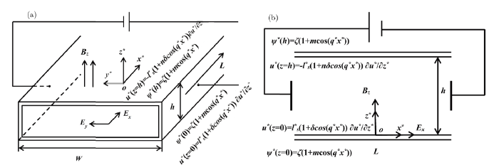
As shown Fig.1(a), we investigate MHD EOF in rectangular microchannels taking patterned surface potential and modulated slip length on walls into consideration. A Cartesian coordinate system $(x^*, y^*, z^*)$ is established with the original point is located at the bottom of channel whose height is $h$, width is W and length is $L$. The upper plate is stipulated at $z=h$ and the lower plate is stipulated at $z=0$. An external electric field $E_x$ is imposed along positive $x^*$-axis, electric field $E_y$ is applied along $y^*$-axis direction and a uniform magnetic field $B_z$ is implemented perpendicular to upper and lower walls of the rectangular channel, i.e., along the positive $z^*$-axis direction. The MHD EOF is driven by the axial Lorentz force generated by the interaction of $E_y$ and $B_z$ and electric field force resulted from $E_x$. Assuming both the height of the channel $h$ and the width $W$ to be much smaller than the length $L$, i.e., $L \gg h$ and $L\gg W$, and the ratio $W/h$ of width to height is very large, so the flow in the rectangular channel can be simplified as the one in two parallel plate microchannels (seen Fig.1(b)). Moreover, patterned zeta potentials on the two walls are the same and can be written as

(1)$$ \psi^*|_{z^*=h}=\psi^*|_{z^*=0}=\zeta[1+m\cos(q^*x^*)]\,, $$
where $\zeta$ is constant wall electrical potential, $m$ is amplitude of the modulated part of the surface potential and $q^*$ is patterned frequency. Furthermore, modulated hydrodynamic slip conditions on the upper and lower walls respectively yield

(2)$$ u^*|_{z^*=h}=-l_s^*[1+n\delta \cos(q^*x^*)]\partial u^*/\partial z^*| _{z^*=h}\,,$$
(3)$$ u^*|_{z^*=0}=l_s^*[1+\delta \cos(q^*x^*)]\partial u^*/\partial z^*| _{z^*=0}\,,$$
where $u^*$ is axial velocity component, $l_s^*$ is constant slip length on walls, $\delta$ is patterned amplitude of the slip length and $n$ is asymmetry factor of patterned interfacial slip. It needs to note that we have assumed the patterned frequencies of zeta potential and slippage on the walls are identical.

New window|Download| PPT slide
Fig. 1Schematic of the physical modeling. (a) 3D view of the MHD EOF micropump and (b) Duct's cross-section of the MHD EOF micropump.

2.2 Electrical Potential Distribution

In the present work, it is notable that the lateral forces (i.e., the Lorentz and electroosmotic forces in $y$-direction) are neglected under the small magnitude of lateral electric field. So the influence of transverse flow weakens, i.e.\ $v\approx0$.^[21] Firstly, considering a symmetric electrolyte solution, the electrical potential $\psi^*$ satisfies Poisson-Boltzmann equation. It is assumed that the electrical potential is much smaller than the thermal potential, i.e. $|\psi^*|\leq k_bT_a/z_ve$, the

Debye -- H$\ddot{\rm u}$ckel approximation $\sinh(z_ve\psi^*/k_bT_a)\approx z_ve\psi^*/k_bT_a$ can be used to simplify the Poisson-Boltzmann equation as^[37-38]

(4)$$ {\bigtriangledown^*}^2\psi^* = {\lambda^*}^2\psi^*\,,$$
where

$$ \bigtriangledown^* = \vec{i}\partial/\partial x^* +\vec{k}\partial/\partial z^*\,,\ \ \lambda^* = (2n_0z_v^2e^2/(\varepsilon k_bT_a))^{(1/2)} $$

is the inverse of the Debye length, $\varepsilon$ is the permittivity of the electrolyte solution, $n_0$ is ion density of bulk solution, $z_v$ is the ion valence, $e$ is the electron charge, $k_b$ is the Boltzmann constant and $T_a$ is the absolute temperature. Introducing the following dimensionless variables

(5)$$ \psi = \psi^*/\zeta\,, \quad x = x^*/h\,,\quad z=z^*/h\,, \lambda=\lambda^*h\,, \quad q=q^*h\,, $$
the dimensionless form of Eq.(4) is

(6)$$ {\bigtriangledown}^2\psi = {\lambda}^2\psi\,, $$
Since Eq.(4) is linear, so the boundary condition(1) can be decompose into constant and modulated zeta potential portions based on the superposition principle. The constant wall zeta potential condition is given by

(7)$$ \psi^*|_{z^*=h} = \zeta\,,\quad \psi^*|_{z^*=0} = \zeta\,,$$
and the modulated zeta potential condition can be written as

(8)$$ ψ*|_{z^*=h} =mζcos(q^*x^*),\ \ \ , ψ^*|_{z^*=0} =mζcos(q^*x^*),. $$
Corresponding dimensionless boundary conditions of Eqs.(7) and (8) are respectively

(9)$$ \psi|_{z=1} = 1\,, \quad \psi|_{z=0} = 1\,,$$
(10)$$ \psi|_{z=1} = m\cos(qx)\,,\quad \psi|_{z=0} = m\cos(qx)\,,$$
By utilizing the method of separation of variables, the solutions of Eq.(6) under the boundary conditions of Eqs.(9) and (10) are given by

(11)$$ \psi = \cosh[\lambda(1/2-z)]/\cosh(\lambda/2)\,, $$
for the constant wall zeta potential condition and

(12)$$ \psi = m\cosh[B(1/2-z)]\cos(qx)/\cosh(B/2)\, $$
for the modulated zeta potential condition, here \(B = (\lambda^2+q^2)^{1/2}\).

2.3 Streaming Function and Flow Fields of the MHD EOF

In present analysis, the flow is two-dimensional due to the patterned zeta potential and modulated wettability. Affected by the magnetic field and electric fields, the momentum and continuity equations of incompressible viscous electrolyte solution can be expressed as^[39]

(13)$$ \rho D\vec{u}^*/Dt^*=-\nabla^*p^*+\mu(\nabla^*)^2\vec{u}^*+\rho_eE_x\vec{i} + \vec{F}\,,$$
(14)$$ \nabla^*\cdot\vec{u}^*=0\,,$$
where $\rho$ is density of the fluid, $\mu$ is dynamic viscosity of the fluid $\vec{u}^*=(\vec{u}^*,0,\vec{w}^*)$ is velocity, $\vec{F}=\vec{J}\times\vec{B}$ is Lorentz force and $\vec{J}=\sigma_e(\vec{E}+\vec{u}^*\times\vec{B})$ is electric current density obtained from Ohm's law.^[40] The expression of electrical conductivity of the electrolyte solution is $\sigma_e = K_{\rm cell}/R$, $K_{\rm cell}$ is conductivity constant, $R$ is resistance. And $\rho_e=-\varepsilon\Delta^*\psi^*$ is charge density. Therefore, the component form of two-dimensional continuity equation and Cauchy momentum equation can be expressed as

(15)$$ \partial u^*/\partial x^*+\partial w^*/\partial z^*=0\,,$$
(16)$$ \mu(\partial^2 u^*/\partial x^{*2}+\partial^2 u^*/\partial z^{*2})-\partial p^*/\partial x^* \quad +\varepsilon\lambda^*\psi^*E_x+\sigma_eB_zE_y-\sigma_eB_z^2u^*=0\,, $$
(17)$$ \mu(\partial^2 w^*/\partial x^{*2}+\partial^2 w^*/\partial z^{*2})-\partial p^*/\partial z^*=0\,.$$
Except for the patterned slip boundary conditions(2) and (3) yielded by axial velocity $u^*$, vertical velocity component $w^*$ of Eqs.(15), (16), and (17) should satisfy the following no-penetration conditions

(18)$$ w^*|_{z^*=0} = 0\,,\quad w^*|_{z^*=h} = 0\,.$$
We would adopt the following non-dimensional variables

(19)$$ w=w^*/u_{eo}\,, \quad u=u^*/u_{eo}\,, \quad p=p^*/p_0\,,\\ l_s=l_s^*/h\,, \quad u_{eo}=-\varepsilon\zeta E_x/\mu\,,\quad p_0=\mu u_{eo}/h\,, S=E_yh\sqrt{\sigma_e/\mu}/u_{eo}\,, \quad Ha=B_zh\sqrt{\sigma_e/\mu}\,,$$
dimensionless governing equations and boundary conditions are rewritten as

(20)$$ \partial u/\partial x+\partial w/\partial z=0\,, $$
(21) $$ \partial^2 u/\partial x^2+\partial^2 u/\partial z^2-\partial p/\partial x+\lambda^2\psi +SHa-Ha^2u=0\,, $$
(22)$$ \partial^2 w/\partial x^2+\partial^2 w/\partial z^2-\partial p/\partial z=0\,, $$
(23)$$ u|_{z=0}=l_s[1+\delta \cos(qx)]\partial u/\partial z| _{z=0}\,, $$
(24)$$ u|_{z=1}=-l_s[1+n\delta \cos(qx)]\partial u/\partial z| _{z=1}\,, $$
(25)$$ w|_{z=0} = 0\,, \quad w|_{z=1} = 0\,,$$
where the parameters $l_s$, $S$ and $Ha$ are non-dimensional slip length, normalized electric field strength in the $y$ direction and Hartmann number respectively. From Eqs.(21) and (22), eliminating the pressure by taking the derivatives of them regarding to $z$ and $x$ respectively, and then subtracting the two derived equations, we have

(26)$$ \partial^3 u/\partial x^2\partial z+\partial^3 u/\partial z^3+\lambda^2\partial\psi/\partial z-Ha^2\partial u/\partial z \\\quad -(\partial^3 w/\partial z^2\partial x+\partial^3 w/\partial x^3)=0\,.$$
Defining a stream function based on Eq.(20)

(27)$$ u=\partial \phi/\partial z, w=-\partial \phi/\partial x\,,$$
Eq.(26) and boundary conditions(23), (24), and (25) can be expressed as

(28)$$ \partial^4\phi /\partial x^4 +2\partial^4 \phi/\partial z^2\partial x^2+\partial^4\phi /\partial z^4 \quad -Ha^2\partial^2\phi/\partial z^2=-\lambda^2\partial\psi/\partial z\,, $$
(29)$$ z|_{z=0}=l_s[1+\delta \cos(qx)]\partial^2 \phi/\partial z^2| _{z=0}\,, $$
(30)$$ z|_{z=1}=-l_s[1+n\delta \cos(qx)]\partial^2 \phi/\partial z^2| _{z=1}\,,$$
(31)$$ \partial\phi/\partial x|_{z=0} = 0\,,\quad \partial\phi/\partial x|_{z=1} = 0\,.$$
Similar to the solving process of electrical potential, the form solution of stream function can be expressed as

(32)$$ \phi=\phi_0+m\phi_1\,,$$
where $\phi_0$ and $m\phi_1$ are the solutions of Eq.(28) when its right hand side term is replaced by the constant and modulated zeta potential solutions(11) and (12). Evidently, Eq.(32) is the stream function while the electrical boundary condition is replaced by the combination of Eqs.(9) and 910). Furthermore, taking the amplitude of the patterned slip length $\delta$ as a small parameter, and $\phi_0$ are $\phi_1$ expanded in the form of power series by using a regular perturbation approach as

(33)$$ \phi_0=\phi_0^0+\delta \phi_0^1+\delta^2 \phi_0^2+O(\delta^3)\,,$$
(34)$$ \phi_1=\phi_1^0+\delta \phi_1^1+\delta^2 \phi_1^2+O(\delta^3)\,.$$
In the following subsections, the solutions of $\phi_0$ and $\phi_1$ will be derived in detail.

(i) Case with constant surface potential and patterned interfacial slip

Substituting Eq.(11) and $\phi_0$ into Eq.(28) yields

(35)$$ \partial^4\phi_0 /\partial x^4 +2\partial^4 \phi_0/\partial z^2\partial x^2+\partial^4\phi_0 /\partial z^4-Ha^2\partial^2\phi_0/\partial z^2 \quad =\lambda^3\sinh[\lambda(1/2-z)]/\cosh(\lambda/2)\,.$$
Inserting the expanded form Eq.(33) of $\phi_0$ into Eq.(35) and related boundary

conditions(29), (30), and (31), then collecting terms of equal powers of $\delta$, governing equations of $\phi_0^0$ , $\phi_0^1$ and $\phi_0^2$ and related boundary conditions can be achieved. In order to describe the process concisely, the details of these problems of each order are ignored. The final results can be written as

(36)$$ \phi_0^0=\lambda\sinh[\lambda(1/2-z)]/[(\lambda^2-Ha^2)\cosh(\lambda/2)] \hphantom{\phi_0^0=} +[l_s\lambda^3\tanh(\lambda/2)+\lambda^2]z/ (\lambda^2-Ha^2)\,,$$
(37)$$ \phi_0^1=f_0(z)\cos(qx)\,,$$
(38)$$ \phi_0^2=f_1(z)\cos(2qx)+c_{22}z+c_{24}\sinh(Haz)\,.$$
The coefficients of $c_{22}$ and $c_{24}$ can be expressed as

(39)$$ c_{24}={l_sf_0^{\prime\prime}(0)+nl_sf_0^{\prime\prime}(1)}{2[Ha-Ha\cosh(Ha)-l_sHa^2\sinh(Ha)]}\,,c_{22}=l_sf_0^{\prime\prime}(0)/2-Hac_{24}\,,$$
and $f_i$ ($i=0,1$) are given in appendix A. Based upon the expression Eq.(33) of stream function, subtracting the values of stream function estimated at $z=1$ and $z=0$ and then eliminating the periodic terms averaged within a period, the volume flow rate is obtained as

(40)$$ Q_0=Q_0^0+\delta^2 Q_0^2+O(\delta^3)\,, $$
(41)$$ Q_0^0=[l_s\lambda^2\tanh(\lambda/2)-2\lambda\tanh(\lambda/2)]/(\lambda^2-Ha^2)\,,$$
(42)$$ Q_0^2=c_{22}+c_{24}\sinh(Ha)\,.$$
(ii)Case with modulated surface potential and patterned interfacial slip

Substituting Eq.(12) and $\phi_1$ into Eq.(28) yields

(43)$$ \partial^4\phi_1 /\partial x^4 +2\partial^4 \phi_1/\partial z^2\partial x^2+\partial^4\phi_1 /\partial z^4-Ha^2\partial^2\phi_1/\partial z^2 \\ \quad =\lambda^2B\sinh[B(1/2-z)]\cos(qx)/\cosh(B/2)\,,$$
Similarly, the expanded terms , $\phi_1^0$, $\phi_1^1$ and $\phi_1^2$ in Eq.(34) of the stream function $\phi_1$ are given by

(44)$$ \phi_1^0=f_2(z)\cos(qx)\,, $$
(45)$$ \phi_1^1=f_3(z)\cos(2qx)+c_{12}z+c_{14}\sinh(Haz)\,,$$
(46)$$ \phi_1^2=f_4(z)\cos(qx)+f_5(z)\cos(3qx)\,.$$
The coefficients of $c_{12}$ and $c_{14}$ are

(47)$$ c_{14}={ l_sf_2^{\prime\prime}(0)+nl_sf_2^{\prime\prime}(1)}{2[Ha-Ha\cosh(Ha)-l_sHa^2\sinh(Ha)]}\,,\\ c_{12}=l_sf_0^{\prime\prime}(0)/2-Hac_{14}\,.$$
$f_i$ ($i=2,3,4,5$) in Eqs.(44), (45), and (46) are also given in Appendix. In the same way, volume flow rate is given by

(48)$$ Q_1=\delta Q_1^1+O(\delta^3)\,,$$
here

(49)$$ Q_1^1=c_{12}+c_{14}\sinh(Ha)\,.$$
Finally, from Eqs.(40) and (48), the whole volume flow rate can be gained as

(50)$$ Q=Q_0^0+\delta^2 Q_0^2+m\delta Q_1^1+O(\delta^3)\,.$$
The flow velocities can be computed by Eq.(27) if stream function is known.

3 Results and Discussion

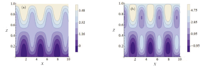
In previous sections, we have obtained the stream function and the velocities of MHD EOF through two patterned charged micro-parallel plates with modulated wettability. The flow strongly depends on some dimensionaless parameters. For typical microfluidic MHD EOF, although Hartmann number $Ha$ should be smaller than $1$ in microfluid, we broaden the range of $Ha$ in order to obtain effect of magnetic field apparently.^[18,41] Besides, the dimensionless slip length changes from $0.01$ to $0.1$,^[35] and the non-dimensional electrokinetic width $\lambda$ means ratio between the height of microchannel and the thickness of electric double layer, is considered from $10$ to $50$^[42-43] although it may be very large in our present problem. The influences of the above mentioned parameters on streamline and flow field are investigated below.

Figures2(a) and 2(b) clearly show the influence of amplitude of the periodic part $m$ on streamlines with other parameters remaining unaltered. At some locations, the vortex occurs with the increase of $m$. The reason why the vortex structure in Fig.2(b) is stronger than that in Fig.2(a) is that the term $m\cos$($qx$) plays a dominant role in boundary conditions.

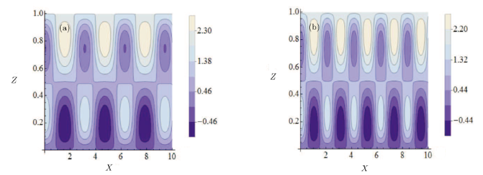
Figure3 demonstrates the variations of streamline with patterned frequency $q$. It is clearly show that the periodicity of the vortex will decrease with an increasing $q$. This result is similar to that obtained in the analysis of EOF.^[35]

New window|Download| PPT slide
Fig.2Streamlines for different $m$ ($l_s=0.05$, $\delta =0.1$, $Ha=3$, $\lambda=50$, $q=2$, $n=2$), (a) $m=5$, (b) $m=12$.

New window|Download| PPT slide
Fig.3Streamlines for different $q$ ($l_s=0.01$, $m=12$, $\delta =0.1$, $Ha=0.5$, $\lambda=50$, $n=3$), (a) $q=2$, (b) $q=3$.



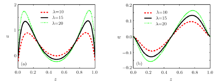
In order to describe the variations of flow field directly, the velocity and the volume flow rate are also discussed in detail. Figure 4 illustrates velocity distribution for different electrokinetic width $\lambda$. It can be observed from Fig.4 that all horizontal velocity components $u$ shows a configuration with M-shape when the slip lengths of two walls is small. At the same time, the vertical velocity component $w$ behaves reverse trends when $z<0.5$ and $z>0.5$ in Fig.4(b), which is an elementary condition to produce vortex. Also, the magnitudes of the velocities $u$ and $w$ become larger with the increase of $\lambda$, especially approaching to the EDL. Mathematically, the reason is that the leading order term in stream function is dominant and is proportional to $\lambda$.

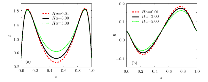
Figure5 depicts the effect of Hartmann number $Ha$ on velocities. From Figs.5(a) and 5(b), it is interesting to note that as $Ha$ gets bigger, the velocities of both directions decreasing monotonously, which demonstrates the $Ha$ acts as an brake to the velocity field. Unlike the trend of velocity in one dimensional flow increase and then decrease as Ha goes up.^[21] The reason is that the influence of aid term $O(HaS)$ within the Lorentz forces in Eq.(21) is eliminated when the flow field is expressed by stream function in Eq.(28).

New window|Download| PPT slide
Fig.4Velocity distributions for different $\lambda$ ($x=2$,$l_s=0.01$, $m=3$, $\delta =0.1$, $Ha=1$, $q=3$, $n=2$), (a) axial velocity $u$; (b) vertical velocity $w$.

New window|Download| PPT slide
Fig.5Velocity distributions for different $Ha$ ($x=2$, $l_s=0.01$, $m=3$, $\delta =0.1$, $q=3$, $\lambda=15$, $n=2$), (a) axial velocity $u$; (b) vertical velocity $w$.



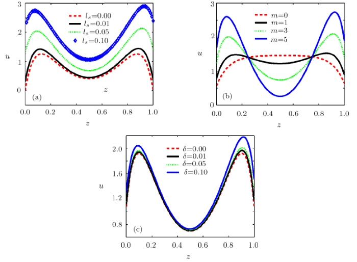
The influence of non-dimensional slip length on velocity distributions is depicted in Fig.6(a). It can be seen from Fig.6(a) that the velocity magnitudes increase with the increase of $l_s$. It is worth noting that $l_s=0$ will lead to no slip condition. The influence of m on the velocity is described in Fig.6(b). The velocity is going to augment with an increasing of $m$. Besides, the minimal value of $m=0$ is associated with the case of uniform zeta potential. The effect of $\delta$ on the velocity is given in Fig.6(c). As is shown, the velocity increases with $\delta$.

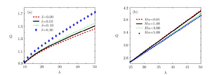
Figure7(a) demonstrates the variations in volume flow rate with electrokinetic width $\lambda$ for four different values of the amplitude of patterned slip length. $\delta = 0$ means the case of constant slip on the walls. For the bigger value of $\delta$, the net flow rate tends to grow. For a prescribed $\delta$, the flow rate increases with $\lambda$ due to the same trend of the velocity. It is observed from Fig.7(b) that an increasing $Ha$ results in a decreasing volume flow rate due to its negative role on the velocity.

New window|Download| PPT slide
Fig.6Velocity distributions for $l_s$, $m$ and $\delta$ ($q=3$, $n=2$), (a) $x=0$, $m=3$, $\delta =0.2$, $\lambda=10$, $Ha=0.5$; (b) $x=2$, $l_s=0.05$, $\delta =0.2$, $\lambda=10$, $Ha=1$; (c) $x=2$, $l_s=0.05$, $m=3$, $\lambda=10$, $Ha=0.5$.

New window|Download| PPT slide
Fig.7Variations of volume flow rates with $\lambda$ for different $\delta$ and $Ha$ ($m=3$, $q=3$), (a) ($l_s=0.01$, $Ha=0.1$, $n=3$); (b) ($l_s=0.05$, $\delta =0.2$, $n=2$).

4 Conclusions

In the present work, we have studied two-dimensional MHD EOF with effects of patterned slip boundary conditions and charge-modulate surfaces through parallel plate microchannels. The analytical solution of stream function has been achieved by using the method of separation of variables and perturbation expansion. Numerical results show that $q$ determines the periodicity of the vortex and $m$ affects the strength of vortex. The velocities of both directions decrease monotonously as $Ha$ becomes larger. This situation is different from one-dimensional MHD EOF where there exists a critical value of the $Ha$. Moreover, the velocities and volume flow rates increase as the increase of the magnitude of patterned zeta potential $m$, modulated amplitude of the slip length $\delta$ and electrokinetic width $\lambda$.

Appendix

(A1)$$ f_0(z)=D_{01}\sinh(\sqrt{y_{11}}z)+D_{02}\cosh(\sqrt{y_{11}}z)+D_{03}\sinh(\sqrt{y_{12}}z)+D_{04}\cosh(\sqrt{y_{12}}z)\,,$$
(A2)$$ f_1(z)=D_{11}\sinh(\sqrt{y_{21}}z)+D_{12}\cosh(\sqrt{y_{21}}z)+D_{13}\sinh(\sqrt{y_{22}}z)+D_{14}\cosh(\sqrt{y_{22}}z)\,,$$
(A3)$$ f_2(z)=D_{21}\sinh(\sqrt{y_{11}}z)+D_{22}\cosh(\sqrt{y_{11}}z)+D_{23}\sinh(\sqrt{y_{12}}z)+D_{24}\cosh(\sqrt{y_{12}}z) {f_2(z)=} +\lambda^2B\sinh[B(1/2-z)]/[(\lambda^4+q^4-2\lambda^2q^2-Ha^2\lambda^2)\cosh(B/2)]\,,$$
(A4)$$ f_3(z)=D_{31}\sinh(\sqrt{y_{21}}z)+D_{32}\cosh(\sqrt{y_{21}}z)+D_{33}\sinh(\sqrt{y_{22}}z)+D_{34}\cosh(\sqrt{y_{22}}z)\,,$$
(A5)$$ f_4(z)=D_{41}\sinh(\sqrt{y_{11}}z)+D_{42}\cosh(\sqrt{y_{11}}z)+D_{43}\sinh(\sqrt{y_{12}}z)+D_{44}\cosh(\sqrt{y_{12}}z)\,,$$
(A6)$$ f_5(z)=D_{51}\sinh(\sqrt{y_{31}}z)+D_{52}\cosh(\sqrt{y_{31}}z)+D_{53}\sinh(\sqrt{y_{32}}z)+D_{54}\cosh(\sqrt{y_{32}}z)\,,$$
(A7)$$ y_{11}=(2q^2+Ha^2+\sqrt{Ha^4+4q^2Ha^2})/2,y_{12}=(2q^2+Ha^2-\sqrt{Ha^4+4q^2Ha^2})/2\,,$$
(A8)$$ y_{21}=(8q^2+Ha^2+\sqrt{Ha^4+16q^2Ha^2})/2,y_{22}=(8q^2+Ha^2-\sqrt{Ha^4+16q^2Ha^2})/2\,,$$
(A9)$$ y_{31}=(18q^2\!+\!Ha^2+\sqrt{Ha^4+36q^2Ha^2})/2,y_{32}=(18q^2+Ha^2-\sqrt{Ha^4+36q^2Ha^2})/2\,,$$
All the coefficients within $f_i$ are obtained by solve the following linear system of equations

(A10)$ \left( \begin{matrix} 0 & 1 & 0 & 1 \\ \\ \sinh(\sqrt{y_{j1}}) & \cosh(\sqrt{y_{j1}}) & \sinh(\sqrt{y_{j2}}) & \cosh(\sqrt{y_{j2}}) \\ \\ \sqrt{y_{j1}} & -l_s\sqrt{y_{j1}} & \sqrt{y_{j2}} & -l_s\sqrt{y_{j2}} \\(\sqrt{y_{j1}}\cosh(\sqrt{y_{j1}}) & (\sqrt{y_{j1}}\sinh(\sqrt{y_{j1}}) & (\sqrt{y_{j2}}\cosh(\sqrt{y_{j2}}) & (\sqrt{y_{j2}}\sinh(\sqrt{y_{j2}}) \\ \\+l_sy_{j1}\sinh(\sqrt{y_{j1}})) & +l_sy_{j1}\cosh(\sqrt{y_{j1}})) & +l_sy_{j2}\sinh(\sqrt{y_{j2}})) & +l_sy_{j2}\cosh(\sqrt{y_{j2}})) \end{matrix} \right)D=X_i\,,$
When $i=0$, $2$, $4$, $j=1$, and when $i=1$, $3$, $j=2$, while $i=5$, $j=3$. $D$ and $X_i$ are expressed as

(A11) $ D=\left( \begin{matrix}D_{i1}\\ D_{i2}\\ D_{i3}\\ D_{i4}\\\end{matrix} \right) ,X_0=\left( \begin{matrix} 0\\ 0\\ l_s\lambda^3\tanh(\lambda/2)/(\lambda^2-Ha^2)\\ nl_s\lambda^3\tanh(\lambda/2)/(\lambda^2-Ha^2)\\ \\ \end{matrix} \right) ,X_1=\left( \begin{matrix} 0\\ 0\\ l_sf_0^{\prime\prime}(0)/2\\ -nl_sf_0^{\prime\prime}(1)/2\\ \end{matrix} \right) ,X_2=\left( \begin{matrix} -\lambda^2B\tanh(B/2)/(\lambda^4+q^4-2\lambda^2q^2-Ha^2\lambda^2)\\\lambda^2B\tanh(B/2)/(\lambda^4+q^4-2\lambda^2q^2-Ha^2\lambda^2)\\(l_s\lambda^2B^3\tanh(B/2)+\lambda^2B^2)/(\lambda^4+q^4-2\lambda^2q^2-Ha^2\lambda^2)\\(l_s\lambda^2B^3\tanh(B/2)+\lambda^2B^2)/(\lambda^4+q^4-2\lambda^2q^2-Ha^2\lambda^2)\\ \end{matrix} \right) , X_3=\left( \begin{matrix} 0\\ 0\\ l_sf_2^{\prime\prime}(0)/2\\ -nl_sf_2^{\prime\prime}(1)/2\\\end{matrix} \right), X_4=\left( \begin{matrix} 0\\ 0\\ l_sf_3^{\prime\prime}(0)/2\\ -nl_s(f_3^{\prime\prime}(1)c_{14}Ha^2\sinh(Ha))/2 \end{matrix} \right), X_5=\left( \begin{matrix} 0\\ 0\\ l_sf_3^{\prime\prime}(0)/2\\ -nl_sf_3^{\prime\prime}(1)/2\\ \end{matrix} \right) $

Reference View Option By original order
By published year
By cited within times
By Impact factor

[1] H. A. Stone, A. D. Stroock, A. Ajdari , Ann. Rev. Fluid Mech. 36(2004) 381.
[Cited within: 1]

[2] C. M. Chang, C. H. Wang, W. H. Chang , et al., Lab on a Chip 13 ( 2013) 1225.


[3] L. Y. Yeo, H. C. Chang, P. P. Y. Chan, J. R. Friend , Small 7(2011) 12.


[4] F. H . Van Der Heyden, D.J. Bonthuis, D. Stein, et al., Nano Lett. 7(2007) 1022.
[Cited within: 1]

[5] S. Ghosl, J. Fluid Mech . 459(2002) 103.
[Cited within: 1]

[6] Y. J. Jian, L. G. Yang, Q. S. Liu , Phys. Fluids. 22(2010) 042001.


[7] M. Buren, Y. J. Jian, L. Chang , J. Phys. D Appl. Phys. 47(2014) 425501.


[8] L. Y. Yeo and J. R. Friend , Ann. Rev. Fluid 46(2014) 379.
[Cited within: 1]

[9] Q. S. Liu, Y. J. Jian, L. G. Yan , Phys. Fluids. 23(2011) 102001.
[Cited within: 1]

[10] Q. S. Liu, Y. J. Jian, L. G. Yang , J. Non-Newtonian Fluid Mech. 166(2011) 478.


[11] Y. Ren, C. Song, W. Liu , et al., Electrophoresis 40 ( 2019) 979.
[Cited within: 1]

[12] J. Jang and S.S. Lee , Sens. Actuator A-Phys. 80(2000) 84.
[Cited within: 1]

[13] M. Rivero and S. Cuevas , Sens. Actuator B-Chem. 166(2012) 884.
[Cited within: 1]

[14] Y. J. Jian, D. Q. Si, L. Chang, Q. S. Liu , Chem. Eng. Sci. 134(2015) 12.
[Cited within: 1]

[15] D. Q . Si and Y. J.Jian, J. Phys. D Appl. Phys. 48(2015) 085501.
[Cited within: 1]

[16] S. Chakraborty and D. Paul , J. Phys. D Appl. Phys. 39(2006) 5364.
[Cited within: 1]

[17] M. Abdulhameed, M. M. Muhammad, A. Y. Gital , et al., Physica A 519 ( 2019) 42.
[Cited within: 1]

[18] R. Chakraborty, R. Dey, S. Chakraborty , Int. J. Heat Mass Transfer 67(2013) 1151.
[Cited within: 2]

[19] M. Abdulhameed, D. Vieru, R. Roslan , Physica A 484(2017) 233.
[Cited within: 1]

[20] Y. J. Jian , Int. J. Heat Mass Transfer 89(2015) 193.
[Cited within: 1]

[21] Z. Y. Xie and Y. J. Jian , Energy 130(2017) 1080.
[Cited within: 3]

[22] S. Sarkar, S. Ganguly, P. Dutta , Int. J. Heat Mass Transfer 100(2016) 451.
[Cited within: 1]

[23] E. Bonaccurso, H. J. Butt, V. S. J . Craig, Phys. Rev. Lett. 90(2003) 144501.
[Cited within: 1]

[24] S. Karakare, A. Kar, A. Kumar, S. Chakraborty , Phys. Rev. E 81(2010) 016324.
[Cited within: 1]

[25] S. C. Hendy, M. Jasperse, J. Burnell , Phys. Rev. E 72(2005) 016303.
[Cited within: 1]

[26] G. C. Shit, A. Mondal, A. Sinha, P. K. Kundu , Physica A. 462(2016) 1040.
[Cited within: 1]

[27] C. Zhao and C. Yang , Electrophoresis 33(2012) 899.
[Cited within: 1]

[28] G. G. Pereira , J. Non-Newton. Fluid 157(2009) 197.
[Cited within: 1]

[29] S. Datta and J. N. Choudhary ,Fluid Dyn. Res . 45(2013) 055502.
[Cited within: 1]

[30] M. Mayur, D. Chakraborty, J. Chakraborty, S. Chakraborty , Phys. Rev. E 85(2012) 016315.
[Cited within: 1]

[31] K. Chaudhury, U. Ghosh, S. Chakraborty , Int. J. Heat Mass Tranfer 67(2013) 1083.
[Cited within: 1]

[32] U. Ghosh, S. Mandal, S. Chakraborty , Phys. Rev. Fluids 2(2017) 064203.
[Cited within: 1]

[33] H. H. Wei, J. Colloid Inter . Sci. 284(2005) 742.
[Cited within: 1]

[34] U. Ghosh and S. Chakraborty , Phys. Rev. E 88(2013) 033001.
[Cited within: 1]

[35] U. Ghosh and S. Chakraborty , Phys. Rev. E 85(2012) 046304.
[Cited within: 3]

[36] G. C. Shit and N. K. Ranjit , Physica A 482(2017) 458.
[Cited within: 1]

[37] Y. P. Liu, Y. J. Jian, Q. S. Liu, F. Q. Li, J. Mol. Liq . 211(2015) 784.
[Cited within: 1]

[38] G. P. Zhao, Y. J. Jian, F. Q. Li, J. Magn. Magn . Mater. 407(2016) 75.
[Cited within: 1]

[39] W. Liu, Y. Ren, F. Chen , et al., Electrophoresis, 40 ( 2019), doi. org/10.1002/elps.201900105.
[Cited within: 1]

[40] S. Moghaddam , Korea-Aust. Rheol. J. 25(2013) 29.
[Cited within: 1]

[41] M. Buren and Y. J. Jian , Electrophoresis 36(2015) 1539.
[Cited within: 1]

[42] L. Chang, Y. J. Jian, M. Buren, Q. S. Liu, Y. J. Sun, J. Mol. Liq . 220(2016) 258.
[Cited within: 1]

[43] Z. Y. Sun, Y. T. Gao, X. Yu, Y. Liu , Colloid Surf. A: Physicochem. Eng. Aspects 366(2010) 1.
[Cited within: 1]