Hydrodynamic Stress Tensor in Inhomogeneous Colloidal Suspensions: an Irving-Kirkwood Extension

删除或更新信息，请邮件至freekaoyan#163.com(#换成@)

本站小编 Free考研考试/2022-01-02

Zong-Li Sun^,¹^,^?, Yan-Shuang Kang^,²^,³^,^?, Yan-Mei Kang⁴1

Science and Technology College, North China Electric Power University, Baoding 071051, China;

College of Science, Hebei Agricultural University, Baoding 071001, China;

College of Chemistry and Environmental Science, Hebei University, Baoding 071001, China;

University of International Relations, Beijing 100091, China

Corresponding authors: ?E-mail:sunzl@ncepu.edu.cn?E-mail:kang_yanshuang@163.com

Received:2019-04-15Online:2019-07-1

Fund supported:

*Supported by the National Natural Science Foundation of China under Grant.No. 21503077
the Fundamental Research Fund for the Central Universities of China under Grant.No. 2016MS156
and the Research Project from Hebei Education Department under Grant.No. QN2018119

Abstract
Based on statistical mechanics for classical fluids, general expressions for hydrodynamic stress in inhomogeneous colloidal suspension are derived on a molecular level. The result is exactly an extension of the Iving-Kirkwood stress for atom fluids to colloidal suspensions where dynamic correlation emerges. It is found that besides the inter-particle distance, the obtained hydrodynamic stress depends closely on the velocity of the colloidal particles in the suspension, which is responsible for the appearance of the solvent-mediated hydrodynamic force. Compared to Brady's stresslets for the bulk stress, our results are applicable to inhomogeneous suspension, where the inhomogeneity and anisotropy of the dynamic correlation should be taken into account. In the near-field regime where the packing fraction of colloidal particles is high, our results can reduce to those of Brady. Therefore, our results are applicable to the suspensions with low, moderate, or even high packing fraction of colloidal particles.
Keywords： hydrodynamic stress;colloidal suspension;diffusion;hydrodynamic force

PDF (223KB)Metadata Metrics Related articlesExportEndNote|Ris|Bibtex Favorite
Cite this article
Zong-Li Sun, Yan-Shuang Kang, Yan-Mei Kang. Hydrodynamic Stress Tensor in Inhomogeneous Colloidal Suspensions: an Irving-Kirkwood Extension ^*. [J], 2019, 71(7): 876-886 doi:10.1088/0253-6102/71/7/876

1 Introduction

In either equilibrium or non-equilibrium of the colloidal suspensions, stress tensor is of supreme importance in the analysis of its static or dynamic properties, including the interfacial tension, transport coefficients, viscoelasticity, and so on.^[1] In their pioneering work, Irving and Kirkwood (IK) derived the stress tensor in atom fluids on a microscopic level.^[2] Though the uniqueness of its representation is still in debate,^[3] it has been extensively employed to describe both static and dynamic aspects of the fluids.^[4-8] In contrast, investigation of the stress in colloidal suspensions is rather primitive. Actually, the stress in colloidal suspension is quite different from that in atom fluids, because of the more complex correlation and multi temporal scales in the suspension. This also makes the investigation on stress in suspension quite tedious.^[9] Nevertheless, due to its close relation to the viscoelastic behavior, stress tensor in colloidal suspension has being a fascinating topic in the studies on its rheological and transport behaviors.

Besides the direct inter-particle correlation, the hydrodynamic interaction (HI) is indispensable in the determination of the stress tensor in the dynamics of suspension. However, it has no counterpart in the equilibrium stress. Intrinsically, the hydrodynamic force on the colloidal particle is nothing but an additional force arising from the flow of solvent, which is caused by the motion of the surrounding particles.^[9-10] In fact, a huge body of researches on the stress tensor in the {bulk} colloidal suspensions have been conducted since the early work of Batchelor et al.,^[11] who introduced firstly the effect of HI on the bulk stress of suspension. Moreover, in the study on the creeping flow on the Smoluchowski time scale, Felderhof has expressed the HI contribution of stress tensor by using of a mobility matrix.^[12] In addition, in the study of the osmotic pressure of a colloidal dispersion, Brady has constructed the HI contribution of the bulk stress by a set of hydrodynamic resistance tensor.^[13-14] Actually, all of these derivations are designed for the bulk suspension. In the confined geometry, however, confinement can dramatically modulate both structural and viscoelastic properties, due either to the interface or to the finite-size effects in the systems.^[15-17] Therefore, in investigations on mass, momentum or energy transport, the inhomogeneity and anisotropy of the stress in the colloidal suspensions should be taken into account.

Actually, in the past decades, dynamics of confined colloidal suspension, especially in the over-damped limit, has attracted considerable attention.^[18-19] By solving Langevin's equations of motion in phase space or the Smoluchowski equation in configurational space, one can achieve the dynamic evolution of the colloidal particles in the suspension.^[20-22] Recently, an even more promising approach, say dynamic density functional theory (DDFT),^[23-27] has been proposed to describe the dynamics of colloidal particles. In most DDFT formalism, the hydrodynamic force is usually described on a two-particle level, such as that proposed by Rotne and Prager.^[28] More importantly, the DDFT contains most of the dynamic information, though some approximation is required in the construction of the DDFT. Therefore, one can resort to DDFT for the structure and motion information of the dynamic suspension, which is indispensable in calculation of the hydrodynamic force and stress.

Though hydrodynamic correlation has achieved satisfactory consideration in DDFT, its contribution to the stress tensor in colloidal suspension is still less satisfactory, especially in the inhomogeneous suspension. Actually, the original IK stress tensor can be extended to the fluid mixture.^[29] However, when the size deference between components is large enough, such simple extension fails to capture all the correlation information in the mixture, because the contribution from hydrodynamic force is not included. In fact, in dense colloidal suspensions, hydrodynamic force may become dominant, and its contribution to the stress becomes important and non-negligible. Therefore, how to take the contribution from hydrodynamic force into account is crucial in the investigation of the colloidal suspensions. In view of this, the hydrodynamic stress in inhomogeneous colloidal suspension will be calculated in this work, and how it relies on the motion of the particles will be discussed.

This paper is organized as follows. In Sec. 2, the IK stress tensor in multi-component fluid mixture is calculated based on the equation of momentum balance. In this section, the IK results are generalized to the colloidal suspension, and the hydrodynamic stress is defined after the determination of the solvent-mediated hydrodynamic forces. In Sec. 3, the velocity of the colloidal particles is determined with the aid of the DDFT, and the hydrodynamic stresses in diffusive suspension, with and without shear flow, are calculated. A comparison of our results with those of Brady's stresslets has also been performed in this section. A discussion on the obtained hydrodynamic stresses is given in Sec. 4.

2 Stress Tensor in Multi-Components Mixtures

Here, we consider a system of colloidal suspension, which is composed of the solvent molecular and colloidal particles. The former of the mass $m_{s}$ and radius $a_{s}$, while the latter of mass $m_{c}$ and radius $a_{c}$. In their dynamic process, they take instantaneous streaming velocities ${{u}}_{s}({{r}},t)$ and ${{u}}_{c}({{r}},t)$, respectively. Firstly, a volume $\mathcal{V}$, with boundary $\mathcal{S}$, is arbitrarily chosen from the suspension. Then, the time rate of change of the total momentum ${{P}}(t)$ in $\mathcal{V}$ can be expressed as:

(1)$$ \frac{d{{P}}}{d t}=\int_{\mathcal{V}} d{{r}} \frac{\partial}{\partial t} \sum_{\nu=s,c}\rho_{\nu}({{r}},t) {{u}}_{\nu}({{r}},t)\,, $$

with $\rho_{\nu}({{r}},t)$ the instantaneous mass density. Actually, there are usually two contributions to the change of the momentum in the volume. One arises from the momentum flow across $\mathcal{S}$, while the other from the action of some force on it. The former can be written as:

(2)$$ \frac{d{{P}}_{1}}{d t}=-\int_{\mathcal{S}} d{{S}} \cdot \sum_{\nu=s,c}\rho_{\nu}({{r}},t) {{u}}_{\nu}({{r}},t) {{u}}_{\nu}({{r}},t)\,, $$

while the latter is given by:

(3)$$ \frac{d{{P}}_{2}}{d t}=\int_{\mathcal{S}} d{{S}} \cdot {\Pi}({{r}},t)\,, $$

with $\boldsymbol{\Pi}$ the stress tensor in the suspension. By utilizing of the Gauss's integral theorem, it is ready to express the momentum continuity equation for the binary mixture as:

(4)$$ \frac{\partial}{\partial t} \sum_{\nu=s,c}\rho_{\nu}({{r}},t) {{u}}_{\nu}({{r}},t) \quad =- \nabla \cdot \Big[ \sum_{\nu=s,c}\rho_{\nu}({{r}},t) {{u}}_{\nu}({{r}},t) {{u}}_{\nu}({{r}},t)-\boldsymbol{\Pi}({{r}},t) \Big]\,. $$

It should be noted that the above equation is applicable for an arbitrary multi-components systems, and that the stress tensor $\boldsymbol{\Pi}({{r}},t)$ should include all the correlations between the components, either static or dynamic correlations.

Actually, Eq. (4) is nothing but the definition of the stress tensor in the suspension, just as its application in the system of simple atom fluid. For the dynamic colloidal suspension under consideration, however, it may become more complex due to the inclusion of dynamic correlations. Even so, it is believed that the stress tensor is still feasible so long as the correlations in the suspension are known. Therefore, in the following, we proceed to express the stress tensor through calculating the time rate of change of the momentum $({\partial}/{\partial t}) \sum_{\nu}\rho_{\nu} {{u}}_{\nu}$.

To take into account the contribution of stress tensor from the thermal motion, it is convenient to separate the laboratory velocity of the $i$-th particle of component $\nu$, into a thermal part ${{v}}_{\nu,i}$ and a streaming part ${{u}}_{\nu}({{r}}_{i},t)$, that is:

(5)$$ \dot{{{r}}}_{\nu,i}={{v}}_{\nu,i} + {{u}}_{\nu}({{r}}_{i},t)\,, $$

with ${{r}}_{\nu,i}$ the position of the particle. Due to the fact that the thermal velocity does not contribute to the momentum current, the time rate of change of the momentum can be rewritten as:

(6)$$ \frac{\partial}{\partial t} \sum_{\nu}\rho_{\nu} {{u}}_{\nu} = \frac{\partial}{\partial t} \sum_{\nu,i} m_{\nu,i} \dot{{{r}}}_{\nu,i} \delta({{r}}-{{r}}_{\nu,i})\,, $$

which can further lead to the following:^[30]

(7)$$ \frac{\partial}{\partial t} \sum_{\nu}\rho_{\nu} {{u}}_{\nu} = -\nabla \cdot \Big[ \sum_{\nu,i} m_{\nu,i} {{v}}_{\nu,i} {{v}}_{\nu,i} \delta({{r}}-{{r}}_{\nu,i}) %\\ + \rho_{\nu} {{u}}_{\nu} {{u}}_{\nu} \Big] + \sum_{\nu,i} {{f}}_{\nu,i} \delta({{r}}-{{r}}_{\nu,i})\,. $$

Comparing with Eq. (4), it is obtained that

(8)$$ \nabla \cdot \boldsymbol{\Pi} = -\nabla \cdot \Big[ \sum_{\nu,i} m_{\nu,i} {{v}}_{\nu,i} {{v}}_{\nu,i} \delta({{r}}-{{r}}_{\nu,i}) \Big] + \sum_{\nu,i} {{f}}_{\nu,i} \delta({{r}}-{{r}}_{\nu,i})\,. $$

Here, ${{f}}_{\nu,i}$ denotes the force exerting on the $i$-th particle of component $\nu$, arising from its interaction with other particles. Accordingly, the second term on the right hand side of Eq. (8) can be rewritten as:

(9)$$ {{f}}_{\nu,i} \delta({{r}}-{{r}}_{\nu,i}) = \frac{1}{2} \sum_{\nu\nu',i\neq j} {{f}}_{\nu\nu',ij} [ \delta({{r}}-{{r}}_{\nu,i}) - \delta({{r}}-{{r}}_{\nu',j}) ]\,. $$

Further, using the fact

$$\delta({{r}}-{{r}}_{i}) - \delta({{r}}-{{r}}_{j})=\nabla \cdot {{r}}_{ij}\int_{0}^{1}d\xi \delta({{r}}-{{r}}_{i} -\xi {{r}}_{ij})\,, $$

and combining Eqs. (8) and (9), it leads to:

(10)$$ \boldsymbol{\Pi}({{r}},t)=-k_{B}T\sum_{\nu} n_{\nu} ({{r}},t){I} + \sum_{\nu\nu'} \boldsymbol{\Pi}_{\nu\nu'}({{r}},t)\,, $$

with ${I}$ the unit tensor. Here, the first term on the right hand side is the kinetic contribution, while the second term denotes the contribution from the intra- and inter-component interactions. In Eq. (10), the stress contribution from the force ${{f}}_{\nu\nu',ij} $ can be given as:

(11)$$ \boldsymbol{\Pi}_{\nu\nu'} = \frac{1}{2} \sum_{i\neq j} {{r}}_{\nu\nu',ij} {{f}}_{\nu\nu',ij} %\\ \int_{0}^{1} \d\xi \delta({{r}}-{{r}}_{\nu,i}-\xi {{r}}_{\nu\nu',ij})\,, $$

with ${{r}}_{\nu\nu',ij} = {{r}}_{\nu' j} - {{r}}_{\nu i}$. Note that the stress contribution in Eq. (11) has been written in the form of summation, which may facilitate its application in the computer simulation. Actually, for the convenience in the theoretical study, one can usually rewrite it, by performing ensemble average, as:

(12)$$ \boldsymbol{\Pi}_{\nu\nu'} = \frac{1}{2} \int d {{r}}_{\nu\nu',ij} {{r}}_{\nu\nu',ij} {{f}}_{\nu\nu',ij} \int_{0}^{1} d \xi n^{(2)}({{r}} - \xi {{r}}_{\nu\nu',ij},{{r}}+(1-\xi){{r}}_{\nu\nu',ij})\,. $$

Some detail about the derivation of Eq. (12) can be found in Appendix A.

Evidently, by substituting the direct inter-particle interaction force ${{f}}_{\nu\nu',ij} \equiv -\nabla \varphi({{r}}_{\nu\nu',ij})$, Eq. (12) is exactly the celebrated IK formula for the potential contribution to the stress. Nevertheless, ${{f}}_{\nu\nu',ij}$ should never be limited to the direct inter-particle forces. It may also arise from the hydrodynamic interaction, because the hydrodynamic force can also impose an additional impact on the change of momentum in the suspension. In view of this, the IK-like formula should also be applicable for the contribution from the hydrodynamic force, which plays the same role as the direct inter-particle force does.

In the colloidal suspension, significant difference between the mass or size of solvent molecular and those of colloidal particle is responsible for the multi temporal scales in the system. Accordingly, on the Brownian time scale, the solvent flow is so fast that the solvent degree-of-freedom can usually be integrated out in the consideration of the motion of colloidal particles.^[9-10] This is the physical interpretation of the hydrodynamic force between colloidal particles. In view of this, the general expression for the stress in colloidal suspension can be written in the following form:

(13)$$ \boldsymbol{\Pi}({{r}},t)=\boldsymbol{\Pi}^{\textrm{kin}}({{r}},t) + \boldsymbol{\Pi}^{\textrm{dir}}({{r}},t) + \boldsymbol{\Pi}^{\textrm{hyd}}({{r}},t)\,. $$

Here, the kinetic contribution

$$ \boldsymbol{\Pi}^{\textrm{kin}}({{r}},t) = -k_{B}T\sum_{\nu} n_{\nu} ({{r}},t){I} $$

is known exactly. Further, by regarding the suspension as a mixture, the contribution from the direct inter-particle interactions can be decomposed into four parts, that is,

$$ \boldsymbol{\Pi}^{\textrm{dir}}({{r}},t) = \boldsymbol{\Pi}_{ss}^{\textrm{dir}}({{r}},t) + \boldsymbol{\Pi}_{sc}^{\textrm{dir}}({{r}},t) + \boldsymbol{\Pi}_{cs}^{\textrm{dir}}({{r}},t) + \boldsymbol{\Pi}_{cc}^{\textrm{dir}}({{r}},t)\,, $$

each of which can be directly obtained by Eq. (12).

It should be noted that $\boldsymbol{\Pi}^{\textrm{dir}}({{r}},t)$ in dynamic suspension should have the same origin as those in the equilibrium phase, because the direct inter-particle forces are independent on the dynamics of the suspension. In contrast, the contribution from HI between colloidal particles, say $\boldsymbol{\Pi}^{\textrm{hyd}}({{r}},t)$, is peculiar in the dynamics, and has no counterpart in the equilibrium stress. Therefore, in the following sections, we focus only on the hydrodynamic stress $\boldsymbol{\Pi}^{\textrm{hyd}}({{r}},t)$. Note also that in the following, the subscripts $\alpha,\beta$ will be used to distinguish the colloidal particles dispersed in suspension.

3 Hydrodynamic Stress in Colloidal Suspension

3.1 Velocity of Colloidal Particles in the Frame-work of DDFT

As mentioned above, significant difference in the temporal scales makes it possible to ignore the dynamical details of the solvent, because the solvent can be regarded as continuum on a Brownian time scale. Besides, the momentum of the particles can also be relaxed to the thermal equilibrium with the heat bath of the solvent. Consequently, the dynamics of the colloidal particles can be described only in the coordinate space by the Smoluchowski equation:^[9]

(14)$$ \frac{\partial}{\partial t}\wp_{c} ({{r}}^{\mathcal{N}_{c}}, t) = \sum_{\alpha\beta} \nabla_{\alpha} \cdot {D}_{\alpha\beta}({{r}}^{\mathcal{N}_{c}}) \cdot \Big[ \frac{1}{k_{B}T} \nabla_{\beta} \Phi({{r}}^{\mathcal{N}_{c}},t) + \nabla_{\beta} \Big] \wp_{c}({{r}}^{\mathcal{N}_{c}},t)\,, $$

with the total number of colloidal particle $\mathcal{N}_{c}$ and the probability distribution function $\wp_{c}({{r}}^{\mathcal{N}_{c}},t)$.In addition, the microscopic diffusion tensor for the colloidal particle can be constructed as:^[31]

(15)$$ {D}_{\alpha\beta}({{r}}^{\mathcal{N}_{c}}) = \delta_{\alpha\beta}{D}^{(0)}({{r}}_{\alpha}) + \delta_{\alpha\beta} \sum_{\gamma\neq\alpha} {D}^{(1)}({{r}}_{\alpha},{{r}}_{\gamma}) + (1-\delta_{\alpha\beta}){D}^{(2)}({{r}}_{\alpha},{{r}}_{\beta})\,, $$

with $\delta_{\alpha\beta}$ the Kronecker delta. The first two terms on the right hand side of Eq. (15) describe the self diffusion, while the remaining describes the collective diffusion. More specifically, ${D}^{(0)}=D_{0}{I}$, with $D_{0}={k_{B}T}/{6\pi\mu a_{c}}$ and the shear viscosity $\mu$, is the self diffusion coefficient in the dilute limit case, in which the hydrodynamic interaction is absent. ${D}^{(1)}({{r}}_{\alpha},{{r}}_{\gamma})=D_{0}[A_{s}(r_{\alpha\beta})\hat{{{r}}}_{\alpha\beta}\hat{{{r}}}_{\alpha\beta} + B_{s}(r_{\alpha\beta})({I}-\hat{{{r}}}_{\alpha\beta}\hat{{{r}}}_{\alpha\beta})]$ represents the effect of its own motion that reflected by the surrounding particles. ${D}^{(2)}({{r}}_{\alpha},{{r}}_{\beta})=D_{0}[A_{c}(r_{\alpha\beta})\hat{{{r}}}_{\alpha\beta}\hat{{{r}}}_{\alpha\beta} + B_{c}(r_{\alpha\beta})({I}-\hat{{{r}}}_{\alpha\beta}\hat{{{r}}}_{\alpha\beta})]$ represents the effect arising from the motion of the other particles. With the method of reflection, one can express:

$$A_{s}(r_{\alpha\beta}) = -\frac{15}{4}\epsilon^{4} + \frac{11}{2}\epsilon^{6} + \mathcal{O}(\epsilon^{8})\,, \\ B_{s}(r_{\alpha\beta}) = -\frac{17}{16}\epsilon^{6} + \mathcal{O}(\epsilon^{8})\,, \\ A_{c}(r_{\alpha\beta}) = \frac{3}{2}\epsilon - \epsilon^{3} + \frac{75}{4}\epsilon^{7} + \mathcal{O}(\epsilon^{9})\,, \\ B_{c}(r_{\alpha\beta}) = \frac{3}{4}\epsilon + \frac{1}{2}\epsilon^{3} + \mathcal{O}(\epsilon^{9})\,, $$

with $\epsilon=a_{c}/r_{\alpha\beta}$ and $\hat{{{r}}}_{\alpha\beta}={{r}}_{\alpha\beta}/r_{\alpha\beta}$.

In Eq. (14), the total potential energy $\Phi({{r}}^{\mathcal{N}_{c}},t)$ in Eq. (14) is given, up to a pairwise level, as:

(16)$$ \Phi({{r}}^{\mathcal{N}_{c}},t) = \sum_{\alpha}V_{\textrm{ext}}({{r}}_{\alpha},t) + \frac{1}{2} \sum_{\alpha\neq\beta} \varphi({{r}}_{\alpha},{{r}}_{\beta})\,, $$

with the external potential $V_{\textrm{ext}}({{r}}_{\alpha},t)$ and the pair potential $\varphi({{r}}_{\alpha},{{r}}_{\beta})$.

On the Brownian time scale, the hydrodynamic force is balanced with the resultant of Brownian and direct inter-particle forces. Accordingly, for the colloidal particle $\alpha$, it reads

(17)$$ {{f}}_{\alpha}^{\textrm{dir}} + {{f}}_{\alpha}^{B} + {{f}}_{\alpha}^{\textrm{{dif}}} =0\,. $$

Here, ${{f}}_{\alpha}^{\textrm{dir}} = -\nabla_{\alpha} \Phi({{r}}_{\alpha\beta})$ is the direct force, while ${{f}}_{\alpha}^{{B}} = -k_{B}T \nabla_{\alpha}\log{\wp_{c}({{r}}^{\mathcal{N}_{c}},t)}$ is the Brownian force.^[9] The total hydrodynamic force ${{f}}_{\alpha}^{\textrm{dif}}$ exerting on the particle $\alpha$ relates to the motion of particles through:

(18)$$ \left (\begin{matrix} {{u}}_{1} \\ \vdots \\ {{u}}_{\mathcal{N}_{c}} \end{matrix} \right ) \!= \! - \frac{1}{k_{B}T} \left (\begin{matrix} {D}_{11} \ \ \cdots \ \ {D}_{1 \mathcal{N}_{c}} \\ \vdots \ \ {D}_{\alpha\beta} \ \ \vdots \\ {D}_{\mathcal{N}_{c}1} \ \ \cdots \ \ {D}_{\mathcal{N}_{c} \mathcal{N}_{c}} \end{matrix} \right ) \left (\begin{matrix} {{f}}_{1}^{\textrm{dif}} \\ \vdots \\ {{f}}_{\mathcal{N}_{c}}^{\textrm{dif}} \end{matrix} \right ). $$

Note that ${{u}}_{\alpha}$ is the diffusion velocity of the particle $\alpha$ with respect to the fixed reference system. This provides us a feasible route to determine the motion of the particles. Combining Eqs.(17) and (18), the diffusion velocity can be given by:

(19)$$ {{u}}_{\alpha} = \frac{1}{k_{B}T} \sum_{\beta} {D}_{\alpha\beta}({{r}}^{\mathcal{N}_{c}}) % \cdot ( {{f}}_{\beta}^{\textrm{dir}} + {{f}}_{\beta}^{{{B}}} )\,. $$

By integrating both sides with $\int d{{r}}^{\mathcal{N}_{c}-1} (\cdot) \wp_{c}({{r}}^{\mathcal{N}_{c}})$, and using the first two members of the Yvon-Born-Green hierarchy,^[32] one obtains the ensemble average of the diffusion velocity, for the particle locating at ${{r}}_{\alpha}$, as:

(20)$$ {{u}}_{\textrm{dif}}({{r}}_{\alpha}) \equiv \langle {{u}}_{\alpha} \rangle = \frac{1}{k_{B}T} \Big[ {D}^{(0)}({{r}}_{\alpha}) \cdot \nabla_{\alpha} \frac{\delta \mathcal{F}[n_{c}]}{\delta n_{c}({{r}}_{\alpha})} \quad + \int d{{r}}_{\beta} n_{c}({{r}}_{\beta}) g_{c}^{(2)}(r_{\alpha\beta}) {D}^{(1)}({{r}}_{\alpha\beta}) \cdot \nabla_{\alpha} \frac{\delta \mathcal{F}[n_{c}]}{\delta n_{c}({{r}}_{\alpha})} \quad + \int d{{r}}_{\beta} n_{c}({{r}}_{\beta}) g_{c}^{(2)}(r_{\alpha\beta}) {D}^{(2)}({{r}}_{\alpha\beta}) \cdot \nabla_{\beta} \frac{\delta \mathcal{F}[n_{c}]}{\delta n_{c}({{r}}_{\beta})} \Big]\,, $$

in which $g_{c}^{(2)}(r_{\alpha\beta})$ is the radial distribution function. Note that in the overdamped limit, the non-equilibrium Helmholtz free energy functional, say $\mathcal{F}[n_{c}]$, can be written in the same form as that of the corresponding equilibrium system, that is,

(21)$$ \mathcal{F}[n_{c}] = k_{B}T \int d {{r}} n_{c}({{r}},t) [\ln(\Lambda^{3} n_{c}({{r}},t))-1] \\ + \mathcal{F}_{\textrm{exc}}[n_{c}] + \int d {{r}} n_{c}({{r}},t) V_{\textrm{ext}}({{r}},t)\,, $$

where $\mathcal{F}_{\textrm{exc}}[n_{c}]$ is the excess free energy functional contributed from the interaction between particles.^[32-33] In Eq. (19), it has been indicated that the determination of $\langle {{u}}_{\alpha} \rangle$ is a complex many-body problem, because the dynamics of each particle relates simultaneously to all the surrounding particles. Fortunately, dynamic density functional theory, which is originally designed to calculate the dynamic evolution of the particle density, provides an effective way to determine the diffusion velocity ${{u}}_{\textrm{dif}}({{r}}_{\alpha})$, just as shown in Eq. (20).

3.2 The Hydrodynamic Stress in Diffusive Suspension

As is known, colloidal suspension is a multi-scaled fluid mixture. On the Brownian time scale, however, the solvent should be regarded as continuum, because the Brownian time scale is long enough for the solvent to relax their momentum and position coordinates to the thermal equilibrium. However, the particle in a viscous solvent can feel the motion of the surrounding particles due to the solvent-mediated hydrodynamic force between them. In contrast to the direct force, the hydrodynamic force is more complex in that it depends not only on the inter-particle distance, but also on the velocity of particles in the suspension. Therefore, in order to determine its contribution to the stress, one should firstly find out the explicit dependence of hydrodynamic force on inter-particle distance and particle velocity.

In the resistance problem of two translating sphere, the total hydrodynamic force ${{f}}_{\alpha}^{\textrm{dif}}$ on particle $\alpha$ can be obtained by using of the method of reflections.^[34] For instance, the result for ${{f}}_{\alpha}^{\textrm{dif}}$, up to the fourth reflection, can be given by:

(22)$$ {{f}}_{\alpha}^{\textrm{dif}} = {{f}}_{\alpha}^{0} \cdot \Big[ 1 + \frac{9}{4}\epsilon^{2}-\frac{117}{16}\epsilon^{4} \Big]\hat{{{r}}}_{\alpha\beta}\hat{{{r}}}_{\alpha\beta} \\ + {{f}}_{\alpha}^{0} \cdot \Big[ 1 + \frac{9}{16}\epsilon^{2}+\frac{63}{256}\epsilon^{4} \Big]({I}-\hat{{{r}}}_{\alpha\beta}\hat{{{r}}}_{\alpha\beta}) \\ + {{f}}_{\beta}^{0} \cdot \Big[ -\frac{3}{2}\epsilon-\frac{19}{8}\epsilon^{3} \Big]\hat{{{r}}}_{\alpha\beta}\hat{{{r}}}_{\alpha\beta} \\ + {{f}}_{\beta}^{0} \cdot \Big[ -\frac{3}{4}\epsilon-\frac{59}{64}\epsilon^{3} \Big]({I}-\hat{{{r}}}_{\alpha\beta}\hat{{{r}}}_{\alpha\beta})\,, $$

with ${{f}}_{\alpha}^{0} = -\gamma {{u}}_{\alpha}$. Note that $\gamma=6\pi\mu a_{c}$ denotes the friction coefficient of an isolated sphere with $\mu$ the shear viscosity. This indicates that for the two-body resistance problem, the hydrodynamic force on particle $\alpha$ has three contributions, which arise respectively from the friction force of the isolated sphere, the reflected field of particle $\alpha$ by particle $\beta$, and the field of particle $\beta$. It is expected that this type of decomposition for ${{f}}_{\alpha}^{\textrm{dif}}$ can be generalized to the many-body resistance problem. In view of this, one can decompose ${{f}}_{\alpha}^{\textrm{dif}}$ into three different types of contribution, that is

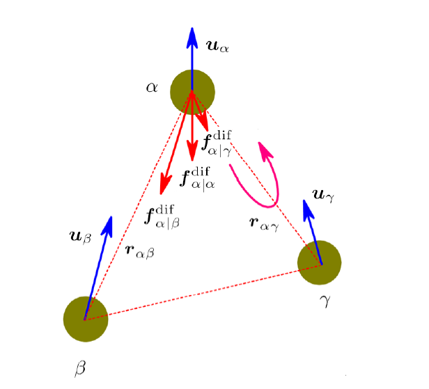
(23)$$ {{f}}_{\alpha}^{\textrm{dif}} = {{f}}_{\alpha|\alpha}^{\textrm{dif}} + \sum_{\gamma\neq\alpha} {{f}}_{\alpha|\gamma}^{\textrm{dif}} + \sum_{\beta\neq\alpha} {{f}}_{\alpha|\beta}^{\textrm{dif}}\,. $$

A sketch for the decomposition of ${{f}}_{\alpha}^{\textrm{dif}}$ is given in Fig. 1. Specifically, in Eq. (23), ${{f}}_{\alpha|\alpha}^{\textrm{dif}}$ denotes the hydrodynamic force of an isolated particle, which can be given as:

(24)$$ {{f}}_{\alpha|\alpha}^{\textrm{dif}} = - \boldsymbol{\Upsilon}^{(0)} \cdot {{u}}_{\textrm{dif}}({{r}}_{\alpha})\,, $$

Fig. 1

New window|Download| PPT slide
Fig. 1(Color online) A sketch for the decomposition of ${f}_{\alpha}^{\textrm{dif}}$, which is exerted on the particle $\alpha$ by the surrounding colloidal particles. In the figure, the blue arrows represent the velocity of particles, while the red arrows stand for different contributions of the solvent-mediated hydrodynamic force. In addition, the pink arrow represents the reflected velocity field by the particle $\gamma$.

with $\boldsymbol{\Upsilon}^{(0)}=\gamma {I}$. As stated above, ${{f}}_{\alpha|\alpha}^{\textrm{dif}}$ is exactly the friction force in a very dilute suspensions, where the hydrodynamic force is absent.

In contrast, ${{f}}_{\alpha|\gamma}^{\textrm{dif}}$ represents the contribution from the $\alpha$-th particle's movement, which is reflected from the particle $\gamma$ and back to the particle $\alpha$. It is given as:

(25)$$ {{f}}_{\alpha|\gamma}^{\textrm{dif}} = - \boldsymbol{\Upsilon}^{(1)}({{r}}_{\alpha\gamma}) \cdot [ {{u}}_{\textrm{dif}}({{r}}_{\alpha}) - {{u}}_{\textrm{dif}}({{r}}_{\gamma}) ]\,, $$

with the resistance tensor $\boldsymbol{\Upsilon}^{(1)}({{r}}_{\alpha\gamma})$. Obviously, ${{f}}_{\alpha|\gamma}^{\textrm{dif}}$ depends not only on the distance between particles $\alpha$ and $\gamma$, but also on the relative velocity between them. In addition, ${{f}}_{\alpha|\beta}^{\textrm{dif}}$ denotes also the hydrodynamic force exerted on the particle $\alpha$ by the solvent, but stems from the motion of the particle $\beta$. This contribution can be given as:

(26)$$ {{f}}_{\alpha|\beta}^{\textrm{dif}} = - \boldsymbol{\Upsilon}^{(2)}({{r}}_{\alpha\beta}) \cdot [ {{u}}_{\textrm{dif}}({{r}}_{\beta}) - {{u}}_{\textrm{dif}}({{r}}_{\alpha}) ]\,, $$

with another resistance tensor $\boldsymbol{\Upsilon}^{(2)}({{r}}_{\alpha\beta})$. Actually, the above-mentioned $\boldsymbol{\Upsilon}^{(0)}$ and $\boldsymbol{\Upsilon}^{(1)}$ are the diagonal elements of the resistance matrix $\boldsymbol{\Upsilon}$, while $\boldsymbol{\Upsilon}^{(2)}$ is the off-diagonal elements of it. Actually, simple expressions for $\boldsymbol{\Upsilon}^{(1)}$ and $\boldsymbol{\Upsilon}^{(2)}$ can be obtained by comparing the results in Eqs. (24)--(26) with those given in Eq. (22), that is,

(27)$$ \boldsymbol{\Upsilon}^{(1)} = \gamma \Big[ \frac{9}{4}\epsilon^{2}-\frac{117}{16}\epsilon^{4} \Big]\hat{{{r}}}_{\alpha\beta}\hat{{{r}}}_{\alpha\beta} \\ + \gamma \Big[ \frac{9}{16}\epsilon^{2}+\frac{63}{256}\epsilon^{4} \Big]({I}-\hat{{{r}}}_{\alpha\beta}\hat{{{r}}}_{\alpha\beta}) \,, \\ \boldsymbol{\Upsilon}^{(2)} = \gamma \Big[ -\frac{3}{2}\epsilon-\frac{19}{8}\epsilon^{3} \Big]\hat{{{r}}}_{\alpha\beta}\hat{{{r}}}_{\alpha\beta} \\ + \gamma \Big[ -\frac{3}{4}\epsilon-\frac{59}{64}\epsilon^{3} \Big]({I}-\hat{{{r}}}_{\alpha\beta}\hat{{{r}}}_{\alpha\beta})\,. $$

Note that in the above, two types of the second-order tensor, say ${D}$ and $\boldsymbol{\Upsilon}$, are used to describe the dynamics of colloidal particles in the suspension. Actually, they describe, respectively, the mobility and resistance problems of the colloidal in the suspension. In general, they are related with each other through $\boldsymbol{\Upsilon}^{-1}={D}/k_{B}T$, which indicates that ${D}$ is the inverse of the entire matrix $\boldsymbol{\Upsilon}$.

According to the decomposition of ${{f}}_{\alpha}^{\textrm{dif}}$ in Eq. (23), the hydrodynamic stress $\boldsymbol{\Pi}^{\textrm{hyd}}$ can also be decomposed into:

(28)$$ \boldsymbol{\Pi}^{\textrm{hyd}}({r}) = \boldsymbol{\Pi}_{\alpha|\alpha}^{\textrm{dif}}({r}) %\\ + \boldsymbol{\Pi}_{\alpha|\gamma}^{\textrm{dif}}({r}) %\\ + \boldsymbol{\Pi}_{\alpha|\beta}^{\textrm{dif}}({r})\,. $$

Substituting Eqs. (25) and (26) into Eq. (12), one obtains the last two terms, respectively, as:

(29)$$ \boldsymbol{\Pi}_{\alpha|\gamma}^{\textrm{dif}}({r}) = - \frac{1}{2} \int d {{r}}_{\alpha\gamma} {{r}}_{\alpha\gamma}\boldsymbol{\Upsilon}^{(1)}({{r}}_{\alpha\gamma}) \\ \hphantom{\boldsymbol{\Pi}_{\alpha|\gamma}^{\textrm{dif}}({r}) =} \cdot [ {{u}}_{\textrm{dif}}({{r}}_{\alpha}) - {{u}}_{\textrm{dif}}({{r}}_{\gamma}) ] \hphantom{\boldsymbol{\Pi}_{\alpha|\gamma}^{\textrm{dif}}({r}) =} \\ \times \int_{0}^{1} d \xi n_{c}^{(2)}({{r}} - \xi {{r}}_{\alpha\gamma},{{r}}+(1-\xi){{r}}_{\alpha\gamma})\,, $$

(30)$$ \boldsymbol{\Pi}_{\alpha|\beta}^{\textrm{dif}}({r}) = - \frac{1}{2} \int d {{r}}_{\alpha\beta} {{r}}_{\alpha\beta}\boldsymbol{\Upsilon}^{(2)}({{r}}_{\alpha\beta}) \\ \hphantom{\boldsymbol{\Pi}_{\alpha|\gamma}^{\textrm{dif}}({r}) =} \cdot [ {{u}}_{\textrm{dif}}({{r}}_{\beta}) - {{u}}_{\textrm{dif}}({{r}}_{\alpha}) ] \hphantom{\boldsymbol{\Pi}_{\alpha|\gamma}^{\textrm{dif}}({r}) =} \\ \times \int_{0}^{1} d \xi n_{c}^{(2)}({{r}} - \xi {{r}}_{\alpha\beta},{{r}}+(1-\xi){{r}}_{\alpha\beta})\,. $$

Note that in the above equations, ${{f}}_{\alpha|\gamma}^{\textrm{dif}}$ and ${{f}}_{\alpha|\beta}^{\textrm{dif}}$ have been regarded as pairwise forces, which are mediated by the solvent.

From above, it is obvious that ${{f}}_{\alpha|\gamma}^{\textrm{dif}}$ and ${{f}}_{\alpha|\beta}^{\textrm{dif}}$ depend closely on the velocity of other particles. In contrast, the friction force ${{f}}_{\alpha|\alpha}^{\textrm{dif}}$ relates only to the motion of its own. Therefore, the friction force can be treated as a thermodynamic force, whose contribution to the stress tensor can be given by:

(31)$$ \boldsymbol{\Pi}_{\alpha|\alpha}^{\textrm{dif}} = - \frac{1}{\mathcal{V}} \sum_{\alpha} {{r}}_{\alpha} {{f}}_{\alpha|\alpha}^{\textrm{dif}}\,. $$

Inserting the expression for ${{f}}_{\alpha|\alpha}^{\textrm{dif}}$ and performing ensemble average, $\boldsymbol{\Pi}_{\alpha|\alpha}^{\textrm{dif}}$ can be rewritten as:

(32)$$ \boldsymbol{\Pi}_{\alpha|\alpha}^{\textrm{dif}}({r}) = n_{c}({r}) {r} \boldsymbol{\Upsilon}^{(0)}({r}) \cdot {{u}}_{\textrm{dif}}({r})\,. $$

Some details about the derivation of Eq. (32) can be found in Appendix B. Collecting the results in Eqs. (29), (30), and (32), one obtains the hydrodynamic stress contribution from the interaction ${{f}}_{\alpha}^{\textrm{dif}}$, as:

(33)$$ \boldsymbol{\Pi}^{\textrm{hyd}}({{r}}) = n_{c}({{r}}) {{r}} \boldsymbol{\Upsilon}^{(0)}({{r}}) \cdot {{u}}_{\textrm{dif}}({{r}}) \hphantom{\boldsymbol{\Pi}^{\textrm{hyd}}({{r}}) =} \\ - \frac{1}{2} \int d {{r}}_{\alpha\gamma} {{r}}_{\alpha\gamma}\boldsymbol{\Upsilon}^{(1)}({{r}}_{\alpha\gamma}) \\ \hphantom{\boldsymbol{\Pi}^{\textrm{hyd}}({{r}}) =} \cdot [ {{u}}_{\textrm{dif}}({{r}}_{\alpha}) - {{u}}_{\textrm{dif}}({{r}}_{\gamma}) ] \hphantom{\boldsymbol{\Pi}^{\textrm{hyd}}({{r}}) =} \\ \times \int_{0}^{1} d \xi n_{c}^{(2)}({{r}} - \xi {{r}}_{\alpha\gamma},{{r}}+(1-\xi){{r}}_{\alpha\gamma}) \hphantom{\boldsymbol{\Pi}^{\textrm{hyd}}({{r}}) =} \\ - \frac{1}{2} \int d {{r}}_{\alpha\beta} {{r}}_{\alpha\beta}\boldsymbol{\Upsilon}^{(2)}({{r}}_{\alpha\beta}) \\ \hphantom{\boldsymbol{\Pi}^{\textrm{hyd}}({{r}}) =} \cdot [ {{u}}_{\textrm{dif}}({{r}}_{\beta}) - {{u}}_{\textrm{dif}}({{r}}_{\alpha}) ] \hphantom{\boldsymbol{\Pi}^{\textrm{hyd}}({{r}}) =} \\ \times \int_{0}^{1} d \xi n_{c}^{(2)}({{r}} - \xi {{r}}_{\alpha\beta},{{r}}+(1-\xi){{r}}_{\alpha\beta})\,. $$

Note that Eq. (33) gives the stress contribution from the hydrodynamic force in a diffusive suspension, where the solvent has been considered as a continuum. Further, in the dilute limit, there is no hydrodynamic interaction. In this situation, the last two terms in Eq. (33) disappear, and only the first term remains.

In practice, at any moment of a dynamic process, the involved pair density of the fluid can be further expressed as: $n_{c}^{(2)}({{r}}_{\alpha},{{r}}_{\beta})=n_{c}({{r}}_{\alpha})n_{c}({{r}}_{\beta})g(r_{\alpha\beta})$, with $g(r_{\alpha\beta})$ the pair distribution function. In the framework of DDFT, this is also a requirement to close the non-linear equation for the one-particle distribution.^[18,24] Actually, $g(r_{\alpha\beta})$ in non-equilibrium fluid can usually be approximated by that of an equilibrium fluid with the same one body density profile, which has been proven to be effective in investigations on non-equilibrium properties of diverse fluids.[18-19,23-25,27,29]

3.3 Hydrodynamic Stress in Suspension with a Shear Flow

In the above, we have focused on the hydrodynamic stress tensor in a diffusive colloidal suspension, particularly on that arising from the inter-particle hydrodynamic force. When the suspension is subjected to a shear flow, the involved hydrodynamic interaction may become even more complex because of the non-uniform flow velocity, say ${E}\cdot {{r}}$, in the solvent. Here, ${E} =({1}/{2})[\nabla {{v}} + (\nabla {{v}})^{\rm T}]$ is the symmetrical part of the rate of strain tensor of the solvent, and ${{v}}$ denotes the velocity field of the solvent. In addition, the flow around each particle can be distorted by the presence of the other particles, which leads to the flow disturbance. Accordingly, the hydrodynamic force on the particle $\alpha$ can be expressed as

(34)$$ {{f}}_{\alpha}^{\textrm{sf}} = -\sum_{\beta} \boldsymbol{\Upsilon}_{\alpha\beta} \cdot [ {{u}}_{\beta} - {E} \cdot {{r}}_{\beta} ] + {C}_{\alpha}:{E}\,, $$

with ${C}_{\alpha}$ the disturbance tensor of rank three, and ${{u}}_{\beta}$ the velocity of colloidal particle $\beta$ in the shear flow. Here, the term ${C}_{\alpha}:{E}$ stands for the involved hydrodynamic force arising from the disturbance in the solvent.

On the Brownian time scale, the above hydrodynamic force on a given particle is balanced by other forces exerting on it, that is

(35)$$ -\sum_{\beta} \boldsymbol{\Upsilon}_{\alpha\beta} \cdot [ {{u}}_{\beta} - {E} \cdot {{r}}_{\beta} ] + {C}_{\alpha}:{E} - \nabla_{\alpha} \Phi({{r}}^{\mathcal{N}_{c}}) \\ \quad - k_{B}T \nabla_{\alpha} \log{\wp_{c}({{r}}^{\mathcal{N}_{c}},t)} =0\,. $$

Accordingly, the relative velocity of the particle $\alpha$ with respect to the shear flow, defined as ${{u}}_{\alpha}^{\textrm{rel}}={{u}}_{\alpha}-{E} \cdot {{r}}_{\alpha}$, can be given by:

(36)$$ {{u}}_{\alpha}^{\textrm{rel}} = {{u}}_{\alpha}^{\textrm{rel-1}} + {{u}}_{\alpha}^{\textrm{rel-2}}\,, $$

with

(37)$$ {{u}}_{\alpha}^{\textrm{rel-1}} = \frac{1}{k_{B}T} \sum_{\beta} \boldsymbol{\Upsilon}^{-1}_{\alpha\beta}({{r}}^{\mathcal{N}_{c}}) \\ \cdot [ -\nabla_{\beta} \Phi({{r}}^{\mathcal{N}_{c}},t) - k_{B}T \nabla_{\beta} \log{\wp_{c}({{r}}^{\mathcal{N}_{c}},t)} ]\,, \\ {{u}}_{\alpha}^{\textrm{rel-2}} = \frac{1}{k_{B}T} \sum_{\beta\neq\alpha} \boldsymbol{\Upsilon}^{-1}_{\alpha\beta} \cdot {C}_{\beta}:{E}\,. $$

In Eq. (36), it is obvious that ${{u}}_{\alpha}^{\textrm{rel}}$ has two contributions, which arise respectively from the sum of inter-particle and Brownian interactions, and the disturbance in the solvent. Further, one can calculate their ensemble averages to obtain local values of ${{u}}_{\alpha}^{\textrm{rel-1}}$ and ${{u}}_{\alpha}^{\textrm{rel-2}}$, that is, ${{u}}_{\textrm{rel-1}}({{r}}_{\alpha})=\langle {{u}}_{\alpha}^{\textrm{rel-1}} \rangle$ and ${{u}}_{\textrm{rel-2}}({{r}}_{\alpha})=\langle {{u}}_{\alpha}^{\textrm{rel-2}} \rangle$. Accordingly, the local relative velocity of particle at ${{r}}_{\alpha}$ can be determined by:

(38)$$ {{u}}_{\textrm{rel}}({{r}}_{\alpha}) = {{u}}_{\textrm{rel-1}}({{r}}_{\alpha}) + {{u}}_{\textrm{rel-2}}({{r}}_{\alpha})\,. $$

Actually, ${{u}}_{\textrm{rel-1}}({{r}}_{\alpha})$ is exactly the result given in Eq. (20), but the involved $n_{c}({r})$ should be the particle density for the suspension with a shear flow.

Similar to the case of diffusion without shear flow, the hydrodynamic force of particle $\alpha$ in suspension with a shear flow can also be decomposed into three contributions, which arise respectively from the relative motion of particle $\alpha$ with respect to solvent, the reflected motion of particle $\alpha$ by the surrounding particles, and the motion of other particles. That is,

(39)$$ {{f}}_{\alpha}^{\textrm{sf}} = {{f}}_{\alpha|\alpha}^{\textrm{sf}} + \sum_{\gamma\neq\alpha} {{f}}_{\alpha|\gamma}^{\textrm{sf}} + \sum_{\beta\neq\alpha} {{f}}_{\alpha|\beta}^{\textrm{sf}}\,. $$

On the other hand, both ${{u}}_{\textrm{rel-1}}({{r}}_{\alpha})$ and ${{u}}_{\textrm{rel-2}}({{r}}_{\alpha})$ contribute to the stress in the suspension. Consequently, one can denote their contributions to the stress as $\boldsymbol{\Pi}^{\textrm{sf-1}}$ and $\boldsymbol{\Pi}^{\textrm{sf-2}}$, respectively. After a similar calculation as performing in the previous section, one can obtain $\boldsymbol{\Pi}^{\textrm{sf-1}}({{r}})$ as:

(40)$$ \boldsymbol{\Pi}^{\textrm{sf-1}}({{r}}) = n_{c}({{r}}) {{r}} \boldsymbol{\Upsilon}^{(0)}({{r}}) \cdot {{u}}_{\textrm{rel-1}}({{r}}) \hphantom{\boldsymbol{\Pi}^{\textrm{sf-1}}({{r}}) =} \\ - \frac{1}{2} \int d {{r}}_{\alpha\gamma} {{r}}_{\alpha\gamma}\boldsymbol{\Upsilon}^{(1)}({{r}}_{\alpha\gamma}) \\ \hphantom{\boldsymbol{\Pi}^{\textrm{sf-1}}({{r}}) =} \cdot [ {{u}}_{\textrm{rel-1}}({{r}}_{\alpha}) - {{u}}_{\textrm{rel-1}}({{r}}_{\gamma}) ] \hphantom{\boldsymbol{\Pi}^{\textrm{sf-1}}({{r}}) =} \\ \times \int_{0}^{1} d \xi n_{c}^{(2)}({{r}} - \xi {{r}}_{\alpha\gamma},{{r}}+(1-\xi){{r}}_{\alpha\gamma}) \hphantom{\boldsymbol{\Pi}^{\textrm{sf-1}}({{r}}) =} \\ - \frac{1}{2} \int d {{r}}_{\alpha\beta} {{r}}_{\alpha\beta}\boldsymbol{\Upsilon}^{(2)}({{r}}_{\alpha\beta}) \\ \hphantom{\boldsymbol{\Pi}^{\textrm{sf-1}}({{r}}) =} \cdot [ {{u}}_{\textrm{rel-1}}({{r}}_{\beta}) - {{u}}_{\textrm{rel-1}}({{r}}_{\alpha}) ] \hphantom{\boldsymbol{\Pi}^{\textrm{sf-1}}({{r}}) =} \\ \times \int_{0}^{1} d \xi n_{c}^{(2)}({{r}} - \xi {{r}}_{\alpha\beta},{{r}}+(1-\xi){{r}}_{\alpha\beta})\,. $$

Comparing with the case without shear flow, it is obvious that this equation can be rewritten as

(41)$$ \boldsymbol{\Pi}^{\textrm{sf-1}}({{r}}) = \boldsymbol{\Pi}_{\alpha|\alpha}^{\textrm{dif}}({{r}})+\boldsymbol{\Pi}_{\alpha|\gamma}^{\textrm{dif}}({{r}})+\boldsymbol{\Pi}_{\alpha|\beta}^{\textrm{dif}}({{r}}) \,, $$

which suggests that $\boldsymbol{\Pi}^{\textrm{sf-1}}({{r}})$ is nothing but the diffusion term of the hydrodynamic stress. Following a similar treatment, the stress contribution from ${{u}}_{\textrm{rel-2}}({{r}})$ can be obtained as:

(42)$$ \boldsymbol{\Pi}^{\textrm{sf-2}}({{r}}) = n_{c}({{r}}) {{r}} \boldsymbol{\Upsilon}^{(0)}({{r}}) \cdot {{u}}_{\textrm{rel-2}}({{r}}) \hphantom{\boldsymbol{\Pi}^{\textrm{sf-2}}({{r}}) =} \\ - \frac{1}{2} \int d {{r}}_{\alpha\gamma} {{r}}_{\alpha\gamma}\boldsymbol{\Upsilon}^{(1)}({{r}}_{\alpha\gamma}) \\ \hphantom{\boldsymbol{\Pi}^{\textrm{sf-2}}({{r}}) =} \cdot [ {{u}}_{\textrm{rel-2}}({{r}}_{\alpha}) - {{u}}_{\textrm{rel-2}}({{r}}_{\gamma})] \hphantom{\boldsymbol{\Pi}^{\textrm{sf-2}}({{r}}) =} \\ \times \int_{0}^{1} d \xi n_{c}^{(2)}({{r}} - \xi {{r}}_{\alpha\gamma},{{r}}+(1-\xi){{r}}_{\alpha\gamma}) \hphantom{\boldsymbol{\Pi}^{\textrm{sf-2}}({{r}}) =} \\ - \frac{1}{2} \int d {{r}}_{\alpha\beta} {{r}}_{\alpha\beta}\boldsymbol{\Upsilon}^{(2)}({{r}}_{\alpha\beta}) \\ \hphantom{\boldsymbol{\Pi}^{\textrm{sf-2}}({{r}}) =} \cdot [ {{u}}_{\textrm{rel-2}}({{r}}_{\beta}) - {{u}}_{\textrm{rel-2}}({{r}}_{\alpha}) ] \hphantom{\boldsymbol{\Pi}^{\textrm{sf-2}}({{r}}) =} \\ \times \int_{0}^{1} d \xi n_{c}^{(2)}({{r}} - \xi {{r}}_{\alpha\beta},{{r}}+(1-\xi){{r}}_{\alpha\beta})\,. $$

In contrast to $\boldsymbol{\Pi}^{\textrm{sf-1}}({{r}})$, $\boldsymbol{\Pi}^{\textrm{sf-2}}({{r}})$ is a disturbance term in the hydrodynamic stress. The results in $\boldsymbol{\Pi}^{\textrm{sf-2}}({{r}})$ indicate that the presence of shear flow has complicated the expression of the hydrodynamic stress, through the effect of the flow disturbance embedded in ${{u}}_{\textrm{rel-2}}({{r}})$.

However, this is not the whole. In the above calculation for the hydrodynamic stress, we have taken only into account the relative velocity of particle with respect to the flowing solvent. In fact, even in the dilute limit, the shear flow itself should contribute to the stress in the suspension, which can be given, on the one-particle level, as:

(43)$$ \boldsymbol{\Pi}^{{E}}({{r}}) = n_{c}({{r}}_{\alpha}) {R}_{\text{SE}} : {E}\,. $$

Here, ${R}_{\rm SE}$ is a rank-four tensor, and its magnitude is known as $|{R}_{\rm SE}|=({20}/{3})\pi\mu a_{c}^{3}$.^[10] By summing $\boldsymbol{\Pi}^{\textrm{sf-1}}({{r}})$, $\boldsymbol{\Pi}^{\textrm{sf-2}}({{r}})$, and $\boldsymbol{\Pi}^{{E}}({{r}})$, one can finally express the hydrodynamic stress in a shear flow, as:

(44)$$ \boldsymbol{\Pi}^{\textrm{hyd}}({{r}}) = \boldsymbol{\Pi}^{\textrm{sf-1}}({{r}}) + \boldsymbol{\Pi}^{\textrm{sf-2}}({{r}}) + \boldsymbol{\Pi}^{{E}}({{r}})\,. $$

3.4 Comparison with Brady's Stresslets in a Shear Flow

In suspension mechanics, the concept of stresslet has been a useful tool for understanding the rheology of suspension and its mixture. It is the symmetric portion of the first moment of the force distribution in suspension. Though the stresslet is unnecessary in the equations of motion for a particle, it is an important bridge between the force distribution and the motion of the suspension. By introducing a set of hydrodynamic resistance tensor, Brady had proposed the expressions for the bulk stress in a suspension with shear flow:^[13-14]

(45)$$ \boldsymbol{\Pi}_{\textrm{Brady}}^{\textrm{hyd}} = n_{c} [\langle {S}^{H} \rangle + \langle {S}^{P} \rangle + \langle {S}^{B} \rangle ]\,, $$

with

(46)$$ \langle {S}^{H} \rangle = - \langle {R}_{\rm SU} \cdot {R}_{\rm FU}^{-1} \cdot {R}_{\rm FE} - {R}_{\rm SE} \rangle : \langle {E} \rangle \,, \\ \langle {S}^{P} \rangle = - \langle {R}_{\rm SU} \cdot {R}_{\rm FU}^{-1} \cdot {{f}}^{\textrm{dir}}\rangle \,, \\ \langle {S}^{B} \rangle = - \langle {R}_{\rm SU} \cdot {R}_{\rm FU}^{-1} \cdot {{f}}^{{B}}\rangle\,. $$

The hydrodynamic stresslet $\langle {S}^{H} \rangle$ is a moment of the fluid traction force taken over the surface of a particle. Therefore, it represents the average of the continuum stress inside that particle. The inter-particle stresslet $\langle {S}^{P} \rangle$ arises from the solvent-mediated hydrodynamic forces, while the Brownian stresslet $\langle {S}^{B} \rangle$ stems from the thermal fluctuations of the solvent. Actually, Brady's result has obtained wide usage in the investigation of viscoelasticity in suspensions.^[35-38] Therefore, in the following, we will compare our results with Eq. (45) to show that our derivation includes all the contributions that presented in Eq. (45).

Firstly, the summation $\boldsymbol{\Pi}_{\alpha|\alpha}^{\textrm{dif}} +\boldsymbol{\Pi}_{\alpha|\gamma}^{\textrm{dif}}+\boldsymbol{\Pi}_{\alpha|\beta}^{\textrm{dif}}$ in Eq. (41), which has been obtained on the base of our decomposition of the hydrodynamic force, is nothing but the contribution from motion caused by the inter-particle and Brownian forces. It is also the first moment of the hydrodynamic force on the particle $\alpha$. The comparison may become more evident if the hydrodynamic force in Eq. (23) is rewritten in a compact form as:

(47)$$ {{f}}_{\alpha}^{\textrm{dif}} = - \boldsymbol{\Upsilon}_{\alpha\beta} \cdot {{u}}_{\beta}\,, $$

with ${{u}}_{\beta}=\big\langle \boldsymbol{\Upsilon}_{\beta\gamma}^{-1} \cdot ( {{f}}_{\gamma}^{\textrm{dir}} + {{f}}_{\gamma}^{B} ) \rangle$. In the near-field limit, say $|{r}_{\alpha\beta}|\rightarrow 2a_{c}$, both ${R}_{\rm SU}$, and ${R}_{\rm FU}$ are singular because the magnitude of their leading terms are linear with $(r_{\alpha\beta}- 2a_{c})^{-1}$.^[34] In this limit, these two tensors can be related with each other through ${R}_{\rm SU}=a_{c}{\hat{r}}_{\alpha\beta}{R}_{\rm FU}$.

Actually, within the mean field scheme, one can simplify $\boldsymbol{\Pi}^{\textrm{dif}}_{\alpha|\beta}({{r}})$ by taking $\xi=0$ in Eq. (30), that is,

(48)$$ \boldsymbol{\Pi}^{\textrm{dif}}_{\alpha|\beta}({{r}}) = - \frac{n_{c}({{r}}_{\alpha})}{2} \int d {{r}}_{\alpha\beta} g^{(2)}({{r}}_{\alpha\beta}) n_{c}({{r}}_{\beta}) \\ \times {{r}}_{\alpha\beta}\boldsymbol{\Upsilon}^{(2)}({{r}}_{\alpha\beta}) \cdot [ {{u}}({{r}}_{\beta}) -{{u}}({{r}}_{\alpha}) ]\,, $$

with ${{r}}_{\beta}={{r}}_{\alpha}+{{r}}_{\alpha\beta}$. Keeping in mind the fact that $\boldsymbol{\Upsilon}_{\alpha\beta}={R}_{\rm FU}$, and that ${r}_{\alpha\beta} \rightarrow 2a_{c} {\hat{r}}_{\alpha\beta}$ in the near-field limit, $\boldsymbol{\Pi}^{\textrm{dif}}_{\alpha|\beta}({{r}}_{\alpha})$ can be rewritten as:

(49)$$ \boldsymbol{\Pi}^{\textrm{dif}}_{\alpha|\beta}({{r}}) = n_{c}({{r}}_{\alpha}) \langle a_{c}{\hat{r}}_{\alpha\beta}\boldsymbol{\Upsilon}^{(2)} \cdot {R}_{\rm FU}^{-1} \cdot {{f}}^{\textrm{dif}}_{\alpha|\beta} \rangle\,. $$

Performing similar calculation for $\boldsymbol{\Pi}^{\textrm{dif}}_{\alpha|\alpha}({{r}}_{\alpha})$ and $\boldsymbol{\Pi}^{\textrm{dif}}_{\alpha|\gamma}$ $({{r}}_{\alpha})$, and collecting the results for them, one can obtain

(50)$$ \boldsymbol{\Pi}^{\textrm{sf-1}}({{r}}) = - n_{c}({{r}}_{\alpha}) \langle {R}_{\rm SU} \cdot {R}_{\rm FU}^{-1} \cdot [{{f}}^{\textrm{int}}+{{f}}^{{B}}]\rangle\,, $$

which is consistent with the results given in $\langle {S}^{P} \rangle$ and $\langle {S}^{B} \rangle$. Note that Eqs. (17) and (23) have been used in derivation of Eq. (50). Further, it is obvious that $\boldsymbol{\Pi}^{\textrm{sf-2}}({{r}})$ in Eq. (42) denotes the contribution from the flow disturbance. According to the above analysis, one can rewrite it as:

(51)$$ \boldsymbol{\Pi}^{\textrm{sf-2}}({{r}}) = - n_{c}({{r}}_{\alpha}) \langle {R}_{\rm SU} \cdot {R}_{\rm FU}^{-1} \cdot {R}_{\rm FE}:{E} \rangle\,, $$

which is also consistent with the first term shown in $\langle {S}^{H} \rangle$, with the fact that ${C}_{\alpha}={R}_{\rm FE}$.^[9]

From the above analysis, it is obvious that within the mean field scheme, the results shown in Eqs. (41)--(44) can reduce to those of Brady for the bulk stress, though they seem quiet different. Evidently, our results can be used in a wider scope in that they can be easily applied to the suspension in a confined geometry, which is beyond the scope of Brady's result. Accordingly, it is expected that our results can help to deepen our understanding about the hydromechanical and rheological properties of the colloidal suspension, especially in the cases where the hydrodynamic interaction is dominant.

3.5 Contribution from Hard Sphere Interaction: on a Molecular Level

As is known, an additional Brownian force is necessary in the construction of the Smoluchowski equation, because an inhomogeneous density in ideal suspension can always evolve spontaneously to a Boltzmann distribution. Such a Brownian force is usually expressed as

(52)$$ {{f}}^{B} = - k_{B}T \nabla \log{\wp_{c}({{r}}^{\mathcal{N}_{c}},t)}\,. $$

Actually, by regarding the colloidal suspension as a mixture, some information may be missed if only the Brownian force of colloidal particle is taken into account. Assume that the chosen volume $\mathcal{V}$ consists of $\mathcal{N}_{c}$ colloidal particle and $\mathcal{N}_{s}$ solvent molecular, whose probability density functions are respectively $\wp_{c}({{r}}^{\mathcal{N}_{c}},t)$ and $\wp_{s}({{r}}^{\mathcal{N}_{c}},t)$. The total probability distribution function can be written as

(53)$$ \wp({{r}}^{\mathcal{N}},t) = \wp_{c}({{r}}^{\mathcal{N}_{c}},t) \wp_{s}({{r}}^{\mathcal{N}_{s}},t)\,, $$

with the total particle number $\mathcal{N}=\mathcal{N}_{c}+\mathcal{N}_{s}$. In order to include the hard sphere interaction of the solvent molecular, we introduce an additional force similar as ${{f}}^{B}$

(54)$$ {{f}}^{A} = - k_{B}T \nabla_{i} \log{\wp({{r}}^{\mathcal{N}},t)}\,. $$

Accordingly, by performing an ensemble average with $\wp({{r}}^{\mathcal{N}},t)$, its contribution to the stress tensor can be expressed as

(55)$$ \boldsymbol{\Pi}^{A} = - \frac{1}{V} \Big\langle \sum_{i} {{r}}_{i} {{f}}^{A} \Big\rangle = \frac{k_{B}T}{V} \sum_{i} \int d {{r}}^{\mathcal{N}} {{r}}_{i} \nabla_{i} \wp. $$

Note that, here, the particle $i$ may be either colloidal particle or solvent molecular. Further calculation can be performed for $\boldsymbol{\Pi}^{A}$

(56)$$ \boldsymbol{\Pi}^{A} = \frac{k_{B}T}{V} \sum_{i} \int d {{r}}^{\mathcal{N}} \{ \nabla_{i}[\wp {{r}}_{i}]-\wp {I} \}\,. $$

Note that the second integral term gives exactly the number $\mathcal{N}$. In addition, because of the holes created by the impermeable colloidal particles or solvent molecular, some new surface, say $\mathcal{S}_{h}$, emerges in the suspension. To include this effect, one can transform the volume integral to a surface integral by using the Gauss's theorem. Actually, the probability density of each particle vanishes at the boundary $\mathcal{S}$. Accordingly, one obtains

(57)$$ \boldsymbol{\Pi}^{A} = -\frac{\mathcal{N}k_{B}T }{V} {I} %\\ + \frac{k_{B}T}{V} \sum_{i,j\neq i} \int_{\mathcal{S}_{h}} {{r}}_{i} \wp \hat{{{n}}}_{ij} \delta(|{{r}}_{j}-{{r}}_{i}|-d_{ij}) \d {{r}}^{\mathcal{N}}\,, $$

with $d_{ij}=a_{i}+a_{j}$ denoting the distance between particles $i$ and $j$ at contact. Here, we have transformed the surface integral back to the volume integral. $\hat{{{n}}}_{ij} =({{{r}}_{j}- {{r}}_{i}})/{d_{ij}}$ is the unit vector at the boundary point where the particles $i$ and $j$ make contact. By using the fact that

(58)$$ n^{(2)}({{r}}_{1},{{r}}_{2})=\frac{\mathcal{N}!}{(\mathcal{N}-2)!} \int d {{r}}_{3} \cdots \int d {{r}}_{\mathcal{N}} \wp ({{r}}^{\mathcal{N}})\,. $$

Equation (58) can be rewritten as

(59)$$ \boldsymbol{\Pi}^{A} = -k_{B}T(n_{c}+n_{s}) {I} +\frac{k_{B}T}{V} \iint d {{r}}_{i} d {{r}}_{j} {{r}}_{i} \frac{{{r}}_{j}- {{r}}_{i}}{d_{ij}} \delta(|{{r}}_{ij}|-d_{ij}) n^{(2)}({{r}}_{i},{{r}}_{j})\,. $$

Introducing the center-of-mass coordinate ${{r}}_{c}=({{{r}}_{j}+{{r}}_{i}})/{2}$ and relative coordinate ${{r}}_{ij}={{r}}_{j}-{{r}}_{i}$, it can be further rewritten as

(60)$$ \boldsymbol{\Pi}^{A} = -k_{B}T(n_{c}+n_{s}) {I} -\frac{k_{B}T}{2} \int d {{r}}_{ij} \frac{{{r}}_{ij} {{r}}_{ij}}{d_{ij}} \delta(|{{r}}_{ij}|-a_{i}-a_{j}) n_{i}n_{j} g(r_{ij})\,. $$

In this equation, $-k_{B}T\delta(|{{r}}_{ij}|-a_{i}-a_{j})\hat{{r}}_{ij}$ is the inter-particle force arising from a hard sphere potential. Note that in the above equation, the index ${i,j}$ can be arbitrary. That is, $\{i,j\}=\{c,c\}$, $\{s,s\}$, $\{c,s\}$ or $\{s,c\}$, each of which corresponds to one part of the stress tensor. This coincides with our results for $\boldsymbol{\Pi}^{\textrm{dir}}$, which has been given in sec. 2. Therefore, instead of stresslet, the contribution from the short-ranged inter-particle and particle-solvent interactions can be taken into account through the hard sphere interaction potential.

In fact, from the above analysis, it is convenient to justify whether any ignorance or repetition of some parts of the stress has taken place in the calculation, especially for the contributions from short-ranged interactions. Obviously, Eq. (60) has taken into account all the possible contributions from the hard sphere interaction, even that from the colloidal-solvent hard sphere interaction, which is usually neglected due to its infinitesimal magnitude in comparison with other contributions. By comparison between Eq. (60) and that in Brady's results,^[13-14] it is obvious that the $\{s,s\}$ contribution has been included in the solvent pressure $p$, while the $\{c,c\}$ contribution has taken into account by the Brownian force. Therefore, introduction of the additional force ${{f}}^{A}$ is equivalent to the consideration of the inter- and intra-components hard sphere interaction in the expression of $\boldsymbol{\Pi}^{\textrm{dir}}$.

4 Concluding Remarks

In this work, the hydrodynamic stress tensors in diffusive colloidal suspension, with and without shear flow, have been derived on a molecular level. It has been found that besides the contributions from the thermal motion and direct interaction, contributions from the hydrodynamic force can also be expressed as functional of the dynamic densities. Accordingly, if the dynamic structure is known, the stress tensor in the colloidal suspension can be easily calculated. Actually, our main results for the hydrodynamic stress are neither the same as the original IK formula for the atom fluids, nor the same as Brady's formula for the bulk stress in suspension. In the following, the characteristics of the derived hydrodynamic stress will be discussed in detail.

For atom fluids, Schofield et al. had claimed the non-uniqueness of the microscopic stress tensor in inhomogeneous fluids.^[3] In general case, the definition of stress tensor should satisfy the equation of momentum balance, which gives Eq. (8). In the colloidal suspension, if one focuses only the hydrodynamic stress, it reads:

(61)$$ \nabla \cdot \boldsymbol{\Pi}^{\textrm{hyd}} = \sum_{\alpha} {{f}}_{\alpha}^{\textrm{hyd}} \delta({{r}}-{{r}}_{\alpha})\,. $$

Obviously, one can arbitrarily introduce a zero-divergence tensor to the hydrodynamic stress, without disturbing the above equation of momentum balance. Therefore, the hydrodynamic stress shares the same characteristics with that of the atom fluids. In addition, it is believed that in an inhomogeneous suspension, some of its viscoelastic properties, which are calculated based on the stress tensor, should suffer from the non-uniqueness of the microscopic stress tensor. The relevant research on this issue is in progress.

Nevertheless, there are still differences between the stress tensor in colloidal suspension and that in a general mixture. Firstly, the hydrodynamic stress is peculiar in the dynamic colloidal suspension, and has no counterpart in the case of general fluid mixture. In addition, the hydrodynamic stress becomes significant only when the size asymmetry in the mixture is large enough, otherwise the hydrodynamic stress is negligible and the total stress reduces to that in the IK case. Secondly, the underlying causes for these two types of stress are different. Specifically, the stress in general fluid mixture arises only from the direct inter-particle forces, which depend on the inter-particle distance and the strength of interaction. In contrast, the stress in colloidal suspension is more complex in that besides the contributions from the direct inter-particle forces, it has additional contributions, say the hydrodynamic stresses, which stem from the solvent-mediated hydrodynamic forces. Thirdly, the difference between them lies also in the computation aspect. For the stress in a general mixture, the necessary inputs are no more than the pair density and the pair potential. For the stress in colloidal suspension, however, more information, including viscosity of solvent and the velocity of particles, are needed to calculate the hydrodynamic forces between particles. It is necessary to note that the velocity of particles can be obtained with the aid of DDFT.

In addition, in the derivation of the hydrodynamic stress for suspension, we have used the general resistance tensors for the involved hydrodynamic force. Actually, the expressions for resistance tensor in far- and near-field regimes can be determined by method of reflections and lubrication theory, respectively. Actually, our derivation is performed in an arbitrary condition, and thus the results should be applicable for both far-field and near-field regimes. In this work, we have shown that in the near-field situation, our results reduce exactly to the stresslets proposed by Brady. This indicates that these stresslet-based results are more suitable for describing the dense suspensions. In view of this, our derivation is more advantageous because it is so powerful that it can be applied to dilute, moderate, and dense suspensions. Therefore, it is expected that our derivation in this work can provide new insights for the researches in the fields of viscoelasticity and rheology.

Appendix A: Derivation of Eq. (12)

In Eq. (12) in the text, the contribution of the stress from the interaction force has been obtained in a form or summation. However, the ensemble average is necessary in some theoretical calculation, especially based on density functional theory. Therefore, in this appendix, we will transform Eq. (12) to an ensemble average and find its equivalence to Irving-Kirkwood's result. For the conciseness in notation, we focus only on the case of single component fluid, whose results can be immediately extended to the fluid mixture. In such a single component situation, Eq. (12) can be rewritten as:

(A1)$$ \langle {{r}}_{ij} {{f}}_{ij} \rangle = \frac{1}{2} \sum_{i\neq j} {{r}}_{ij} {{f}}_{ij}(r_{ij}) \int_{0}^{1}d\xi \delta({{r}}-{{r}}_{i}-\xi {{r}}_{ij})\,. $$

Introducing an auxiliary variable ${{t}}$ and an integral $\int d {{t}} \delta({{t}}-{{r}}_{ij})= \int d {{t}} \delta({{t}}-{{r}}_{j} + {{r}}_{i})$, Eq. (A1) can be rewritten in the form of ensemble average as:

(A2)$$\langle {{r}}_{ij} {{f}}_{ij} \rangle = \frac{1}{2} \int d {{t}} \Big\langle \sum_{i\neq j} {{t}} {{f}}_{ij}(t) \int_{0}^{1} d \xi \delta({{r}}- \xi {{t}}- {{r}}_{i}) \delta({{t}} + {{r}}_{i} - {{r}}_{j}) \Big\rangle \\ = \frac{1}{2} \int d {{t}} \Big\langle \sum_{i\neq j} {{t}} {{f}}_{ij}(t) \int_{0}^{1} d \xi \delta({{r}}- \xi {{t}}- {{r}}_{i}) \delta({{r}} + (1-\xi){{t}} - {{r}}_{j}) \Big\rangle \\ = \frac{1}{2} \int d {{t}}{{t}} {{f}}_{ij}(t) \int_{0}^{1} d \xi \Big\langle \sum_{i\neq j} \delta({{r}}- \xi {{t}}- {{r}}_{i}) \delta({{r}} + (1-\xi){{t}} - {{r}}_{j}) \Big\rangle \\ = \frac{1}{2} \int d {{t}}{{t}} {{f}}_{ij}(t) \int_{0}^{1} d \xi n^{(2)}({{r}}- \xi {{t}},{{r}} + (1-\xi){{t}})\,. $$

Note that in the last step, the definition of pair density function has been used, that is,

$$ n^{(2)}({{r}} ,{{r}}')= \Big\langle \sum_{i\neq j} \delta({{r}} - {{r}}_{i}) \delta({{r}}' - {{r}}_{j}) \Big\rangle\,. $$

Transforming the auxiliary variable ${{t}}$ back to ${{r}}_{ij}$, the potential contribution of the stress can be written in an ensemble average as:

(A3)$$\langle {{r}}_{ij} {{f}}_{ij} \rangle = \frac{1}{2} \int d {{r}}_{ij} {{r}}_{ij} {{f}}_{ij}(r_{ij}) \hphantom{\langle {{r}}_{ij} {{f}}_{ij} \rangle =}\\ \times \int_{0}^{1} d \xi n^{(2)}({{r}}- \xi {{r}}_{ij},{{t}} + (1+\xi){{r}}_{ij})\,, $$

which is the result obtained by Irving-Kirkwood. It is obvious that Eq. (A3) can be extended immediately to the case of multi-components fluid mixtures.

Appendix B: Derivation of Eq. (32)

In the diffusion of colloidal suspension, two types of diffusion processes are involved: self diffusion and collective diffusion. The former concerns only the dynamics of the a single particle, while the latter relates to the motion of many particles simultaneously, as shown in Eq. (15). As stated in the text, the hydrodynamic force on each particle can be decomposed into three parts: ${{f}}_{\alpha|\alpha}^{\textrm{dif}}$, ${{f}}_{\alpha|\gamma}^{\textrm{dif}}$, ${{f}}_{\alpha|\beta}^{\textrm{dif}}$. Among these three parts, ${{f}}_{\alpha|\gamma}^{\textrm{dif}}$ and ${{f}}_{\alpha\beta}^{\textrm{dif}}$ are on a two-particle level, while ${{f}}_{\alpha|\alpha}^{\textrm{dif}}$ is a force on a single-particle level. Therefore, its average contribution to stress, can be written as

(A4)$$\boldsymbol{\bar{\Pi}}_{\alpha|\alpha}^{\textrm{dif}} = - \frac{1}{\mathcal{V}} \Big\langle \sum_{\alpha} {{r}}_{\alpha} {{f}}_{\alpha|\alpha}^{\textrm{dif}} \Big\rangle \hphantom{\boldsymbol{\bar{\Pi}}_{\alpha|\alpha}^{\textrm{dif}} } \\ = \frac{1}{\mathcal{V}} \Big\langle \sum_{\alpha} {{r}}_{\alpha} \boldsymbol{\Upsilon}^{(0)} \cdot {{u}}({{r}}_{\alpha}) \Big\rangle \hphantom{\boldsymbol{\bar{\Pi}}_{\alpha|\alpha}^{\textrm{dif}} } \\ = \frac{1}{\mathcal{V}} \int d{{r}}^{\mathcal{N}_{c}} \wp_{c}({{r}}^{\mathcal{N}_{c}}) \sum_{\alpha} {{r}}_{\alpha} \boldsymbol{\Upsilon}^{(0)} \cdot {{u}}({{r}}_{\alpha})\,. $$

Inserting the operation $\int_{\mathcal{V}} d{{r}}' \delta({{r}}' - {{r}}_{\alpha})$ in the above integral, then $\boldsymbol{\bar{\Pi}}_{\alpha|\alpha}^{\textrm{dif}}$ can be rewritten as

(A5)$$\boldsymbol{\bar{\Pi}}_{\alpha|\alpha}^{\textrm{dif}} = \frac{1}{\mathcal{V}} \int_{\mathcal{V}} d{{r}}' {{r}}' \boldsymbol{\Upsilon}^{(0)}({{r}}') \cdot {{u}}({{r}}') \\ \times \int d{{r}}^{\mathcal{N}_{c}} \wp_{c}({{r}}^{\mathcal{N}_{c}}) \sum_{\alpha} \delta({{r}}' - {{r}}_{\alpha}) \\ \frac{1}{\mathcal{V}} \int_{\mathcal{V}} d{{r}}' n_{c}({{r}}') {{r}}' \boldsymbol{\Upsilon}^{(0)}({{r}}') \cdot {{u}}({{r}}')\,. $$

Obviously, Eq. (A5) can be regarded as the volume average of the local stress contribution $\boldsymbol{\Pi}_{\alpha|\alpha}^{\textrm{dif}}({{r}})$, that is

(A6)$$ \boldsymbol{\bar{\Pi}}_{\alpha|\alpha}^{\textrm{dif}} = \frac{1}{\mathcal{V}} \int_{\mathcal{V}} d{{r}}' \boldsymbol{\Pi}_{\alpha|\alpha}^{\textrm{dif}}({{r}}')\,, $$

with the expression for $\boldsymbol{\Pi}_{\alpha|\alpha}^{\textrm{dif}}({{r}})$ can be given as:

(A7)$$ \boldsymbol{\Pi}_{\alpha|\alpha}^{\textrm{dif}}({{r}}) = n_{c}({{r}}) {{r}} \boldsymbol{\Upsilon}^{(0)} \cdot {{u}}({{r}})\,. $$

The authors have declared that no competing interests exist.

Reference By original order
By published year
By cited within times
By Impact factor

[1]

W. B.

Russel

, D. A.

Saville

, W. R.

Schowalter

, Colloidal Dispersions, Cambridge University Press, Cambridge( 1989).

[Cited within: 1]

[2]

J. H.

Irving

and J. G.

Kirkwood

,J. Chem. Phys. 18 ( 1950)817.

[Cited within: 1]

[3]

Schofield

and J. R.

Henderson

, Proc. R. Soc. London 379 ( 1982)231.

[Cited within: 2]

[4]

Long

, J. C.

Palmer

, B.

Coasne

, et al., Phys. Chem. Chem. Phys. 13 ( 2011)17163.

[Cited within: 1]

[5]

Sedghi

and M.

Piri

, Fluid Phase Equil. 459 ( 2018)196.

[6]

Z. L.

Sun

, Y. S.

Kang

, Y. M.

Kang

, Chin. Phys. B 28 ( 2019)036102.

[7]

Rah

and B. C.

, Phys. Rev. Lett. 83 ( 1999)4566.

[8]

Braga

, E. R.

Smith

, A.

Nold

, et al., J. Chem. Phys. 149 ( 2018)044705.

[Cited within: 1]

[9]

J. K. G.

Dhont

, An Introduction to Dynamics of Colloids, Elsevier, Amsterdam ( 1996).

[Cited within: 6]

[10]

$\acute{\textrm{E}}$

Guazzelli

and J. F.

Morris

, A Physical Introduction to Suspension Dynamics, Cambridge University Press, Cambridge( 2011).

[Cited within: 3]

[11]

G. K.

Batchelor

, J. Fluid Mech. 83 ( 1977)97.

[Cited within: 1]

[12]

B. U.

Felderhof

, Physica 147A ( 1987)203.

[Cited within: 1]

[13]

J. F.

Brady

, J. Chem. Phys. 98 ( 1993)3335.

[Cited within: 3]

[14]

J. F.

Brady

,J. Chem. Phys. 99 ( 1993)567.

[Cited within: 3]

[15]

Mittal

, J. R.

Errington

, T. M.

Truskett

,Phys. Rev. Lett. 96 ( 2006)177804.

[Cited within: 1]

[16]

Heitkam

, Y.

Yoshitake

, F.

Toquet

, et al., Phys. Rev. Lett. 110 ( 2013)178302.

[17]

Bier

and D.

Arnold

, Phys. Rev. E 88 ( 2013)062307.

[Cited within: 1]

[18]

L$\ddot{\textrm{o}}$wen

and M.

Heinen

, Eur. Phys. J. Special Topics 223 ( 2014)3113.

[Cited within: 3]

[19]

J. M.

Brader

and M.

Kr$\ddot{\textrm{u}}$ger

, Mol. Phys. 109 ( 2011)1029.

[Cited within: 2]

[20]

D. S.

Dean

, J. Phys. A: Math. Gen. 29 ( 1996)L613.

[Cited within: 1]

[21]

M. L.

Ekiel-Je$\dot{\textrm{z}}$ewska

and B. U.

Felderhof

, J. Chem. Phys. 142 ( 2015)014904.

[22]

J. K. G.

Dhont

, J. Chem. Phys. 105 ( 1996)5112.

[Cited within: 1]

[23]

G. K. L.

Chan

and R.

Finken

, Phys. Rev. Lett. 94 ( 2005)183001.

[Cited within: 2]

[24]

Rex

and H.

L$\ddot{\textrm{o}}$wen

, Phys. Rev. Lett. 101 ( 2008)148302.

[Cited within: 1]

[25]

B. D.

Goddard

, A.

Nold

, N.

Savva

, et al., Phys. Rev. Lett. 109 ( 2012)120603.

[Cited within: 1]

[26]

U. M. B.

Marconi

and P.

Tarazona

, J. Chem. Phys. 110 ( 1999)8032.

[27]

A. J.

Archer

and R.

Evans

, J. Chem. Phys. 121 ( 2004)4246.

[Cited within: 2]

[28]

Rotne

and S.

Prager

,J. Chem. Phys. 50 ( 1969)4831.

[Cited within: 1]

[29]

S. L.

Zhao

and J. Z.

, J. Chem. Phys. 134( 2011)054514.

[Cited within: 2]

[30]

D. J.

Evans

and G.

Morriss

, Statistical Mechanics of Nonequilibrium Liquids, Cambridge University Press, Cambridge( 2008).

[Cited within: 1]

[31]

B. D.

Goddard

, A.

Nold

, S.

Kalliadasis

, J. Chem. Phys. 145 ( 2016)214106.

[Cited within: 1]

[32]

J. P.

Hansen

and I. R.

McDonald

, Theory of Simple Liquids, Academic Press, London( 2006).

[Cited within: 2]

[33]

Henderson

, Fundamentals of Inhomogeneous Fluids, Dekker, New York ( 1992).

[Cited within: 1]

[34]

Kim

and S. J.

Karrila

, Microhydrodynamics: Principles and Selected Applications, Butterworth-Heinemann, Boston ( 1991).

[Cited within: 2]

[35]

T. N.

Phung

, J. F.

Brady

, G.

Bossis

, J. Fluid Mech. 313 ( 1996)181.

[Cited within: 1]

[36]

J. F.

Brady

and J. F.

Morris

, J. Fluid Mech. 348 ( 1997)103.

[37]

S. C.

Takatori

, W.

Yan

, J. F.

Brady

, Phys. Rev. Lett. 113( 2014)028103.

[38]

Yurkovetsky

and J. F.

Morris

,J. Rheol. 52 ( 2008)141.

[Cited within: 1]

[39]

Strating

, J. Chem. Phys. 103 ( 1995)10226.