Long-Bin Chen ^1,
, Jian Wang ^2,,
,

Corresponding author: Jian Wang, j.wang@sdu.edu.cn

1.School of physics and materials science, Guangzhou University, Guangzhou 510006, China
2.School of Physics, Shandong University, Jinan, Shandong 250100, China
Received Date:2021-08-03
Available Online:2021-12-15
Abstract:We present the analytic calculation of two-loop master integrals that are relevant for tW production at hadron colliders. We focus on the integral families with only one massive propagator. After selecting a canonical basis, the differential equations for the master integrals can be transformed into the d ln form. The boundaries are determined by simple direct integrations or regularity conditions at kinematic points without physical singularities. The analytical results in this work are expressed in terms of multiple polylogarithms, and have been checked via numerical computations.

HTML

--> --> -->

As the heaviest fundamental particle in the standard model (SM), the top quark has played a special role in testing the SM structure. It is also expected that the top quark has a close relationship with new physics because its mass is approximately the scale of electro-weak symmetry breaking. Precise measurement of its properties is an important task for experiments at the large hadron collider (LHC). The single top quark production can be used to detect the electro-weak coupling of top quarks, especially to determine the Cabibbo-Kobayashi-Maskawa matrix element $ V_{tb} $. Among the three channels, the $ tW $ associated production, of which the leading-order Feynman diagrams are presented in Fig. 1, has the second largest cross section at the LHC, making it experimentally measurable [1-7].
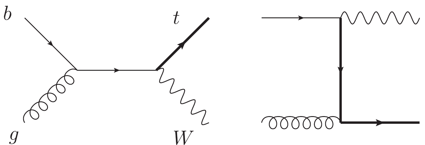Figure1. Leading order Feynman diagrams for $ gb\to tW $.

In comparison with experimental results, precision theoretical predictions are indispensable. The fixed-order corrections have been computed only up to the next-to-leading order in QCD for both the stable $ tW $ final state [8-11] or the process with their decays [12]. The parton shower and soft gluon resummation effects have been investigated in [13-15] and [16], respectively. Expanding the all-order formula of the threshold resummation to fixed orders, the approximate next-to-next-to-next-to-leading order total cross section has been obtained [17-20].
In the real corrections for $ tW^- $ production, there is a contribution from the $ gg(q\bar{q})\to tW^-{\bar b} $ channel, which can interfere with the top quark pair production $ gg(q\bar{q})\to t\bar{t} $, followed by the decay $ \bar{t}\to W^-{\bar b} $. These resonance effects make the higher-order correction excessively large, such that the perturbative expansion is no longer valid. Several methods have been proposed in the literature to address this problem. The Feynman diagrams containing two top quark resonances can be simply removed if the gauge dependence is negligible [13]. In a gauge invariant manner, the contribution of the $ t\bar{t} $ on-shell production and decay can be subtracted from the total $ tW(b) $ cross section either globally [9, 21] or locally [13, 14]. The interference can also be suppressed by simply choosing special cuts on the final-state particles [12, 22-24], such that there is a clear definition of the $ tW $ production channel. Refer to [25] for a review of these methods and implementation in MadGraph5_aMC@NLO.
To date, the exact next-to-next-to-leading order QCD corrections remain unavailable, although the next-to-next-to-leading order N-jettiness soft function of this process, one of the ingredients for a full next-to-next-to-leading order differential calculation using a slicing method, has been calculated in [26, 27]. The main bottleneck is the two-loop virtual correction, which involves multiple scales. The objective of this paper is to start the first step toward addressing this problem.
The last few decades have witnessed impressive progress in the understanding of the structure underlying the scattering amplitude, as well as the calculation of multi-loop Feynman integrals. For a specific process at a collider, the corresponding Feynman integrals can be categorized into different families according to their propagator configurations. Then, the integrals in each family can be reduced to a small set of basis integrals, which are called master integrals, by making use of the algebraic relationships among them, such as the identities generated via Integration by Parts (IBP) [28]. The number of master integrals has proven to be finite [29]. This IBP reduction procedure has been implemented in public computer programs, such as $ {\tt AIR}$ [30], $ {\tt Reduze}$ [31], $ {\tt LiteRed}$ [32], $ {\tt FIRE}$ [33], and $ {\tt Kira}$ [34], based on the Laporta algorithm [35]. Consequently, the main objective is to evaluate the master integrals either analytically or numerically; refer to recent reviews [36, 37]. For multi-loop integrals with multiple scales, it turns out that the differential equation is an efficient analytic method [38, 39], as it avoids the direct loop integration, which is rather complicated in some cases, by transforming the problem to determining a solution for a set of partial differential equations. This method has become widely adopted in many multi-loop calculations after the observation that the differential equations can be significantly simplified after selecting a canonical basis [40].
The remainder of this paper is organized as follows. In Sec. II, we present the canonical basis and corresponding differential equations. Subsequently, we discuss the determination of boundary conditions and present the analytical results in Sec. III. Finally, the conclusion is presented in Sec. IV.

The $ g(k_1)b(k_2)\to W(k_3)t(k_4) $ process contains two massive final states with different masses. For the external particles, there are on-shell conditions $ k_1^2 = 0, \; k_2^2 = 0, $$ k_3^2 = m_W^2 $ and $ k_4^2 = (k_1+k_2-k_3)^2 = m_t^2 $. The Mandelstam variables are defined as

$ s = (k_1+k_2)^2\,, \qquad t = (k_1-k_3)^2\,, \qquad u = (k_2-k_3)^2, \, $

(1)

with $ s+t+u = m_W^2+m_t^2 $. For later convenience, we define dimensionless variables y and z as

$ t = y\, m_t^2,\, \quad m_W = z\, m_t\,. $

(2)

It is usually believed that the more massive propagators a diagram involves, the more complicated the result is. The two-loop virtual corrections can have up to four massive propagators. Therefore, it is natural to divide the calculation to different parts according to the number of the massive propagators. In this study, we first focus on the diagrams with a single massive propagator. Figure 2 presents two of such diagrams with a double box topology, one being planar and the other non-planar. We solely discuss the planar diagram in the main text, leaving the non-planar diagram to the appendix. The amplitude of the planar diagram has been reduced to ten form factors in [41].
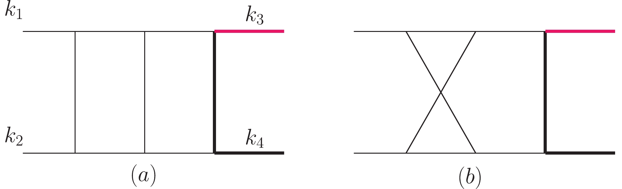Figure2. (color online) Planar (a) and non-planar (b) diagrams of the two-loop master integrals for $ gb\to Wt $ with one massive propagator. The massive external momenta are defined by $ k_3^2 = m_W^2,\; k_4^2 = m_t^2 $, and we consider that $ k_1,\;k_2 $ are ingoing while $ k_3,\;k_4 $ are outgoing.

We define the planar integral family, including the master integral presented in Fig. 2(a), in the form of

$\begin{aligned}[b] I_{n_1,n_2,\ldots,n_{9}} =& \int{\cal{D}}^D q_1\; {\cal{D}}^D q_2\\&\times\frac{1}{D_1^{n_1}\; D_2^{n_2}\; D_3^{n_3}\; D_4^{n_4}\; D_5^{n_5}\; D_6^{n_6}\; D_7^{n_7}D_8^{n_8}\; D_9^{n_9}}, \end{aligned}$

(3)

with

$ {\cal{D}}^D q_i = \frac{\left(m_t^2 \right)^\epsilon}{{\rm i} \pi^{D/2}{\rm e}^{-\epsilon\,\gamma_E}} d^D q_i \ ,\quad D = 4-2\epsilon \,. $

(4)

The nine denominators are given by

$ \begin{aligned}& D_1 = q_1^2,\quad\;\; D_2 = q_2^2,\quad\;\; D_3 = (q_1-k_1)^2, \\& D_4 = (q_1+k_2)^2,\quad\;\; D_5 = (q_1+q_2-k_1)^2,\\& D_6 = (q_2-k_1-k_2)^2,\\& D_7 = (q_2-k_3)^2-m_t^2,\\& D_8 = (q_1+k_1+k_2-k_3)^2-m_t^2,\\& D_9 = (q_2-k_1)^2. \end{aligned} $

Owing to momentum conservation, $ k_4 $ is not required in the denominators. The first seven denominators can be read directly from Fig. 2(a). The last two are added to form a complete basis for all Lorentz scalars that can be constructed from two loop momenta and three independent external momenta. The denominators $ D_8,D_9 $ solely appear with non-negative powers. They take a form that vanishes when the loop momentum, $ q_1 $ or $ q_2 $, becomes soft, and therefore they are less divergent. In addition, the choice of $ D_9 $ can be justified following the method in [42]. If we put the four massless propagators containing $ q_1 $ on-shell, then we obtain a Jacobian

$ J = \frac{1}{(k_1+k_2)^2 (q_2-k_1)^2}. $

(5)

From the one-loop calculation, we know that the remaining three uncut propagators containing $ q_2 $ already form an MI in the ?-form (up to a factor depending on the external momenta). Therefore, a $ D_9 $ in the numerator would just cancel the hidden $ q_2 $ propagator in the Jacobian.
Making use of the $ {\tt FIRE}$ package, we determine that the integrals in the planar family can be reduced to a basis of 31 MIs after considering the symmetries between integrals. We first select the MIs in such a form that the differential equations have coefficients linear in ?. These MIs are given by

$\begin{aligned}[b]{{{M}}_1} =&\; {\epsilon ^2}{\mkern 1mu} {I_{0,0,0,1,2,0,2,0,0}}{\mkern 1mu} ,\quad{{{M}}_2} = {\epsilon ^2}{\mkern 1mu} {I_{0,0,1,0,2,0,2,0,0}}{\mkern 1mu} ,\\{{{M}}_3} = &\;{\epsilon ^2}{\mkern 1mu} {I_{0,0,2,0,2,0,1,0,0}}{\mkern 1mu} ,\quad{{{M}}_4} = {\epsilon ^2}{\mkern 1mu} {I_{0,0,1,0,2,2,0,0,0}}{\mkern 1mu} ,\\{{{M}}_5} =&\; {\epsilon ^3}{\mkern 1mu} {I_{0,0,1,0,2,1,1,0,0}}{\mkern 1mu} ,\quad{{{M}}_6} = {\epsilon ^2}{\mkern 1mu} {I_{0,0,1,2,0,0,2,0,0}}{\mkern 1mu} ,\\{{{M}}_7} =&\;{\epsilon ^3}{\mkern 1mu} {I_{0,0,1,1,1,0,2,0,0}}{\mkern 1mu} ,\quad{{{M}}_8} = {\epsilon ^2}{\mkern 1mu} {I_{0,0,1,1,1,0,3,0,0}}{\mkern 1mu} ,\\{{{M}}_9} =&\; {\epsilon ^2}{\mkern 1mu} {I_{0,0,2,1,1,0,2,0,0}}{\mkern 1mu} ,\quad{{{M}}_{10}} = {\epsilon ^3}{\mkern 1mu} {I_{0,1,0,1,2,0,1,0,0}}{\mkern 1mu} ,\\{{{M}}_{11}} =&\; {\epsilon ^2}{\mkern 1mu} {I_{0,1,0,1,2,0,2,0,0}}{\mkern 1mu} ,\quad{{{M}}_{12}} = {\epsilon ^2}{\mkern 1mu} {I_{0,1,1,2,0,0,2,0,0}}{\mkern 1mu} ,\\{{{M}}_{13}} =&\; {\epsilon ^2}{\mkern 1mu} {I_{0,1,1,2,0,2,0,0,0}}{\mkern 1mu} ,\quad{{{M}}_{14}} = {\epsilon ^3}{\mkern 1mu} {I_{0,1,1,2,0,1,1,0,0}}{\mkern 1mu} ,\\{{{M}}_{15}} =&\; {\epsilon ^4}{\mkern 1mu} {I_{0,1,1,1,1,0,1,0,0}}{\mkern 1mu} ,\quad{{{M}}_{16}} = {\epsilon ^2}{\mkern 1mu} {I_{1,0,0,0,2,0,2,0,0}}{\mkern 1mu} ,\\{{{M}}_{17}} =&\; {\epsilon ^2}{\mkern 1mu} {I_{2,0,0,0,2,0,1,0,0}}{\mkern 1mu} ,\quad{{{M}}_{18}} = {\epsilon ^4}{\mkern 1mu} {I_{1,0,1,0,1,1,1,0,0}}{\mkern 1mu} ,\\{{{M}}_{19}} = &\;{\epsilon ^3}{\mkern 1mu} {I_{1,0,1,0,1,1,2,0,0}}{\mkern 1mu} ,\quad{{{M}}_{20}} = {\epsilon ^3}{\mkern 1mu} {I_{1,0,1,1,1,0,2,0,0}}{\mkern 1mu} ,\\{{{M}}_{21}} =&\; {\epsilon ^2}{\mkern 1mu} {I_{1,0,1,1,1,0,3,0,0}}{\mkern 1mu} ,\quad{{{M}}_{22}} = {\epsilon ^3}{\mkern 1mu} {I_{1,1,0,0,2,0,1,0,0}}{\mkern 1mu} ,\\{{{M}}_{23}} =&\; {\epsilon ^3}{\mkern 1mu} {I_{1,1,0,0,2,1,0,0,0}}{\mkern 1mu} ,\quad{{{M}}_{24}} = {\epsilon ^3}(1 - 2\epsilon ){\mkern 1mu} {I_{1,1,0,0,1,1,1,0,0}}{\mkern 1mu} ,\\{{{M}}_{25}} =&\; {\epsilon ^3}{\mkern 1mu} {I_{1,1,0,0,2,1,1,0,0}}{\mkern 1mu} ,\quad{{{M}}_{26}} = {\epsilon ^4}{\mkern 1mu} {I_{1,1,0,1,1,0,1,0,0}}{\mkern 1mu} ,\\{{{M}}_{27}} =&\; {\epsilon ^3}{\mkern 1mu} {I_{1,1,0,1,1,0,2,0,0}}{\mkern 1mu} ,\quad{{{M}}_{28}} = {\epsilon ^4}{\mkern 1mu} {I_{1,1,1,1,1,0,1,0,0}}{\mkern 1mu} ,\\{{{M}}_{29}} =&\; {\epsilon ^4}{\mkern 1mu} {I_{1,1,1,1,1,1,1,0,0}}{\mkern 1mu} ,\quad{{{M}}_{30}} = {\epsilon ^4}{\mkern 1mu} {I_{1,1,1,1,1,1,1,0, - 1}}{\mkern 1mu} ,\\{{{M}}_{31}} =&\; {\epsilon ^4}{\mkern 1mu} {I_{1,1,1,1,1,1,1, - 1,0}}{\mkern 1mu} .\end{aligned}$

(6)

The corresponding topology diagrams are displayed in Fig. 3.
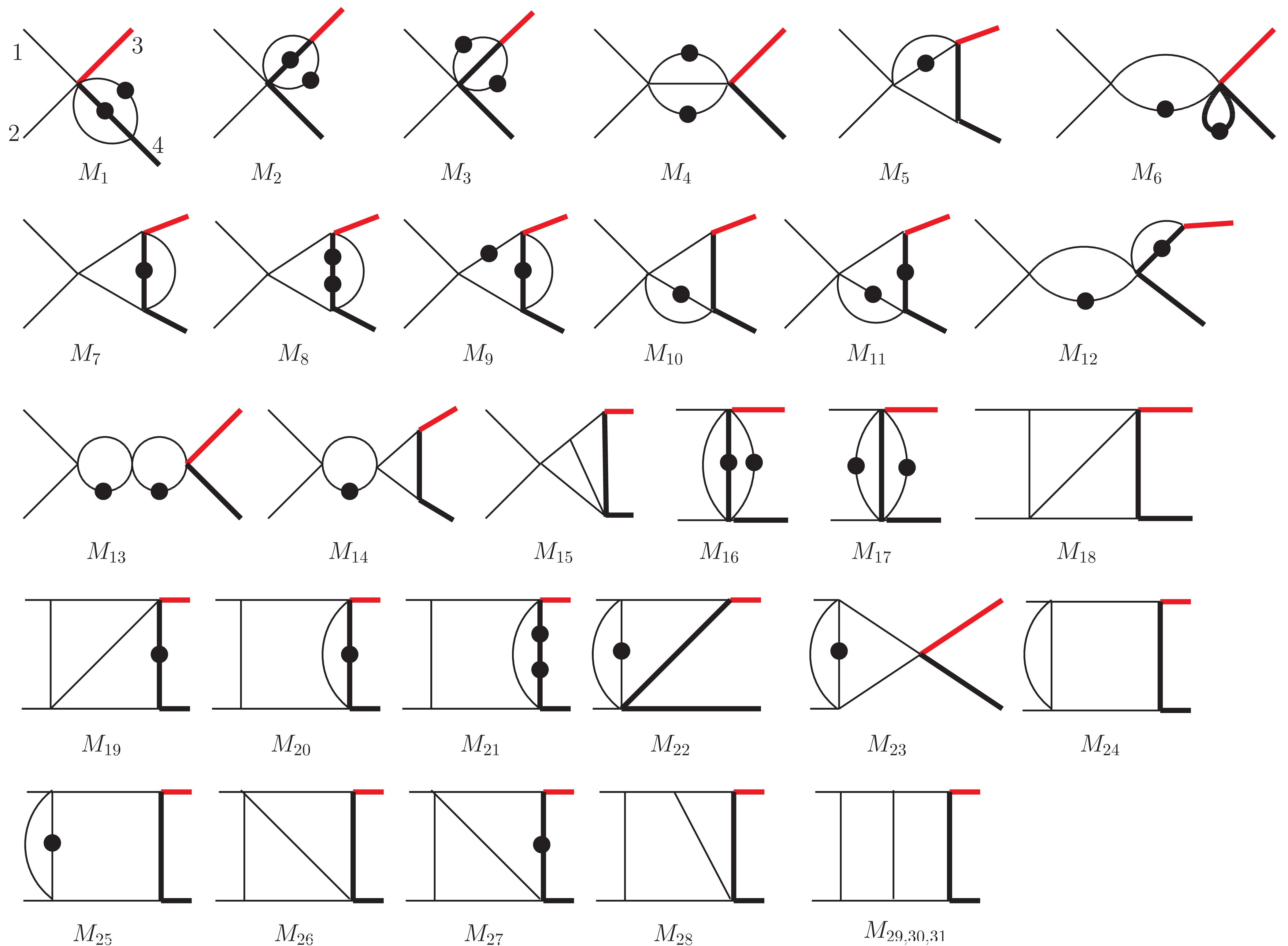Figure3. (color online) Master integrals in the planar family. The thin and thick lines represent massless and massive particles, respectively. The red line in the final state denotes W. Each block dot indicates one additional power of the corresponding propagator. Numerators are not shown explicitly in the diagram and could be found in the text.

Subsequently, we transform the MIs to a canonical basis using a method similar to that described in [43], starting from the lower sectors (with fewer propagators) to higher sectors (with more propagators). The main logic is to consider the ? parts in the differential equations as perturbations. After solving the differential equation in four dimensions, i.e., omitting the perturbations, we obtain the dominant part of the MIs. Then the full solution can be obtained by using the variation of constants method. The coefficient functions varied from the constants satisfy the canonical form of differential equations. For the integrals in the same sector, we have selected a basis, such that the differential equations vanish in four dimensional spacetime. For example, $ F_2 $ and $ F_3 $ belong to the same sector. They satisfy differential equations

$ \begin{aligned}[b] \frac{\text{d} {M}_{2} }{\text{d} z} =& -\frac{2(1+\epsilon)}{z} {M}_2-\frac{2\epsilon}{z} {M}_3,\\ \frac{\text{d} {M}_{3} }{\text{d} z} =& \left(\frac{4(1+\epsilon)}{z}-\frac{2(1+\epsilon)}{z-1}-\frac{2(1+\epsilon)}{z+1}\right) {M}_2\\&+ \left(\frac{4\epsilon}{z}-\frac{1+4\epsilon}{z-1}-\frac{1+4\epsilon}{z+1}\right) {M}_3 . \end{aligned} $

(7)

Solving the above equations at $ \epsilon = 0 $, we deduce that the differential equations for the new basis

$ \begin{aligned}[b]{F}_{2} =&\; m_W^2 \, {M}_2\,, \\ {F}_{3} =&\; (m_W^2-m_t^2) \, {M}_3-2m_t^2\, {M}_2,\,\end{aligned} $

(8)

are vanishing at $ \epsilon = 0 $. Going back to the $ 4-2\epsilon $ dimension, we have

$ \begin{aligned}[b] \frac{\text{d} {F}_{2} }{\text{d} z} =&\; \epsilon\left(\frac{2 {F}_{2}}{z}-\frac{2 {F}_{2}+ {F}_{3}}{z-1}-\frac{2 {F}_{2}+ {F}_{3}}{z+1}\right),\\ \frac{\text{d} {F}_{3} }{\text{d} z} =&\; \epsilon\left(\frac{8 {F}_{2}}{z}-2\frac{2 {F}_{2}+ {F}_{3}}{z-1}-2\frac{2 {F}_{2}+ {F}_{3}}{z+1}\right), \end{aligned} $

(9)

where the parameter ? of the spacetime dimension appears only as a multiplicative factor on the right hand side of the differential equations, which is called the canonical or $ d\ln $ form [40].
Accordingly, we obtain the following MIs that satisfy canonical differential equations.

$ \begin{aligned}[b] {F}_{1} =&\; m_t^2 {M}_1\,, \qquad {F}_{2} = m_W^2 \, {M}_2\,, \qquad {F}_{3} = (m_W^2-m_t^2) \, {M}_3-2m_t^2\, {M}_2\,, \qquad {F}_{4} = (-s)\, {M}_4\,, \qquad {F}_{5} = r_1 \, {M}_5 \,, \qquad {F}_{6} = (-s)\, {M}_6\,,\\ {F}_{7} =&\; r_1 \, {M}_7\,, \qquad {F}_{8} = m_t^2 r_1 \, {M}_8\,, \qquad {F}_{9} = m_W^2 s\, {M}_9+m_t^2(m_t^2-m_W^2-s)\, {M}_8+\frac{3}{2}(m_t^2-m_W^2-s)\, {M}_7\,, \\ {F}_{10} =&\; r_1 \, {M}_{10}\,, \qquad {F}_{11} = m_t^2(-s)\, {M}_{11}-\frac{3}{2}(m_t^2-m_W^2+s)\, {M}_{10}\,, \qquad {F}_{12} = m_W^2\,s\, {M}_{12}\,, \qquad {F}_{13} = s^2\, {M}_{13}\,, \\ {F}_{14} =&\; (- s)\,r_1 \, {M}_{14}\,, \qquad {F}_{15} = r_1 \, {M}_{15}\,, \qquad {F}_{16} = t \, \text{M}_{16}\,, \qquad {F}_{17} = (t-m_t^2)\, {M}_{17}-2m_t^2\, {M}_{16}\,, \qquad {F}_{18} = (m_W^2-s-t) \, {M}_{18}\,, \\ {F}_{19} =&\; m_t^2(-s) \, {M}_{19}\,,\qquad {F}_{20} = t\,(-s) {M}_{20}\,, \qquad {F}_{21} = m_t^2(-s)\left((t-m_t^2) {M}_{21}- {M}_{20}\right)\,, \qquad {F}_{22} = (t-m_W^2) \, {M}_{22}\,, \\ {F}_{23} = &\;(-s) \, {M}_{23}\,, \qquad {F}_{24} = r_1 \, {M}_{24}\,, \qquad {F}_{25} = (t-m_t^2)(-s)\, {M}_{25}\,, \qquad {F}_{26} = (m_t^2-s-t) \, {M}_{26}\,, \\ {F}_{27} =&\; -(m_W^2\,t-m_t^2(s+t+m_W^2)+m_t^4)\, {M}_{27}\,, \qquad {F}_{28} = (t-m_W^2)(-s) \, {M}_{28}\,, \qquad {F}_{29} = -(t-m_t^2)s^2\, {M}_{29}\,, \qquad {F}_{30} = (-s)r_1 \, {M}_{30}\,, \\ {F}_{31} =&\; s^2 \,( {M}_{31}+ {M}_{14})+s\,\left(- {M}_{15}- {M}_{10}+2 {M}_{7}-\frac{3}{2} {M}_{5}+3m_t^2\, {M}_{8}\right) +(s+t-m_W^2)\left(s\, {M}_{25}-\frac{1}{4} {M}_{17}\right)-\frac{s+t-m_W^2}{4(t-m_t^2)}[2(m_t^2+2m_W^2)\, {M}_{2}\\&\;-3s\, {M}_{4}+(m_t^2-m_W^2) {M}_{3}-2(2t+m_t^2) {M}_{16}+12(s+t-m_W^2) {M}_{18}+8m_t^2\,s\, {M}_{19}]. \end{aligned}$

(10)

The combination coefficients are generally just rational functions in $ s,t,m_W^2,m_t^2 $, except the square root product $ r_1\equiv \sqrt{s-(m_t-m_W)^2}\sqrt{s-(m_t+m_W)^2} $ in the basis integrals such as $ F_5,\;F_7 $. This square root also appears in the differential equations. It is necessary to first rationalize the square root before solving the differential equations in terms of multiple polylogarithms. To achieve this objective, we perform the following change of integration variable,

$ s = m_t^2\frac{(x+z)(1+x z)}{x} $

(11)

with $ -1<x<1 $ so that $ r_1 = (1-x)(1+x)z/x $. Note that $ r_1 $ is negative (positive) when s is negative (positive). Here, we also select $ m_W $ or z as a variable because it is easy to determine the boundary conditions for some integrals at $ z = 0 $. Hence, the differential equations for $ {\boldsymbol{F}} = ( {F}_1,\ldots , {F}_{31}) $ can be written as

$ { d}\, {\boldsymbol{F}}(x,y,z;\epsilon) = \epsilon\, ({ d} \, \tilde{A})\, {\boldsymbol{F}}(x,y,z;\epsilon), $

(12)

with

$ {d}{\mkern 1mu} \tilde A = \sum\limits_{i = 1}^{15} {{R_i}} {\mkern 1mu} { d}\ln ({l_i}), $

(13)

where $ R_i $ are rational matrices. Their explicit forms are provided in an auxiliary file. The arguments $ l_i $ of this d ln form, which contain the entire dependence of the differential equations on the kinematics, are referred to as the alphabet, and they consist of the following letters:

$ \begin{aligned}[b] l_1 =&\; x\,,\qquad l_2 = x+1\,, \qquad l_3 = x-1\,, \qquad l_4 = x+z\,, \\ l_5 = &\;x\,z+1\,,\quad l_6 = x\; y+z\,, \quad l_7 = x\,z+y \,,\quad l_8 = y \, , \\ l_9 =&\; y-1\,,\qquad l_{10} = y-z^2\, , \qquad l_{11} = z\,,\qquad l_{12} = z^2-1\, , \\ l_{13} =&\; x^2 z+x y+x+z \,,\qquad l_{14} = x^2 z+x \left(y+z^2\right)+z \, , \\ l_{15} =&\; x^2 z+x \left(-y z^2+y+2 z^2\right)+z \,, \qquad l_{16} = x^2 z+x y+z\,, \\l_{17} =&\; x^2 z^3+x y \left(z^2-1\right)+2 x z^2+z^3 . \end{aligned} $

(14)

Notice that the last two letters, $ l_{16} $ and $ l_{17} $, only appear for the non-planar integral family discussed in the appendix.
Because the roots of the letters above are purely algebraic, the solutions of the differential equations can be directly expressed in terms of multiple polylogarithms [44], which are defined as $ G(x)\equiv 1 $ and

$ G_{a_1,a_2,\ldots,a_n}(x) \equiv \int_0^x \frac{\text{d} t}{t - a_1} G_{a_2,\ldots,a_n}(t)\, , $

(15)

$ G_{\overrightarrow{0}_n}(x) \equiv \frac{1}{n!}\ln^n x\, . $

(16)

The length n of the vector $ (a_1,a_2,\ldots,a_n) $ is regarded as the transcendental $ weight $ of multiple polylogarithms.

To obtain the analytical solutions of the differential equations for the canonical basis presented above, we need to fix the boundary conditions first.
The base $ {F}_1 $ is directly obtained by integration, which can also be found in [45].

$ {F}_1 = -\frac{1}{4}-\epsilon^2\frac{5\pi^2}{24}-\epsilon^3\frac{11\zeta(3)}{6}-\epsilon^4\frac{101\pi^4}{480}+{\cal{O}}(\epsilon^{5}). $

(17)

The loop integrals in the planar family do not have a branch cut at $ m_W = 0\; (z = 0) $. Therefore, the corresponding canonical differential equations should not have a pole at $ z = 0 $. This regularity condition provides useful information about the boundaries. As can be observed from Eq. (9), the coefficient of $ 1/z $ should vanish at $ z = 0 $, which means $ F_2|_{z = 0} = 0 $. Owing to the same reason, the bases $ {F}_9 $ and $ {F}_{12} $, also vanish at $ z = 0 $, and

$ {F}_{11}\Big|_{z = 0} = \left( {F}_{1}-\frac{ {F}_{4}}{2}\right)\bigg|_{z = 0} \,. $

(18)

The boundary condition for $ {F}_3 $ at $ z = 0 $ is calculated directly,

$ {F}_{3}\Big|_{z = 0} = 1+\epsilon^2\frac{\pi^2}{2}-\epsilon^3\frac{8\zeta(3)}{3}+\epsilon^4\frac{7\pi^4}{40}+{\cal{O}}(\epsilon^{5}). $

(19)

In the bases $ \{ {F}_4, {F}_{23}\} $, the final-state W boson and top quark can be considered a single particle. All the propagators are massless, and they appear in the massless double box diagrams. Here we independently derive their values at $ s = m_t^2 $, which can be used as the boundary at $ z = 0,\;x = 1 $.

$ \begin{aligned}[b] {F}_{4}\Big|_{s = {m_t^2}} =&\; -1-2\epsilon\, {\rm i}\, \pi+\epsilon^2\frac{13\pi^2}{6}+\epsilon^3\frac{32\zeta(3)+5 {\rm i} \pi^3}{3}\\&\;+\epsilon^4\left(-\frac{101\pi^4}{120}+\frac{64 {\rm i}\, \pi\, \zeta(3)}{3}\right)+{\cal{O}}(\epsilon^{5}), \\ {F}_{23}\Big|_{s = m_t^2} =&\; \frac{1}{4}+\epsilon\, \frac{{\rm i}\, \pi}{2}-\epsilon^2\frac{11\pi^2}{24}-\epsilon^3\left(\frac{13\zeta(3)}{6}+\frac{ {\rm i} \pi^3}{4}\right) \\&\;+\epsilon^4\left(\frac{79\pi^4}{1440}-\frac{13 {\rm i}\, \pi\, \zeta(3)}{3}\right)+{\cal{O}}(\epsilon^{5}) . \end{aligned} $

The bases $ \{ {F}_6, {F}_{13}\} $ factorize to a product of two one-loop integrals, and can be computed easily,

$ \begin{aligned}[b] {F}_{6}\Big|_{s = m_t^2} =&\; 1+\epsilon\, {\rm i}\, \pi-\epsilon^2\frac{\pi^2}{2}-\epsilon^3\frac{16\zeta(3)+{\rm i} \pi^3}{3}\\&\;+\epsilon^4\left(\frac{\pi^4}{120}-\frac{8 {\rm i}\, \pi\, \zeta(3)}{3}\right)+{\cal{O}}(\epsilon^{5}), \\ {F}_{13}\Big|_{s = m_t^2} =&\; 1+ 2\epsilon\, {\rm i}\, \pi-\epsilon^2\frac{13\pi^2}{6}-\epsilon^3\frac{14\zeta(3)+5 {\rm i} \pi^3}{3}\\&\;+\epsilon^4\left(\frac{113\pi^4}{120}-\frac{28 {\rm i}\, \pi\, \zeta(3)}{3}\right)+{\cal{O}}(\epsilon^{5})\,. \end{aligned} $

The integrals of $\{ {F}_{5}, {F}_{7}, {F}_{8}, {F}_{10}, {F}_{14}, F}_{15}, {F}_{24}, {F}_{30}\}$ are multiplied by $ r_1 $ in the basis, and thus they vanish at $ x = 1 $.
The bases $ \{ {F}_{16}, {F}_{17}\} $ are the same as $ \{ {F}_{2}, {F}_{3}\} $ after replacing t by $ m_W^2 $. Hence, their boundaries at $ y = 0 $ are known from $ \{ {F}_{2}, {F}_{3}\} $ at $ z = 0 $.
From the definitions of the bases, we know that $ {F}_{18}, $$ {F}_{22},\;{F}_{26},\; {F}_{27} $ vanish at $ u = m_t^2\; (l_{13} = 0),\;t = m_W^2\; (y = z^2), $$ u = m_W^2\, (l_{14} = 0),\;m_W^2\,t-m_t^2(s+t+m_W^2)+m_t^4 = 0\; (l_{15} = 0) $, respectively.
The boundary conditions of $ \{ {F}_{19}, {F}_{20}, {F}_{21}, {F}_{25}, {F}_{28}, $$ {F}_{29}, {F}_{31}\} $ are determined from the regularity conditions at $ u\, t = m_t^2\,m_W^2 \; (x = -\dfrac{y}{z}) $.
With the discussion above, we determine all the boundary conditions for the planar family. Accordingly, the analytic results of the basis from the canonical differential equations can be obtained directly. We provide the results of the MIs in electronic form in the ancillary files attached to the arXiv submission of the paper. Below we express the first two terms in the expansion of ?.

$ \begin{aligned}[b] {F}_1 =&\; -\frac{1}{4} + \epsilon \cdot 0 +{\cal{O}}(\epsilon^2)\,, \qquad {F}_2 = 0 - \epsilon \cdot \ln \left(1-z^2\right)+{\cal{O}}(\epsilon^2)\,, \\ {F}_3 =&\; 1 - \epsilon \cdot 2 \ln \left(1-z^2\right)+{\cal{O}}(\epsilon^2)\,, \\ {F}_4 =&\; -1 + \epsilon \cdot 2 \ln \left(\frac{(x+z) (x z+1)}{x}\right)-2 {\rm i} \pi +{\cal{O}}(\epsilon^2)\,, \\ {F}_5 = &\;0 - \epsilon \cdot 0+{\cal{O}}(\epsilon^2) \,, \\ {F}_6 =&\; 1 - \epsilon \cdot \ln \left(\frac{(x+z) (x z+1)}{x}\right)+{\rm i} \pi +{\cal{O}}(\epsilon^2)\,, \\ {F}_7 =&\; 0 + \epsilon \cdot 0 +{\cal{O}}(\epsilon^2)\,, \qquad {F}_8 = 0 + \epsilon \cdot 0 +{\cal{O}}(\epsilon^2)\,, \\ {F}_9 =&\; 0 - \epsilon \cdot \ln \left(1-z^2\right)+{\cal{O}}(\epsilon^2)\,, \qquad \text{F}_{10} = 0 + \epsilon \cdot 0 +{\cal{O}}(\epsilon^2)\,, \\ {F}_{11} = &\;\frac{1}{4} + \epsilon \cdot \left[ -\ln \left(\frac{(x+z) (x z+1)}{x}\right)+\ln\left(1-z^2\right)+{\rm i} \pi \right]+{\cal{O}}(\epsilon^2)\,, \\ {F}_{12} =&\; 0 - \epsilon \cdot \ln \left(1-z^2\right)+{\cal{O}}(\epsilon^2)\,, \\ {F}_{13} =&\; 1 + \epsilon \cdot \left[ -2 \ln \left(\frac{(x+z) (x z+1)}{x}\right)+2 {\rm i} \pi \right]+{\cal{O}}(\epsilon^2)\,, \\{F}_{14} =&\; 0 + \epsilon \cdot 0+{\cal{O}}(\epsilon^2)\,, \\ {F}_{15} =&\; 0 + \epsilon \cdot 0 +{\cal{O}}(\epsilon^2)\,, \qquad {F}_{16} = 0 - \epsilon \cdot \ln (1-y)+{\cal{O}}(\epsilon^2)\,, \\ {F}_{17} =&\; 1 - \epsilon \cdot 2 \ln(1-y)+{\cal{O}}(\epsilon^2)\,, \qquad {F}_{18} = 0 + \epsilon \cdot 0+{\cal{O}}(\epsilon^2)\,, \\ {F}_{19} =&\; -\frac{1}{6} + \epsilon \cdot \left[ \frac{1}{2} \ln \left(\frac{(x+z) (x z+1)}{x}\right)-\frac{1}{3} \ln (1-y)-\frac{{\rm i} \pi }{2}\right]\\&+{\cal{O}}(\epsilon^2)\,, \\ {F}_{20} =&\; 0 - \epsilon \cdot \ln (1-y)+{\cal{O}}(\epsilon^2)\,, \\ {F}_{21} =&\; \frac{5}{8} + \epsilon \cdot \left[ -\frac{1}{2} \ln \left(\frac{(x+z) (x z+1)}{x}\right)-\ln (1-y)\right.\\&+\left.\frac{1}{2} \ln \left(1-z^2\right)+\frac{{\rm i} \pi }{2} \right]+{\cal{O}}(\epsilon^2)\,, \end{aligned}$

$ \begin{aligned}[b] {F}_{22} =&\; 0 + \epsilon \cdot \left[ \frac{1}{2} \ln (1-y)-\frac{1}{2} \ln \left(1-z^2\right) \right]+{\cal{O}}(\epsilon^2)\,, \\ {F}_{23} = &\;\frac{1}{4} + \epsilon \cdot \left[ -\frac{1}{2} \ln \left(\frac{(x+z) (x z+1)}{x}\right)+\frac{{\rm i} \pi }{2}\right]+{\cal{O}}(\epsilon^2)\,, \\ {F}_{24} =&\; 0 + \epsilon \cdot 0+{\cal{O}}(\epsilon^2)\,, \\ {F}_{25} = &\;\frac{5}{12} + \epsilon \cdot \left[ -\frac{1}{2} \ln \left(\frac{(x+z) (x z+1)}{x}\right)-\frac{7}{6} \ln (1-y)\right.\\&\;\left.+\frac{1}{2} \ln \left(1-z^2\right)+\frac{{\rm i} \pi }{2} \right]+{\cal{O}}(\epsilon^2)\,, \\ {F}_{26} = &\;0 + \epsilon \cdot 0 +{\cal{O}}(\epsilon^2)\,, \qquad {F}_{27} = 0 + \epsilon \cdot 0 +{\cal{O}}(\epsilon^2)\,, \\ {F}_{28} =&\; 0 + \epsilon \cdot \left[ \frac{1}{2} \ln(1-y)-\frac{1}{2} \ln \left(1-z^2\right) \right]+{\cal{O}}(\epsilon^2)\,, \\ {F}_{29} =&\; -\frac{11}{24} + \epsilon \cdot \left[ \frac{1}{2} \ln \left(\frac{(x+z) (x z+1)}{x}\right)+\frac{4}{3} \ln (1-y)\right.\\&\;\left.-\frac{1}{2} \ln \left(1-z^2\right)-\frac{{\rm i} \pi }{2} \right]+{\cal{O}}(\epsilon^2)\,, \\ {F}_{30} =&\; 0 + \epsilon \cdot 0 +{\cal{O}}(\epsilon^2)\,, \qquad {F}_{31} = \frac{1}{24} - \epsilon \cdot \frac{1}{6} \ln (1-y)+{\cal{O}}(\epsilon^2)\,. \end{aligned}$

(20)

In our calculation, we have varied $ m_W $ to select a proper boundary condition. A question on the possibility of taking the boundary $ m_W = m_t $, equivalently $ z = 1 $, can be asked. If the answer is yes, then all the results of the two-loop integrals can be adopted for $ gg\to t\bar{t} $. However, this is non-trivial because $ z = 1 $ is the point where a branch cut starts. For example, we can take $ F_1 $ as a boundary for $ F_2 $ at $ z = 1 $ because they are the same if setting $ m_W^2 = m_t^2 $ in the integrands. However, we see from the above analytic results expanded in ? that $ {F_2}|_{z = 1}\neq F_1 $. The reason is that the analytic results are valid only for $ z^2<1 $. In the $ z\to1 $ limit, the $ (1-z)^{n\epsilon} $ terms cannot be expanded in a series of ? for the master integrals. Instead, the differential equation in Eq. (9) should be solved with full ? dependence,

$ \begin{aligned}[b]{F}_{2} =\; c_1 (1-z)^{-4\epsilon} -c_2 , \quad {F}_{3} = \;2c_1 (1-z)^{-4\epsilon} +2c_2 . \end{aligned} $

(21)

Comparing these with the analytic results in Eq. (20), we deduce that

$ c_1 = \frac{1}{4}-\epsilon \ln 2+{\cal{O}}(\epsilon^2) ,\quad c_2 = \frac{1}{4}+{\cal{O}}(\epsilon^2) . $

(22)

Subsequently, taking $ (1-z)^{-4\epsilon}\to 0 $ at $ z = 1 $, we infer that $ { {F}_2}|_{z = 1} ={F}_1 $. If the boundary values at $ z = 1 $ are adopted for $ {F}_2 $ and $ {F}_3 $, which are $ -c_2 $ and $ 2c_2 $, respectively, the $ c_1 $ information is still required to obtain the results at general z. However, this information can only be obtained at a point other than $ z = 1 $.
All the analytic results are real in the Euclidean regions $ (s<0,\;t<0,\;u<0) $. In this work we are interested in the physical region with $ s>(m_t+m_W)^2,\;t_0<t<t_1, $$ 0<m_W^2<m_t^2 $,^① where

$ t_0\equiv \frac{m_t^2+m_W^2-s-r_1}{2}, \qquad t_1\equiv \frac{m_t^2+m_W^2-s+r_1}{2}. $

(23)

This region corresponds to $ 0<x<1,\; -2z/x<y<-2zx, $$ 0<z<1 $. The analytic continuation to this region can be performed by assigning s a numerically small imaginary part $ i\varepsilon\,(\varepsilon>0) $, i.e., $ s\rightarrow s+i\varepsilon $. This prescription provides correct numerical results in both the Euclidean and physical regions, when the multiple polylogarithms are evaluated using ${\tt GiNaC}$ [46, 47].
All the analytical results have been checked with the numerical package ${\tt FIESTA}$ [48], and they agree within the computation errors in both Euclidean and physical regions. For example, we present the results of two integrals at a physical kinematic point $ (s = 10,\;t = -2, \; m_W^2 = \dfrac{1}{4}, $$ m_t = 1) $,

$ I_{1, 0, 1, 0, 1, 1, 1, 0, 0}^{\rm analytic} = \frac{0.00475421+ 1.48022009\,{\rm i}}{\epsilon} +(-5.24410651+1.22399295\,{\rm i}), $

(24)

$ \begin{aligned}[b] I_{1, 0, 1, 0, 1, 1, 1, 0, 0}^{\rm FIESTA} = \frac{0.004754+1.48022\, {\rm i}\pm0.000056(1+i) }{\epsilon}+(-5.24410 + 1.22399 \,{\rm i}) \, \pm (0.000416+0.000415\,{\rm i})\,,\end{aligned} $

(25)

and

$ \begin{aligned}[b] I_{1, 1, 1, 1, 1, 0, 1, 0, 0}^{\rm analytic} = \frac{0.0308065}{\epsilon^3}+\frac{-0.06040731}{\epsilon^2}+\frac{0.22341495-0.06475586\,{\rm i}}{\epsilon}+(-0.26302494 +0.62749975\,{\rm i}), \end{aligned}$

(26)

$ \begin{aligned}[b] I_{1, 1, 1, 1, 1, 0, 1, 0, 0}^{\rm FIESTA} =&\; \frac{0.030807 \pm0.000005 }{\epsilon^3}+\frac{-0.060407 \pm0.000027 }{\epsilon^2}+\frac{0.223415 -0.064756\, {\rm i} \pm(0.000116+0.000124 \,{\rm i}) }{\epsilon}\\&+(-0.263019 + 0.627484 \,{\rm i}) \, \pm (0.000392 + 0.000395 \,{\rm i}). \end{aligned} $

(27)

We analytically calculate two-loop master integrals for hadronic $ tW $ productions that solely contain one massive propagator. After choosing a canonical basis, the differential equations for the master integrals can be transformed into the dln form. The boundaries are determined by simple direct integrations or regularity conditions at kinematic points without physical singularities. The analytical results in this study are expressed in terms of multiple polylogarithms, and have been checked via numerical computations. A significant amount of work is still required in the future to obtain the complete two-loop virtual corrections in this channel.

For the master integral presented in Fig. 2(b), we define the non-planar integral family as

$\tag{A1}\begin{aligned}[b] J_{n_1,n_2,\ldots,n_{9}} =&\; \int{\cal{D}}^D q_1\; {\cal{D}}^D q_2\\&\times\frac{1}{P_1^{n_1}\; P_2^{n_2}\; P_3^{n_3}\; P_4^{n_4}\; P_5^{n_5}\; P_6^{n_6}\; P_7^{n_7}P_8^{n_8}\; P_9^{n_9}} \end{aligned} $

with the denominators

$ \begin{aligned}\\ P_1 =&\; q_1^2,\qquad P_2 = (q_1-q_2)^2,\qquad P_3 = q_2^2,\qquad P_4 = (q_1+k_1)^2,\qquad P_5 = (q_1-q_2-k_2)^2,\qquad P_6 = (q_2+k_1+k_2)^2,\\ P_7 =&\; (q_2+k_1+k_2-k_3)^2-m_t^2,\qquad P_8 = (q_1-k_3)^2,\qquad P_9 = (q_2+k_1)^2. \end{aligned}$

The canonical bases are selected to be

$\tag{A2} \begin{aligned}[b]{B}_{1} = &\; m_t^2 {N}_1\,,\quad {B}_{2} = m_W^2 \, {N}_2\,,\quad {B}_{3} = (m_W^2-m_t^2) \, {N}_3-2m_t^2\, {N}_2\,, \quad{B}_{4} = (-s)\, {N}_4\,, \quad {B}_{5} = r_1 \, {N}_5 \,, \quad {B}_{6} = (m_W^2+m_t^2-s-t)\, {N}_6\,, \\ {B}_{7} =&\; (m_W^2-s-t)\, {N}_7-2m_t^2\, {N}_6\,, \quad {B}_{8} = (m_W^2-s-t)\, {N}_8\,, \quad {B}_{9} = s\, {N}_9\,,\quad {B}_{10} = t\, {N}_{10}\,, \quad {B}_{11} = (t-m_t^2)\, {N}_{11}-2m_t^2\, {N}_{10}\,, \\ {B}_{12} =&\; (t-m_W^2)\, {N}_{12}\,, \quad {B}_{13} = r_1 \, {N}_{13}\,, \quad {B}_{14} = m_t^2(-s)\, {N}_{14}-\frac{3}{2}(m_t^2-m_W^2+s)\, {N}_{13}\,, \quad {B}_{15} = r_1 \, {N}_{15}\,, \quad {B}_{16} = s(s+t-m_W^2) \, {N}_{16}\,, \\ {B}_{17} =&\; (t-m_t^2)\, {N}_{17}\,, \quad {B}_{18} = m_t^2(-s) \, {N}_{18}\,, \quad{B}_{19} = r_1 \, {N}_{19}\,, \quad {B}_{20} = (t-m_t^2)(-s) \, {N}_{20}\,, \quad {B}_{21} = (m_W^2-s-t)\, {N}_{21}\,, \\ {B}_{22} = &\;m_t^2(-s)\, {N}_{22}\,, \quad {B}_{23} = (m_t^2-s-t)\, {N}_{23}\,, \quad{B}_{24} = -(t\, m_W^2-(m_W^2+s+t)m_t^2+m_t^4)\, {N}_{24}\,, \quad{B}_{25} = (t-m_W^2)\, {N}_{25}\,, \\ {B}_{26} =&\; (m_W^2(s+t-m_W^2)-m_t^2(t-m_W^2))\, {N}_{26}\,, \quad {B}_{27} = (-s)\, {N}_{27}\,, \quad {B}_{28} = (t-m_t^2)(m_W^2-s-t)\, {N}_{28}\,, \quad {B}_{29} = (m_W^2-m_t^2)s\, {N}_{29}\,, \\ {B}_{30} =&\; (t-m_W^2)\, {N}_{30}+(m_W^2-s-t)\, {N}_{27}\,, \quad {B}_{31} = s^2\, {N}_{31}\,, \\{B}_{32} = &\; (s+t-m_W^2)\left(s^2\, {N}_{32}+s\, {N}_{33}-s\, {N}_{29}+\frac{1}{4}(s+t-m_t^2) {N}_{28}+\frac{ {N}_{11}}{8}\right)+\frac{(s+t-m_W^2)}{(t-m_t^2)}\bigg(\frac{3}{2} {N}_{21} \left(-m_W^2+s+t\right)+ {N}_{22} s m_t^2\\ &\;+\frac{1}{4} {N}_2 \left(m_t^2+2 m_W^2\right)+\frac{1}{8} {N}_3 \left(m_t^2-m_W^2\right)-\frac{1}{4} {N}_{10} \left(m_t^2+2 t\right)-\frac{3 {N}_4 s}{8}\bigg) +\frac{1}{4\epsilon+1}\Bigg[-\frac{1}{8} \left(2 {N}_{28} s+ {N}_7+ {N}_{11}\right) \left(-m_W^2+s+t\right)\\ &\;+ {N}_{18} s m_t^2+\frac{1}{4} {N}_6 \left[2 \left(-m_W^2+s+t\right)-3 m_t^2\right]+\frac{3}{2} {N}_{17} \left(m_t^2-t\right)\\ &\;+\frac{s+t-m_W^2}{t-m_t^2}\left(-\frac{3}{2} {N}_{21} \left(-m_W^2+s+t\right)+ {N}_{22} (-s) m_t^2+\frac{1}{4} {N}_{10} \left(m_t^2+2 t\right)\right)\\ &\;+\frac{s+m_t^2-m_W^2}{t-m_t^2}\left(-\frac{1}{4} {N}_2 \left(m_t^2+2 m_W^2\right)+\frac{1}{8} {N}_3 \left(m_W^2-m_t^2\right)+\frac{3 {N}_4 s}{8}\right)\Bigg],\\ {B}_{33} =&\; (t-m_t^2)(-s)\, {N}_{33}\,, \\{B}_{34} = &\; r_1 \,\Bigg[ {N}_{34}+s\, \text{N}_{33}- {N}_{30} -\frac{1}{4}(s+t-m_W^2) {N}_{28}+\frac{1}{2} {N}_{17}-\frac{1}{12} {N}_{11}+\frac{1}{t-m_t^2}\Bigg(\frac{m_t^2}{4} {N}_{1}-\frac{m_t^2+2m_W^2}{4} {N}_{2}-\frac{m_t^2-m_W^2}{8} {N}_{3}\\ &\;+\frac{3\, s}{8} {N}_{4}+\frac{2t+m_t^2}{6} {N}_{10}-\frac{3}{2}(s+t-m_W^2) {N}_{21}-m_t^2\,s {N}_{22}\Bigg)\Bigg]\,. \\[-10pt]\end{aligned}$

with

$\tag{A3}\begin{aligned}[b]{N}_{1} =&\; \epsilon^2 \, J_{1, 2, 0, 0, 0, 0, 2, 0, 0}\,, \quad\quad{N}_{2} = \epsilon^2 \, J_{0, 0, 0, 1, 2, 0, 2, 0, 0}\,, \quad\quad{N}_{3} = \epsilon^2 \, J_{0, 0, 0, 2, 2, 0, 1, 0, 0}\,, \quad\quad {N}_{4} =\; \epsilon^2 \, J_{0, 0, 1, 2, 2, 0, 0, 0, 0}\,, \\ {N}_{5} =&;\epsilon^3 \, J_{0, 0, 1, 1, 2, 0, 1, 0, 0}\,, \quad\quad{N}_{6} = \epsilon^2 \, J_{0, 1, 0, 2, 0, 0, 2, 0, 0}\,, \quad\quad {N}_{7} = \epsilon^2 \, J_{0, 2, 0, 2, 0, 0, 1, 0, 0}\,, \quad\quad{N}_{8} = \epsilon^3 \, J_{0, 1, 0, 2, 0, 1, 1, 0, 0}\,, \\{N}_{9} =&\;\epsilon^3 \, J_{0, 1, 1, 2, 0, 1, 0, 0, 0}\,, \quad\quad {N}_{10} = \epsilon^2 \, J_{1, 0, 0, 0, 2, 0, 2, 0, 0}\,, \quad\quad{N}_{11} = \epsilon^2 \, J_{2, 0, 0, 0, 2, 0, 1, 0, 0}\,, \quad\quad{N}_{12} = \epsilon^3 \, J_{1, 0, 0, 0, 2, 1, 1, 0, 0}\,, \\ {N}_{13} =&\; \epsilon^3 \, J_{1, 2, 0, 0, 0, 1, 1, 0, 0}\,, \quad\quad{N}_{14} = \epsilon^2 \, J_{1, 2, 0, 0, 0, 1, 2, 0, 0}\,, \quad\quad{N}_{15} = \epsilon^3(1-2\epsilon) \, J_{0, 1, 1, 1, 0, 1, 1, 0, 0}\,, \quad\quad {N}_{16} = \epsilon^3 \, J_{0, 1, 1, 2, 0, 1, 1, 0, 0}\,, \\{N}_{17} =&\; \epsilon^4 \, J_{0, 1, 1, 1, 1, 0, 1, 0, 0}\,, \quad\quad{N}_{18} = \epsilon^3\, J_{0, 1, 1, 1, 1, 0, 2, 0, 0}\,,\quad\quad {N}_{19} = \epsilon^3(1-2\epsilon)\, J_{1, 0, 1, 0, 1, 1, 1, 0, 0}\,, \quad\quad{N}_{20} = \epsilon^3 \, J_{1, 0, 1, 0, 2, 1, 1, 0, 0}\,, \\{N}_{21} =&\; \epsilon^4 \, J_{1, 0, 1, 1, 1, 0, 1, 0, 0}\, , \quad\quad {N}_{22} = \epsilon^3\, J_{1, 0, 1, 1, 1, 0, 2, 0, 0}\,, \quad\quad{N}_{23} = \epsilon^4 \, J_{1, 1, 0, 0, 1, 1, 1, 0, 0}\,, \quad\quad{N}_{24} = \epsilon^3\, J_{1, 1, 0, 0, 1, 1, 2, 0, 0} \, , \\ {N}_{25} =&\; \epsilon^4\, J_{1, 1, 0, 1, 0, 1, 1, 0, 0}\,, \quad\quad{N}_{26} = \epsilon^3 \, J_{1, 1, 0, 1, 0, 1, 2, 0, 0}\,, \quad\quad{N}_{27} = \epsilon^4 \, J_{1, 1, 0, 1, 1, 0, 1, 0, 0}\, , \quad\quad {N}_{28} = \epsilon^3\, J_{1, 1, 0, 1, 1, 0, 2, 0, 0}\,, \\ {N}_{29} =&\; \epsilon^4 \, J_{1, 1, 0, 1, 1, 1, 1, 0, 0}\,, \quad\quad{N}_{30} = \epsilon^4 \, J_{1, 1, 0, 1, 1, 1, 1, 0, -1}\, , \quad\quad {N}_{31} = \epsilon^4\, J_{1, 1, 1, 1, 1, 1, 0, 0, 0}\,, \quad\quad\text{N}_{32} = \epsilon^4\, J_{1, 1, 1, 1, 1, 1, 1, 0, 0}\,,\\ {N}_{33} =&\; \epsilon^4\, J_{1, 1, 1, 1, 1, 1, 0, 0, -1}\,, \quad\quad{N}_{34} = \epsilon^4\, J_{1, 1, 1, 1, 1, 1, 1, 0, -2}\,. \end{aligned}$

The canonical differential equations for $ {\boldsymbol{B}} = $$ ( {B}_1,\ldots, {B}_{34}) $ can be written as

$ \tag{A4} d\, {\boldsymbol{B}}(x,y,z;\epsilon) = \epsilon\, (d \, \tilde{C})\, {\boldsymbol{B}}(x,y,z;\epsilon), $

with

$\tag{A5} d{\mkern 1mu} \tilde C = \sum\limits_{i = 1}^{17} {{Q_i}} {\mkern 1mu} d\ln ({l_i}), $

where $ Q_i $ are rational matrices.
The non-planar and planar diagrams share some common integrals. For the non-planar family, we deduce that

$\tag{A6} \begin{aligned}[b] {B}_1 =&\; {F}_1\, ,\;\; {B}_2 = {F}_2\, ,\;\; {B}_3 = {F}_3\, , \;\; {B}_4 = {F}_4\, , \;\; {B}_5 ={F}_5\, ,\\ {B}_9 =&\; - {F}_{23}\, ,\;\; {B}_{10} = {F}_{16}\, ,\;\; {B}_{11} = {F}_{17}\, , \;\; {B}_{12} = {F}_{22}\, ,\;\; {B}_{13} = {F}_{10}\, ,\\ {B}_{14} = &\;{F}_{11}\, ,\;\; {B}_{19} = {F}_{24}\, ,\;\; {B}_{20} = {F}_{25}\, ,\;\; {B}_{23} = {F}_{26}\, ,\;\; {B}_{24} = {F}_{27}\, . \end{aligned} $

Regarding the other unknown integrals in the non-planar family, their boundary conditions are obtained as follows. The base $ {B}_{6} $ vanishes at $ u = 0\, (l_{16} = 0) $, and the boundary conditions for $ {B}_{7} $ at $ u = 0 $ are equal to $ {B}_{3} $ at $ m_W = 0 $. The base $ {B}_{8} $ vanishes at $ u = m_W^2 $. The bases $ \{ {B}_{15}, {B}_{34}\} $ vanish at $ s = (m_t+m_W)^2 $. The base $ {B}_{17} $ vanishes at $ t = m_t^2 $. The base $ {B}_{21} $ equals to zero at $ u = m_t^2 $. The base $ {B}_{27} $ is vanishing at $ s = 0 $. The base $ {B}_{30} $ is zero at $ u = m_W^2 $. The base $ \text{B}_{26} $ equals to zero at $ m_W^2(s+t-m_W^2)- m_t^2(t- $$ m_W^2) = 0 $, i.e. $ l_{17} = 0 $. The result of $ {B}_{31} $ can be found in Ref. [49]. The boundary conditions for bases $ \{ {B}_{16}, {B}_{18}, {B}_{22}, $$ {B}_{25}, {B}_{28}, {B}_{29}, {B}_{32}, {B}_{33}\} $ are determined from the regularity conditions at $ u\, t = m_t^2\, m_W^2 $. The analytical results are expressed in terms of multiple polylogarithms. We provide them in the ancillary file, which can be evaluated using ${\tt GiNaC}$. In the physical region, s and t need to be assigned to numerically small but positive imaginary parts.