Shang Wang ^1,
, Changbo Fu ^2,,
, De-Chang Dai ^1,3,,
, Hongwei Wang ^4,
, Gongtao Fan ^4,
, Xiguang Cao ^4,
, Yugang Ma ^2,
,

Corresponding author: Changbo Fu, cbfu@fudan.edu.cn

Corresponding author: De-Chang Dai, diedachung@gmail.com

1.Center for Gravity and Cosmology, School of Phys. Sci. & Tech., Yangzhou University, Yangzhou 225002, China
2.Institute of Modern Physics, Fudan University, Shanghai 200433, China
3.CERCA/Department of Physics/ISO, Case Western Reserve University, Cleveland OH 44106-7079, USA
4.Shanghai Advanced Research Institute, Chinese Academy of Sciences, Shanghai 201210, China
Received Date:2021-02-13
Available Online:2021-09-15
Abstract:The dark matter puzzle is one of the most important fundamental physics questions in the 21st century. There is no doubt that solving the puzzle will be a new milestone for human beings in achieving a deeper understanding of nature. Herein, we propose the use of the Shanghai laser electron gamma source (SLEGS) to search for dark matter candidate particles, including dark pseudoscalar particles, dark scalar particles, and dark photons. Our simulations indicate that, with some upgrading, electron facilities such as SLEGS could be competitive platforms in the search for light dark matter particles with a mass below tens of keV.

HTML

--> --> -->

The existence of dark matter particles (DMPs) is one of the most significant questions in modern physics [1]. Various cosmological and astrophysical observations have demonstrated that invisible dark matter is responsible for more than 20% of total energy in our universe [2]. These experimental observations include the power spectra of the cosmic microwave background [2, 3], rotation curves of galaxies [4], and gravitational lensing effects [5]. Diverse experiments have been dedicated to searching for DMPs in broad ranges of mass, from sub-eV to TeV. Candidates of DMPs include weakly interacting massive particles (WIMPs), axion-like particles (ALPs), and dark photons [6]
Some DMPs, such as scalar, pseudoscalar, or vector particles, may be generated in Compton processes in which an electron collides with a photon [7]. For example, the ALP, which is a pseudoscalar particle, is a promising DMP candidate. Axions were first introduced by Wilczek and Weinberg in the 1960s as a result of the spontaneous breaking of the so-called Peccei-Quinn symmetry [8-10]. The axion provides a natural solution to the strong CP problem in quantum chromodynamics (QCD), and it is a good candidate for DMPs. Many experimental methods, including helioscopes, light shining through a wall, microwave cavities, nuclear magnetic resonance, and the so-called axioelectric effect, have been used to search for pseudoscalar particles (including axions or ALPs) [11-14].
Another DMP candidate is the dark photon [15]. It originates from the symmetry of a hypothetical dark sector comprising particles that are completely neutral under Standard Model interactions, resulting in its darkness. Although its kinetic mixing with ordinary photons is very weak, this new gauge boson may still be detectable. Scalar DMPs are also extensively being searched for by many groups [16-18].
In this paper, we discuss the possibilities of searching for dark matter candidates using the Compton process at the Shanghai laser electron gamma source (SLEGS) beamline. First, the specifics of SLEGS are provided, followed by a discussion of the cross sections, as well as the differential cross sections, of different DMPs generated in Compton processes. Moreover, the possible experimental detection scheme is discussed.

SLEGS, which is under construction, is located at the Shanghai Synchrotron Radiation Facility (SSRF), Shanghai, China [19-21]. It can produce a high intensity $ \gamma $-ray beam through laser Compton scattering (LCS) between 3.5 GeV electrons in the storage ring of SSRF and photons from a CO₂ laser. As shown in Fig. 1, the 3.5 GeV electron beam moves circularly in the SSRF storage ring. A polarized CO₂ laser beam ($\lambda = 10.64 \;\mu$m) is injected into the target area (interaction region) from the front-end downstream through the mirror system, and then, it collides with the electron beam head-on-head in the target chamber. Through the LCS mechanism, $ \gamma $-rays are generated. The LCS $ \gamma $-rays are generated within a small forward cone along the moving direction of the incident electrons. Subsequently, the LCS $ \gamma $ beam is sent to the $ \gamma $-ray experimental area using a thin reflecting mirror of the CO₂ laser. Collimators, degraders, and $ \gamma $-ray beam diagnostic equipment, are arranged along the path.
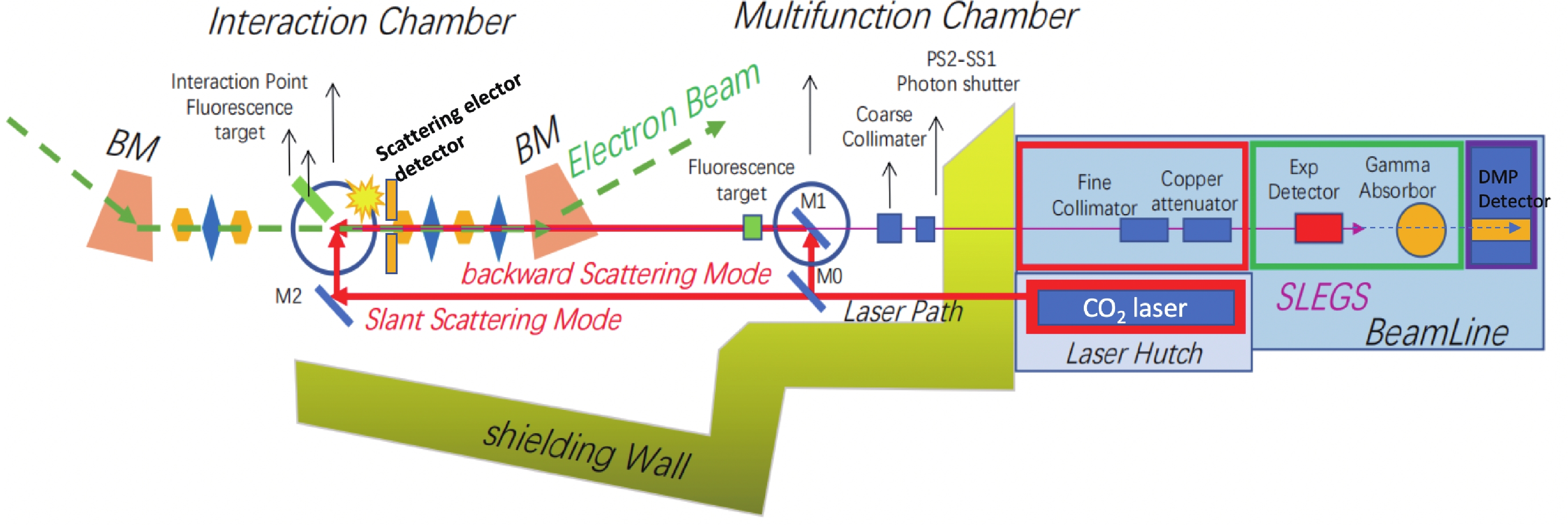Figure1. (color online) Scheme of the SLEGS (not to scale). 3.5 GeV electron pulses move in the storage ring. Photons from a CO₂ laser collide with electrons in two modes: in the line in which the colliding angle is $ 180^\circ $ and through a tunable colliding angle between $20^\circ$–$ 160^\circ $. Compton process products, including $ \gamma $-ray and the possible DMPs, are high concentrated at zero degrees (discussed in detail in the text) and are detected by DMP detectors in the experimental area. An electron detector is located around the target area to detect scattering electrons. It will serve as a start signal for the TOF of the possible DMPs, which will highly suppress background noise signals.

The Feynman diagrams for the LCS in the lowest order are shown in Fig. 2. For the SLEGS, if a low energy photon from the CO₂ laser is absorbed, a higher energy photon ($ \gamma $-ray) will be emitted, considering that the electron energy is 3.5 GeV. Similar to LCS processes, other rare processes related to DMP candidates may also occur when a photon collides with an electron. Instead of an actual $ \gamma $ photon, a pseudoscalar, scalar, or vector field particle, if it exists, will be emitted (Fig. 2). This is called a Compton-like process.
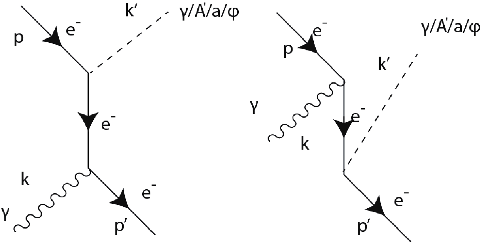Figure2. Feynman diagrams of Compton-like processes, which may produce a normal photon $ \gamma $ or DMPs. Here, the DMPs can be a dark photon $ A' $, axion a, or scalar particle $ \phi $. They can be generated via this Compton-like process between an actual photon and electron [15].

Here, we discuss different DMPs, such as pseudoscalar, vector, and scalar particles, that may be generated in Compton processes.
2

-->

A.Pseudoscalar particles

If pseudoscalar particles couple with electrons, the corresponding effective Lagrangian can be expressed as [22]

$ {\boldsymbol{L}} = g_{ae}\frac{\partial_\mu \phi_a}{2m_e}\bar{\psi}_e \gamma^\mu \gamma^5 \psi_e = -{\rm i} g_{ae}\bar{\psi}_e \gamma^5 \psi_e \phi_a, $

(1)

where the dimensionless $ g_{ae} $ is the pseudoscalar-electron coupling constant. Here, we consider a pseudoscalar particle that is emitted in a Compton-like process, i.e., $ \gamma+e^-\rightarrow e^- + a $. The corresponding Feynman diagram is shown in Fig. 2. The differential cross section can be expressed as

$ \begin{aligned}[b] \frac{{\rm d}\sigma}{{\rm d}\Omega} =& \frac{1}{64\pi^2}\frac{1}{E_k E_p |v_k-v_p|}\frac{|\vec{k'}|^2}{k'^0 p'^0} \\ &\times\left\vert\frac{1}{ \dfrac{\vert\vec{k'}|}{ k'^0}+\dfrac{|\vec{k'} |-(\vec{p}+\vec{k})\cdot \hat{k'}}{p'^0}}\right\vert\left(\frac{1}{2}\sum\limits_{\rm spin} |M^2|\right), \end{aligned}$

(2)

The definitions of $ \vec{k} $, $ \vec{k}' $, $ \vec{p} $, $ v_k $, $ v_p $, $ E_k $, $ E_p $, and M are provided in the Appendix. $ spin $ is the spin of the incoming electron.
Subsequently, the total cross section in the laboratory coordinator can be obtained by the integral

$ \begin{aligned}[b] \sigma_{\rm lab} = & \int {\rm d}\sigma = \prod\limits_f \left(\int \frac{{\rm d}^3 \vec{p}_f}{(2\pi)^3} \frac{1}{2E_f}\right) \frac{1}{2E_k 2E_p |v_k-v_p|} \\ &\times\left(\frac{1}{2}\sum\limits_{\rm spin} |M^2|\right)(2\pi)^4 \delta^4 (p+k-p'-k'), \end{aligned} $

(3)

where subscript index f is the final quantum state of the dark matter candidate (pseudoscalar particle) and electron.
Eq. (2) indicates that the differential cross section $\dfrac{{\rm d}\sigma_{\rm lab}}{{\rm d}\Omega}(m_a, \theta_0, \theta, \phi)$ is a function of the DMP mass $ m_a $, colliding angle between the electron and the laser $ \theta_0 $, and scattering angles, $ \theta $ and $ \phi $, whereas the total cross section $\sigma_{\rm lab}(m_a, \theta_0)$ depends only on $ m_a $ and $ \theta_0 $.
By using the parameters of SLEGS, $ E_e = 3.5 $ GeV and a photon wavelength of 10.64 $\mu$m, the cross section $\sigma_{\rm lab}(m_a, \theta_0)$ is shown in Fig. 3, which shows the results of four colliding angles: $ \theta_0 = 90^\circ $, $ 120^\circ $, $ 150^\circ $, and $ 180^\circ $. As the figure shows, at $ \theta_0 = 180^\circ $, i.e., head-to-head collision, the cross section approaches its maximum. Moreover, the cross section decreases as the mass of the pseudoscalar particle increases. The differential cross section $\dfrac{{\rm d}\sigma_{\rm lab}}{{\rm d}\Omega}(m_a, \theta_0, \theta, \phi)$ is provided in the Appendix.
Figure3. (color online) Cross sections of the pseudoscalar particle through the reaction $ e+\gamma \rightarrow e+a $. The cross section $\sigma_{\rm lab}(m_a, \theta_0)$ is a function of the pseudoscalar particle mass $ m_a $, and colliding angle $ \theta_0 $ between the pseudoscalar particle and electron. The different color lines represent $ \theta_0 = 90^\circ $ (blue dash dot dot), $ 120^\circ $(green dash dot), $ 150^\circ $(red dash), and $ 180^\circ $(black solid). The cross section $ \sigma $ is in barns.

2 -->

B.Dark photon

For the coupling of vector field particles, such as dark photons, to an electron, the corresponding effective Lagrangian can be expressed as [7]

$ {\boldsymbol{L}} = g_{A'e} e \bar{\psi}_e \gamma^\mu \psi_e A'_\mu, $

(4)

where the dimensionless $ g_{A'e} $ is the mixing parameter between the dark photon and the Standard Model photon, and e is the electron charge. Similar to the Compton process, the dark-photon-electron interaction process can be expressed as $ \gamma+e^-\rightarrow e^- + A' $. The corresponding Feynman diagram is shown in Fig. 2.
The differential and total cross sections of the interaction are described in detail in the Appendix. Similar to the pseudoscalar particle scenario, with an electron energy of $ E_e = 3.5 $ GeV and the laser polarization direction perpendicular to the reaction plane, the cross section $\sigma_{\rm lab}(m_a, \theta_0)$ for interaction $ \gamma+e^-\rightarrow e^- + A' $ is shown in Fig. 4, which shows the $\sigma_{\rm lab}(m_a, \theta_0)$ values at colliding angles of $ \theta_0 = 90^\circ $, $ 120^\circ $, $ 150^\circ $, and $ 180^\circ $. Again, the head-to-head collision at $ \theta_0 = 180^\circ $ has the maximum cross section compared with other collision angles. The cross section for the dark photon decreases as its mass increases. The dependence of the differential cross section on scattering angles with the dark photon is discussed in the Appendix.
Figure4. (color online) Cross sections of dark photons through the reaction $ e+\gamma \rightarrow e+\phi $. The cross section $\sigma_{\rm lab}(m_a, \theta_0)$ is a function of the dark photon mass $ m_{A'} $, and colliding angle $ \theta_0 $ between dark photon and electron. The different color lines represent $ \theta_0 = 90^\circ $ (blue dash dot dot), $ 120^\circ $(green dash dot), $ 150^\circ $(red dash), and $ 180^\circ $(black solid). The cross section $ \sigma $ is in barns.

2 -->

C.Scalar dark matter particle

For a scalar DMP, $ \gamma+e^-\rightarrow e^- + \phi $, the corresponding effective Lagrangian can be expressed as [23]

$ L = g_{\phi e} \bar{\psi}_e \psi_e \phi, $

(5)

where the dimensionless $ g_{\phi e} $ is the scalar-field-particle-electron coupling constant. The corresponding Feynman diagram is shown in Fig. 5.
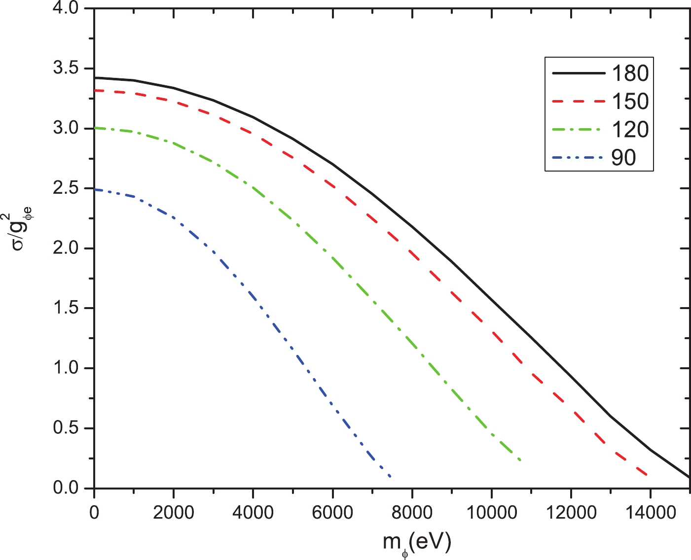Figure5. (color online) Scalar DMP generating cross sections through the reaction $ e+\gamma \rightarrow e+\phi $. The cross section $\sigma_{\rm lab}(m_a, \theta_0)$ is a function of scalar DMP mass $ m_\phi $, and colliding angle $ \theta_0 $ between the scalar DMP and electron. The different color lines represent $ 180^\circ $ (black solid), $ 150^\circ $ (red dash), $ 120^\circ $ (green dash dot), and $ \theta_0 = 90^\circ $ (blue dash dot dot). The cross section $ \sigma $ is in barns.

Using an electron energy of $ E_e = 3.5 $ GeV, the cross section $\sigma_{\rm lab}(m_a, \theta_0)$ for interaction $ \gamma+e^-\rightarrow e^- + \phi $ can be calculated, and shown in Fig. 5, for the scattering angles $ \theta_0 = 90^\circ $, $ 120^\circ $, $ 150^\circ $, and $ 180^\circ $. For the same mass of a scalar DMP, the interaction cross section increases with increasing scattering angle and reaches its maximum at $ \theta_0 = 180^\circ $. For detection at other given angles, the expected cross section decreases as the scalar DMP mass increases.
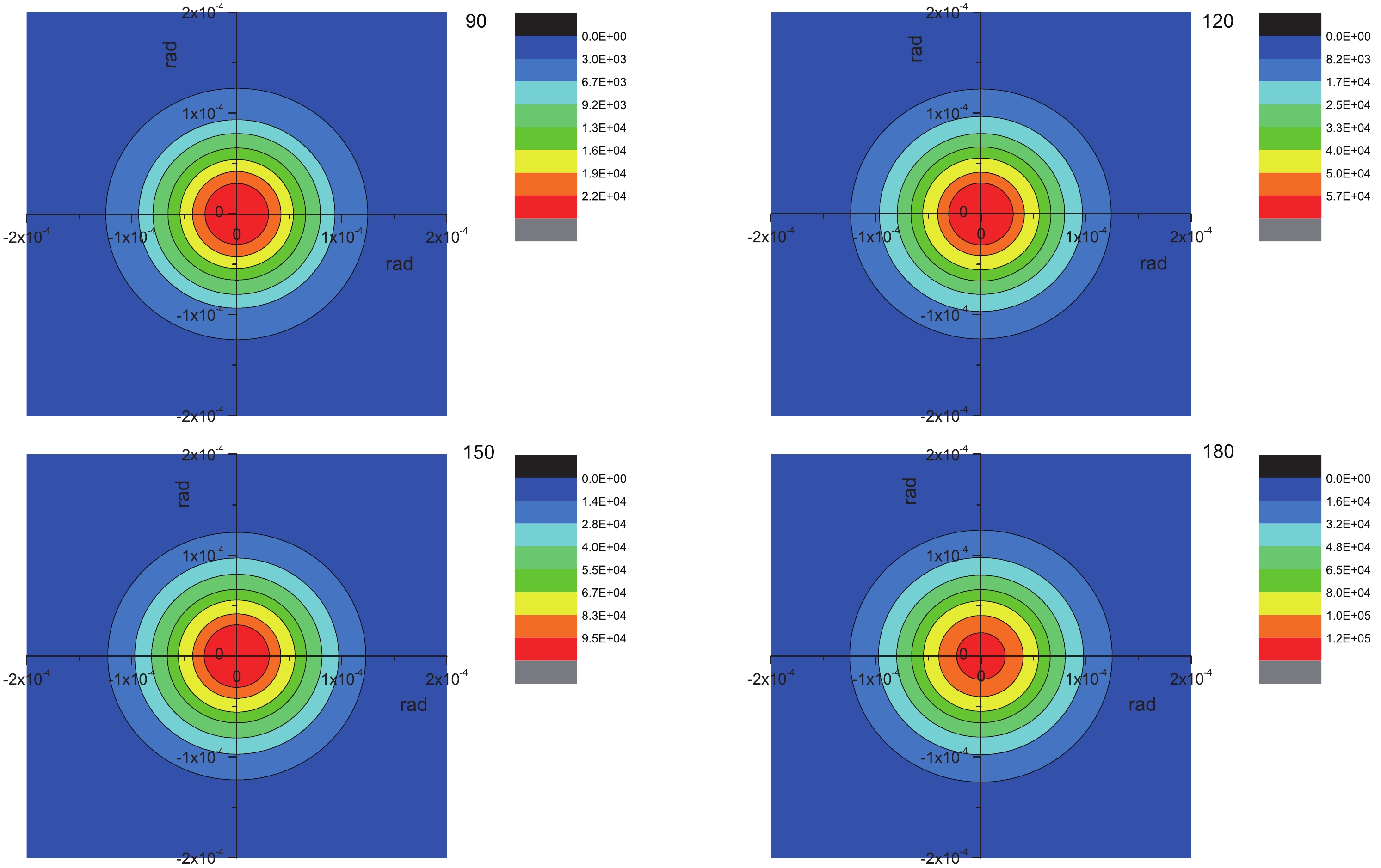
Further information on the interaction's differential and total cross sections are described in the Appendix, from which we observe that the cross sections have different dependences on the scattering angles. In the calculations, the polarization of the laser beam is parallel to the y-axis. The cross section of pseudoscalar particles is insensitive to the polarization of the incoming photon (Fig. A1). However, the cross sections of dark photons and scalar particles are highly dependent on the polarization of the laser beam (Fig. B1 & C1). The dark photons are primarily emitted parallel to the x-direction, which is similar to the Thomson scattering. In contrast, the scalar particles are emitted primarily parallel to the y-direction (Fig. C1). This is because the radiation of scalar particles is parallel to the laser’s polarization. The angular distributions can be used to distinguish different types of dark matter candidates since the distributions highly depend on particle types.
FigureA1. (color online) Differential cross sections of pseudoscalar particles through the reaction $ e^-+\gamma \rightarrow e^-+a $. The mass is selected to be $ 0 $. The origin represents the z-direction. The exit angle $ \theta $ of the DMP is represented by $ \sqrt{x^2+y^2} $. The unit is $ barn/(g^2_{ae}\cdot sr^2) $.

FigureB1. (color online) Cross sections of dark photons through the reaction $ e+\gamma \rightarrow e+A' $. The mass is selected to be $ 0 $. The origin represents the z-direction. The exit angle $ \theta $ of the DMP is represented by $ \sqrt{x^2+y^2} $. The unit is $ barn/(g^2_{A'e}\cdot sr^2)$.

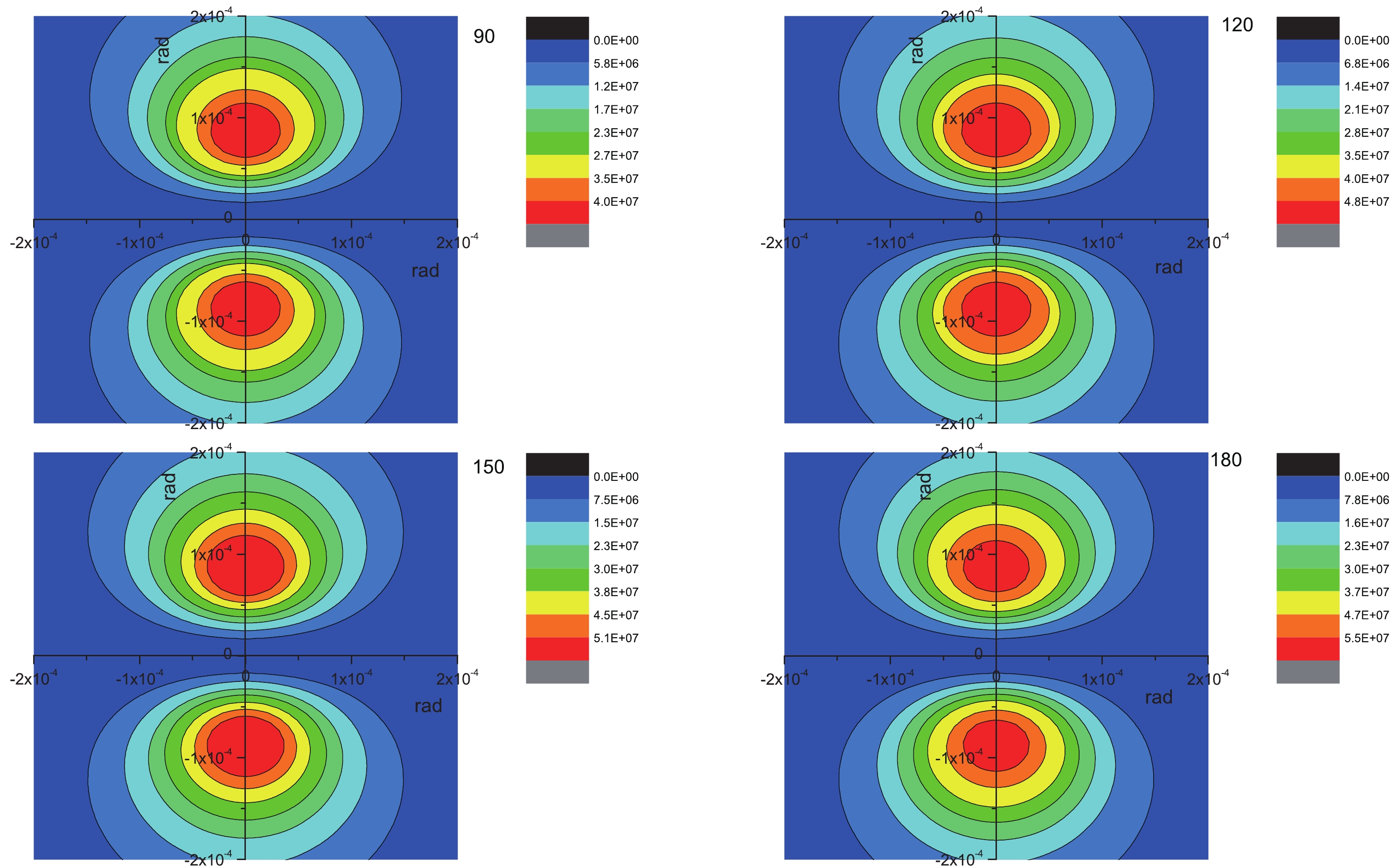FigureC1. (color online) Cross sections of scalar particles through the reaction $ e+\gamma \rightarrow e+\phi $. The mass is chosen to be $ 0 $. The origin represents the z-direction. The exit angle $ \theta $ of the DMPs represented by $ \sqrt{x^2+y^2} $. The unit is $ barn/(g^2_{\phi e}\cdot sr^2) $.

DMPs may be detected by placing a detector set in the experimental area and an electron detector set near the target, as shown in Fig. 6 (also in Fig. 1). After the laser-electron collision, scattered electrons can be detected by the electron detector set, while the $ \gamma $-photons, or the DMPs, will be emitted in a narrow forward solid angle (Fig. A1-C1 in the Appendix). The $ \gamma $-photons will be absorbed by the $ \gamma $-blocker, and the possible DMPs passing through the $ \gamma $-blocker can be recorded by the DMP detector through the reaction $ X+e\rightarrow e+\gamma $.
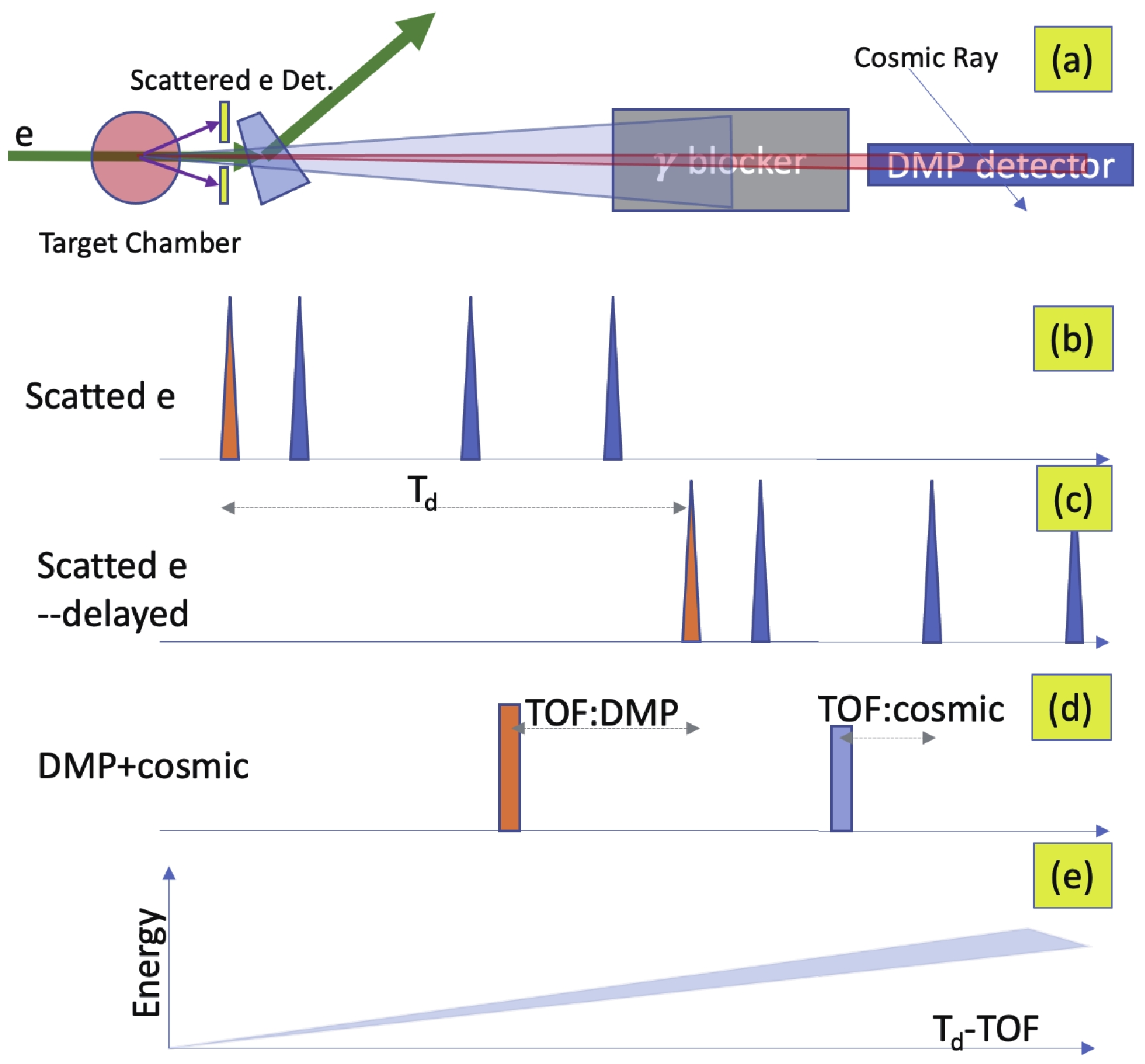Figure6. (color online) Inverse-TOF method for the possible DMPs. (a) Detecting scheme for the possible DMPs. The $ \gamma $ photons are stopped by the $ \gamma $-blocker, the possible DMPs are detected by the DMP detector through the reaction $ X+e\rightarrow e+\gamma $, and the scatted electrons from the inverse Compton scattering are detected by a detector array. (b) Signals ($ S_e $) recorded by the electron detector array. (c) Delayed signals ($ S^{(d)}_e $) of ($ S_e $). The delay time is $ T_d $. (d) Signals from the DMP detectors, including these from the possible DMPs, cosmic rays, and/or other ambient radiations. (e) Energy vs. $(T_d-{\rm TOF})$ spectrum, where the shaded area represents signals from DMPs that have relatively high energies (MeV) and low rest mass (keV).

Because the rate of the scatted electron is significantly larger than that of DMPs, an inverse-TOF method can be used to determine the TOF of possible DMPs (Fig. 6(b)-(d)). A signal from the DMP detector is used as the “start” of the TOF, while delayed signals from the electron detector set are used as the “stop.” With this method, the rate of the TOF of the DMP is highly reduced, which results in a large decrease in the random coincidence rate. In the energy vs. TOF spectrum, the to-be-discovered DMP signals are located in a very narrow area because of their high energy (MeV) and low rest mass (keV). The DMP detector can also record background signals such as ambient radiation and cosmic rays. Because the background signals are random, this type of data is randomly distributed in the TOF vs. energy spectrum, and only a very few of them fill the region of interest. Furthermore, the cosmic rays and ambient radiations can be further reduced using an anti-cosmic-muon device and passive shielding.
The time and energy resolutions of the DMP detector determine the rejection rate for the random background signals. With modern detecting technologies, a TOF precision of approximately tens of ps, as well as energy resolution of less than 1%, can be achieved.
The inverse-TOF method can only operate with a well-defined electron beam structure. A typical electron beam structure is shown in Fig. 7. The linear accelerator can operate in two modes: single bunch or multi-bunch [21]. Each bunch has a sub-ns width. The time interval between two bunches is 2 ns. In the multi-bunch mode, many single bunches can be combined into a macro pulse. For example, as shown in Fig. 7, a macro pulse with 120 bunches has a width of 240 ns, followed by 80 ns (40 periods) of silence time, and the pattern is repeated. Therefore, the well-defined electron beam structure provides a good initial point for the DMP data analysis.
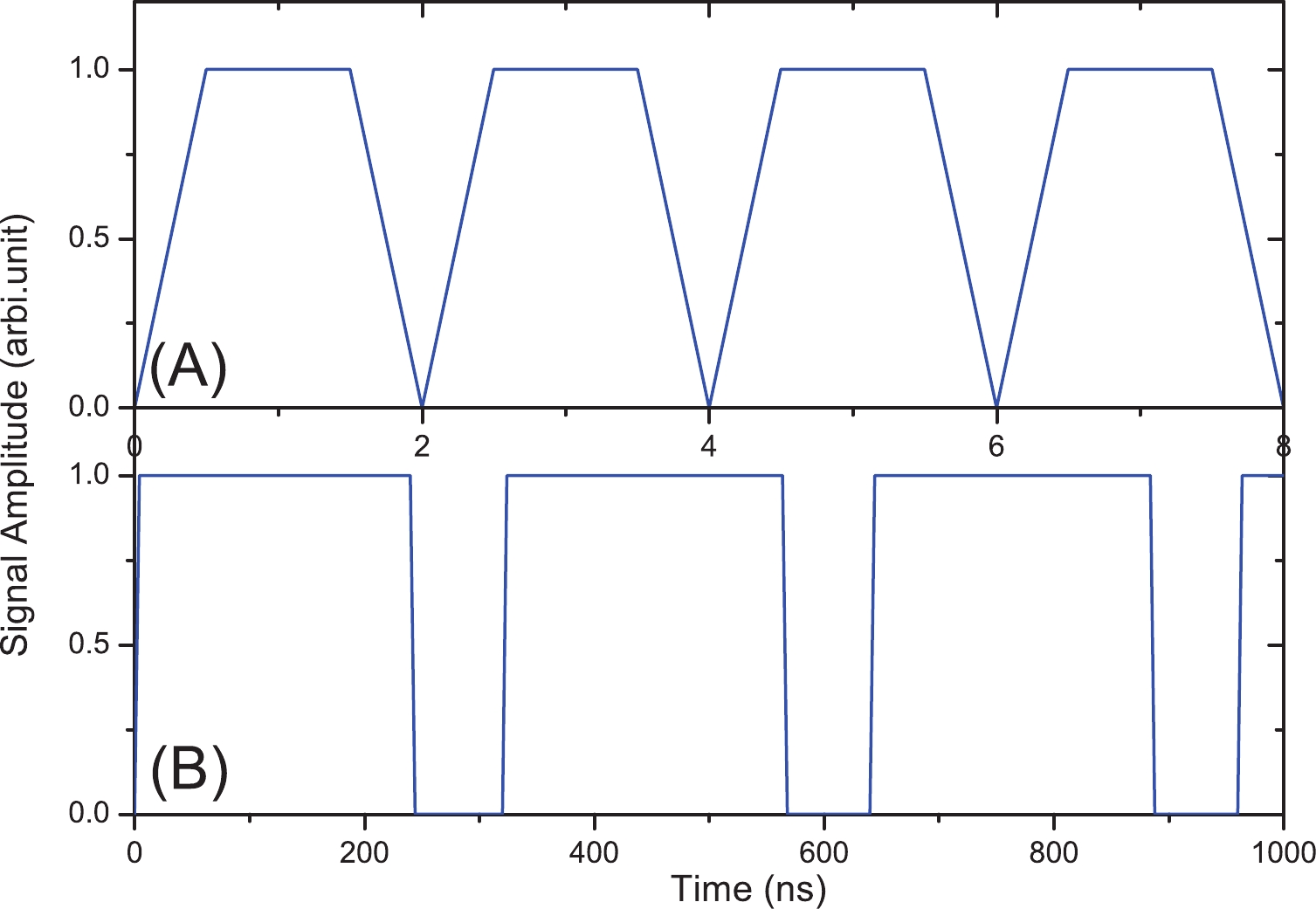Figure7. (color online) Schematic diagram of a typical electron beam structure at SSRF. The electron beam is composed of small bunches with widths smaller than 1 ns [21]. Multiple bunches can be combined into a macro pulse. (A) Zoomed-in structure of the beam in time range 0 to 8 ns; (B) zoomed-out structure in range 0 to 1000 ns. A macro pulse with 120 single bunches has a width of 240 ns.

With assumptions of a continuous-wave laser with a power of 1000 kW, a laser focus diameter of 2 $\mu$m, an electron beam energy of 3 GeV, an electron beam intensity of 240 mA, a time resolution of the TOF 0.1 ns, a detector length of 30 m, and two years of data collecting time, the DMP detecting rates were simulated. The results of the constraints on pseudoscalar, dark photon, and scalar particles are shown in Figs. 8-10.
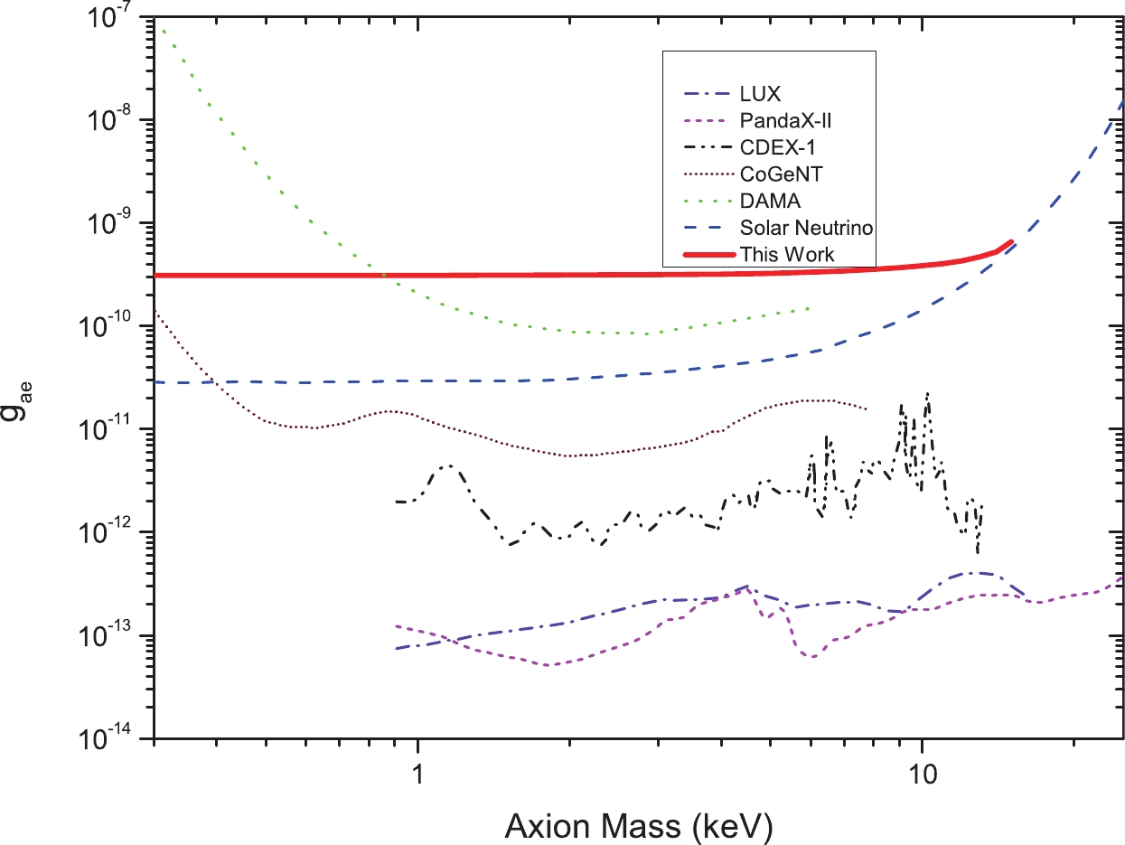Figure8. (color online) Pseudoscalar-electron coupling limits. The lines in the figure represent limits from LUX (purple dash dot) [27], PandaX-II (pink dash) [28], CDEX-1 (black dash dot dot) [29], CoGeNT (brown dot) [30], DAMA (green short dash) [31], solar neutrino [32] (blue dash), and this study (red solid) with a pulse laser with a peak power of 1000 kW and two years of data collecting.

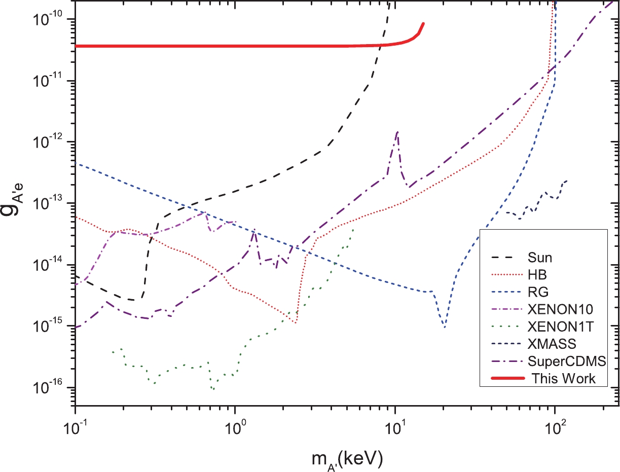Figure9. (color online) Electron-dark-photon coupling limits. The lines in the figure represent limits from the Sun (black dash) [33], horizontal branch stars (HB, pink dot) [33], red giant (RG, blue short dash) [33], XENON10 (pink dash dot) and XENON1T (green dot) [33], XMASS (black short dash) [34], SuperCDMS (purple dash dot) [35], and this study (red solid) with a pulse laser with a peak power of 1000 kW and two years of data collecting.

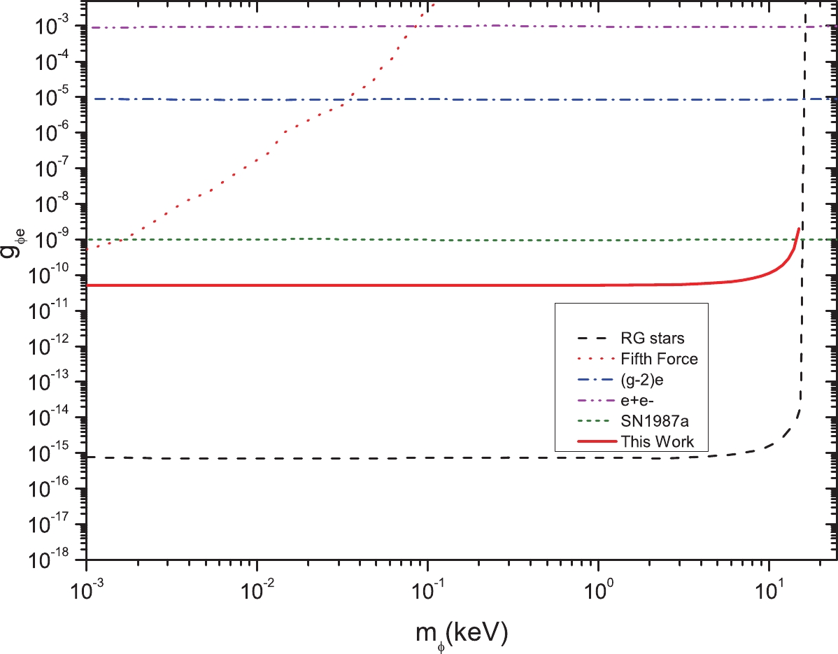Figure10. (color online) Electron-scalar-DMP coupling limits. The x-axis $ m_\phi $ represents the rest mass of the scalar DMP. The lines in the figure represent limits from red giant stars (black dash) [23, 36], fifth force searches (orange dot) [23, 37], electron g-2 (blue dash dot) [23, 38], $ \phi\rightarrow e^+e^- $ (pink dash dot dot) [23, 38], supernova SN1987a (green short dash) [36], and this study (red solid) with a pulse laser with a peak power of 1000 kW and two years of data collecting.

A pulsed laser can be used to further improve the constraints on the DMP coupling constants. The peak power of a pulsed laser could be in the range of several GW to even TW with today's technologies. As the laser peak power $ P_{L} $ increases, the constraints on the DMP coupling constants can be reduced using $ \propto P_{L}^{1/2} $. By adding an optical cavity, the constraints may be improved by a factor of over 1000 [24, 25].
There is another advantage. When SLEGS is operating, it does not interfere with other ongoing experiments at the SSRF. Furthermore, DMP experiments do not interfere with $ \gamma $-ray experiments that are also ongoing on the SLEGS. A DMP experiment will be silent. Whenever the facility is operating, it records data.
Another electron facility, Shanghai HIgh repetitioN rate XFEL aNd Extreme light facility (SHINE) [26], is under construction in the Shanghai area. It will have energy up to 8.8 GeV, 100 pC/bunch, and a repeating frequency of 1 MHz, making it feasible for DMP search experiments.

In this paper, the possibilities of searching for dark matter particles using the SLEGS beamline are discussed. An advantage of using electron-photon Compton scattering to search for DMPs is that the scattered DMPs are highly concentrated in forwarding angles, which makes their detection easier. Through the use of electron detectors as start signals of the TOF, the background noise, which is the key problem in the detection of extremely rare events, can be highly suppressed. Electron facilities are promising platforms for the search of light DMPs such as axions, dark photons, and dark scalar particles.

The scattering cross section can be obtained directly from an S-matrix.

$\tag{A1} \begin{aligned}[b]\frac{{\rm d}\sigma}{{\rm d}\Omega} =& \frac{1}{64\pi^2}\frac{1}{E_k E_p |v_k-v_p|}\frac{|\vec{k'}|^2}{k'^0 p'^0} \\&\times\left\vert\frac{1}{ \dfrac{\vert\vec{k'}|}{ k'^0}+\dfrac{|\vec{k'} |-(\vec{p}+\vec{k})\cdot \hat{k'}}{p'^0}}\right\vert\left(\frac{1}{2}\sum |M^2|\right), \end{aligned} $

(A1)

$ \tag{A2}\begin{aligned}[b] {\rm d}\sigma =& \frac{1}{2E_k 2E_p |v_k-v_p|} \left( \prod\limits_f \frac{{\rm d}^3 p_f}{(2\pi)^3} \frac{1}{2E_f} \right)\\&\times\left(\frac{1}{2}\sum\limits_{\rm spin} |M^2|\right)(2\pi)^4 \delta^4 (p+k-p'-k'), \end{aligned}$

where we replace $ |M|^2 $ with $\dfrac{1}{2}\displaystyle\sum_{\rm spin}|M|^2$ because the electron's spin is not controllable. It is the average of all possible electron spins. The z-axis is selected to be the moving direction of the incoming electron. The photon and electron are located in the x-z plane. The four momenta of all particles in the Cartesian coordinates are $ p = $$ (p^0,0,0,|\vec{p}|) $, $ k = (k^0,|\vec{k}|\sin\theta_p,0,|\vec{k}|\cos\theta_p) $, and $ k' = (k'^0, |\vec{k'}) $$ |\sin\theta \cos\phi, |\vec{k'})|\sin\theta \sin\phi|,\vec{k'})|\cos\theta ) $. The four momenta of the emitted particles, $ p' $ and $ k' $, can be determined by solving the energy momentum conservation and energy momentum relation: $ p^2 = p'^2 = m_e^2 $ and $ k'^2 = m_A^2 $.
For different types of particles (pseudoscalar, scalar, and vector), $\dfrac{1}{2}\displaystyle\sum_{\rm spin}|M|^2$ can be expressed as follows.
2

-->

A.Pseudoscalar particles

There are two possible Feynman diagrams for the interaction $ e^- \gamma \rightarrow e^- \psi_a $, Fig. 2. For a pseudoscalar particle, $\dfrac{1}{2}\displaystyle\sum_{\rm spin}|M|^2$ is

$\tag{A3}\begin{aligned}[b] \frac{1}{2}\sum\limits_{\rm spin}|M|^2 =& -g_{ae}^2 e^2 \left(\frac{I}{\Big((p+k)^2-m_e^2\Big)^2} \right.\\&+\frac{II}{\Big((p+k)^2-m_e^2\Big) \Big((p-k')^2-m_e^2\Big)} \\&\left.+\frac{III}{\Big((p-k')^2-m_e^2\Big)^2}\right), \end{aligned}$

The nominators are

$\tag{A4} \begin{aligned}[b] I =& 4(p'\cdot k)(k \cdot p)+8( p'\cdot k)( p \cdot \epsilon) (p \cdot \epsilon)\\&-8( p'\cdot \epsilon)( k\cdot p)(p \cdot \epsilon)+8( p'\cdot p)( p\cdot \epsilon)( p\cdot \epsilon)\\&-8m_e^2 ( p\cdot \epsilon)( p\cdot \epsilon), \end{aligned} $

$ \tag{A5}\begin{aligned}[b] \frac{II}{2} = &4(p \cdot k)(p' \cdot k)+4( p'\cdot \epsilon)( p'\cdot k)(p \cdot \epsilon )\\&-4(p' \cdot \epsilon )(p' \cdot \epsilon)( p\cdot k)+4(p \cdot \epsilon)( p'\cdot k)( p\cdot \epsilon)\\&-4( p\cdot \epsilon)(p' \cdot \epsilon)( p\cdot k)\\&+8( p\cdot \epsilon)(p' \cdot \epsilon)(p' \cdot p)-8m_e^2 ( p\cdot\epsilon )( p'\cdot \epsilon), \end{aligned} $

$\tag{A6}\begin{aligned}[b] III =& 4(p \cdot k)(p' \cdot k)-8(p' \cdot \epsilon )(p' \cdot \epsilon )( k\cdot p)\\&+8( p'\cdot \epsilon)( p'\cdot k)( p\cdot \epsilon)+8( p'\cdot p)(p' \cdot \epsilon)(p' \cdot \epsilon)\\&-8m_e^2 ( p'\cdot \epsilon)( p'\cdot \epsilon), \end{aligned} $

where $ \epsilon $ is the polarization direction of the photon. Here, it points in the y-direction. The differential cross section at different collision angles ($ \theta = 90^\circ, 120^\circ, 150^\circ $, and $ 180^\circ $) are shown in Fig. A1. As expected, because the energy of the electron is significantly larger than that of the photon, in the laboratory frame, the expected scalar DMPs are highly concentrated in the forward angle. This property will benefit experimental detection.
2 -->

B.Dark photon

Similar to the pseudoscalar scenario, the $\dfrac{1}{2}\displaystyle\sum_{\rm spin}|M|^2$ of the vector particle (dark photon) can be expressed as

$ \tag{B1}\begin{aligned}[b] {\rm i}M =& \bar{u}(p') (-{\rm i} g_{A'e}\epsilon^*_\nu(k') \gamma^\nu )\frac{{\rm i}({\not\!\! p}+{\not\! k}+m_e)}{(p+k)^2-m_e^2} \\&\times(-{\rm i}e\epsilon_\mu(k)\gamma^\mu)u(p)\\&+\bar{u}(p')(-{\rm i}e\epsilon_\mu(k)\gamma^\mu) \frac{{\rm i}({\not\!\! p}-{\not\! k}'+m_e)}{(p-k')^2-m_e^2} \\&\times(-{\rm i} g_{A' e} \epsilon^*_\nu(k') \gamma^\nu )u(p), \end{aligned} $

where $ \epsilon_\nu $ is the polarization direction of the photon. Here, it points in the y-direction. The nominators are

$\tag{B2} \begin{aligned}[b] I =& 8(p'\cdot k)(p\cdot k)-16( p\cdot k)(p' \cdot \epsilon)( p\cdot \epsilon)\\&+16( p'\cdot k)( p\cdot \epsilon)( p\cdot \epsilon)\\&+16( p'\cdot p)( p\cdot \epsilon)( p\cdot \epsilon)-32m_e^2 ( p\cdot \epsilon )( p\cdot \epsilon), \end{aligned} $

$\tag{B3}\begin{aligned}[b] \frac{II}{2} =& -8( p'\cdot \epsilon)( k\cdot p)( p\cdot \epsilon)+8( p'\cdot k)( p\cdot \epsilon)( p\cdot \epsilon)\\&+8( p'\cdot k)( p\cdot \epsilon)( p'\cdot \epsilon)-8( p'\cdot \epsilon)( k\cdot p)(p' \cdot \epsilon)\\& +16( p'\cdot p)(p' \cdot \epsilon)( p\cdot \epsilon)-32m_e^2(p' \cdot \epsilon)( p\cdot \epsilon), \end{aligned} $

$ \tag{B4}\begin{aligned}[b] III =& 8(p' \cdot k)( p\cdot k)-16(k \cdot p)(p' \cdot \epsilon)( p'\cdot \epsilon)\\&+16( p'\cdot k)(p \cdot \epsilon)( p'\cdot \epsilon)+16( p'\cdot p)( p'\cdot \epsilon)( p'\cdot \epsilon)\\& -32m_e^2 ( p'\cdot \epsilon). \end{aligned} $

The differential cross section at different collision angles ($ \theta = 90^\circ, 120^\circ, 150^\circ $, and $ 180^\circ $) are shown in Fig. B1. As expected, because the energy of the electron is significantly larger than that of the photon, in the laboratory frame, the expected scalar DMPs are highly concentrated in the forward angle. This property will benefit experimental detection.
2 -->

C.Scalar

Similar to the pseudoscalar scenario, the $\dfrac{1}{2}\displaystyle\sum_{\rm spin}|M|^2$ of the scalar particles can be expressed as

$\tag{C1}\begin{aligned}[b] {\rm i}M = &\bar{u}(p') (-{\rm i} g_{\phi e} )\frac{{\rm i}({\not\!\! p}+{\not\! k}+m_e)}{(p+k)^2-m_e^2}\\&\times (-{\rm i}e\epsilon_\mu(k)\gamma^\mu)u(p)\\&+\bar{u}(p')(-{\rm i}e\epsilon_\mu(k)\gamma^\mu)\\&\times \frac{{\rm i}({\not\!\!p}-{\not\! k}'+m_e)}{(p-k')^2-m_e^2} (-{\rm i} g_a )u(p), \end{aligned}$

Here, it points in the y-direction. The nominators are

$\tag{C2}\begin{aligned}[b] I =& 4( p'\cdot k)( p\cdot k)+8( p\cdot \epsilon)( p'\cdot k)(\epsilon \cdot p)\\&-8( p\cdot \epsilon)( p'\cdot \epsilon)( p\cdot k)\\&+8(p \cdot \epsilon)( p\cdot \epsilon)( p'\cdot p)\\&+8m_e^2( p\cdot \epsilon)( p\cdot\epsilon ), \end{aligned} $

$\tag{C3}\begin{aligned}[b] \frac{II}{2} =& 4( p'\cdot k)( k\cdot p)-4(p \cdot \epsilon)( p'\cdot \epsilon)( k\cdot p)\\&+4( p\cdot \epsilon)( p'\cdot k)(p \cdot \epsilon)-4( p'\cdot \epsilon)(p' \cdot \epsilon)(p \cdot k)\\& +8( p'\cdot p)(p' \cdot \epsilon)( p\cdot \epsilon)+8m_e^2(p' \cdot \epsilon)(p \cdot \epsilon), \\&+4(p' \cdot \epsilon)( p'\cdot k)(p \cdot \epsilon) \end{aligned} $

$ \tag{C4}\begin{aligned}[b] III =& 4(p \cdot k)( p'\cdot k)-8( p'\cdot\epsilon )( p'\cdot \epsilon)( k\cdot p)\\&+8(p' \cdot \epsilon)( p'\cdot k)( p\cdot \epsilon)+8( p'\cdot \epsilon)( p'\cdot \epsilon)( p'\cdot p)\\&+8m_e^2 (p' \cdot \epsilon)(p' \cdot \epsilon), \end{aligned} $

where $ \epsilon $ is the polarization direction of the photon. The differential cross section at different collision angles ($ \theta = 90^\circ, 120^\circ, 150^\circ $, and $ 180^\circ $) are shown in Fig. C1. As expected, because the energy of the electron is significantly larger than that of the photon, in the laboratory frame, the expected scalar particles are highly concentrated in the forward angle. This property will benefit experimental detection.