A. Soylu ^1,
, F. Koyuncu ^2,
, G. Gangopadhyay ^3,
, V. Dehghani ^4,
, S. A. Alavi ^4,
, 1.Department of Physics, Nigde ?mer Halisdemir University, Nigde 51240, Turkey
2.Program of Opticianry, G?lhisar Vocational School of Health Services, Burdur Mehmet Akif Ersoy University, 15400, G?lhisar, Burdur, Turkey
3.Department of Physics, University of Calcutta, Kolkata 700009, India
4.Department of Physics, University of Sistan and Baluchestan, Zahedan, Iran
Received Date:2020-10-07
Available Online:2021-04-15
Abstract:The dependence of proton emission half-lives on the nuclear asymmetry parameter is investigated using the WKB method and two types of empirical formula. Using the single-folding formalism with asymmetry-dependent nuclear radius and surface diffuseness of nuclear matter, the nuclear potential and consequently the half-life are functions of the asymmetry factor. Despite small values of asymmetry in neutron-deficient proton emitters, noticeable changes in the half-lives are observed. The addition of an asymmetry parameter term to the two forms of empirical formulas leads to a reduction in the rms error for ground state and isomeric transitions. A noticeable reduction of about 43% is obtained for isomeric transitions in the second form of the empirical formula. Considering ground state transitions in two categories, odd-even and odd-odd emitters, and adopting deformation and asymmetry-dependent empirical formulas, the rms decreases remarkably. The lowest values of rms errors, viz. 0.1492, 0.2312, and 0.1999, are obtained for the aforementioned empirical formulas for ground state transitions of odd-even and odd-odd emitters and for all isomeric transitions, respectively.

HTML

--> --> -->

Proton emission is an interesting and relatively recent topic in the study of nuclear decay. Finding proton emission half-lives may be of great importance in understanding the decay features of nuclei [1], determining nuclear deformation, studying the behavior of single-particle resonances close to the drip line [2], constraining the density slope of the symmetry energy [3], and understanding the termination of the astrophysical rp-process [4]. Very informative introductions to the history of proton emission, experimental techniques and methods, and theories of proton emission have been provided in a number of review papers [5-9].
The nuclear deformation and the asymmetry parameter are two important properties in the study of nuclear decay. In different theoretical models for the calculation of proton emission half-lives, the nuclear deformation has been included directly through explicit dependence on the Coulomb and nuclear potentials [10-13]. Moreover, the nuclear asymmetry parameter has been included in the nuclear potential and spectroscopic factor [14-17]. The proton emission empirical formula is basically a function of the Q-value of proton emission and the atomic number of the daughter nucleus. The formula may comprise the nuclear properties of parent or daughter nuclei, such as orbital angular momentum and deformation parameters, through microscopic foundations or the introduction of new modification terms. The dependence of the empirical half-life on these additional terms may be justified based on microscopic or macroscopic theoretical calculations. The first empirical formula in this regard introduced an implicit function of deformation and momenta [1]. An empirical formula as a function of deformation has been given in Ref. [18]. The effects of deformation and Q-value on empirical formulae have been investigated in our previous work [19]. This motivated us to assess the effect of deformation and the asymmetry parameter, separately as well as together, on two forms of empirical formula. Using the single-folding potential [20, 21] and adopting asymmetry parameter dependent densities, the influence of the asymmetry parameter on calculated half-lives can be evaluated.
In Sec. II, the theory related to our calculations is given in two parts, theoretical calculations and empirical formulas. The results of our calculation are given in Sec. III. Finally, the conclusion and summary are presented in Sec. IV.

In order to show the dependence of the theoretical half-life on the asymmetry parameter, this section is divided into two parts: theoretical half-life and empirical half-life.
2

-->

A.Theoretical half-life

The effective interaction potential between a proton and daughter nucleus, $ V_{\rm eff} $(r), includes the attractive nuclear potential $ V_N(r) $, the repulsive Coulomb potential $ V_{\rm C}(r) $, and the repulsive centrifugal term $ V_l(r) $

$ V_{\rm eff}(r) = V_N(r)+V_{\rm C}(r)+V_l(r), $

(1)

where r is the relative distance between the proton and the daughter nucleus and l is the angular momentum carried by the proton.
The nuclear potential can be calculated through the single folding model,

$ V_{N}(r) = \int {\rm d}\vec{r}_1 \rho(\vec{r}_1) v(s) , $

(2)

where $ s = |\vec{r}_1-\vec{r}| $ is the relative distance between interacting nucleon pairs. The effective nucleon-nucleon potential Yukawa (M3Y)-Reid-type interaction with zero-range exchange contribution is given by [22]

$ v(s) = 7999 \frac{{\rm e}^{-4s}}{4s}-2134 \frac{{\rm e}^{-2.5s}}{2.5s}-276\delta(s). $

(3)

Here, $ \rho(\vec{r}_1) $ is the matter density distribution of the daughter nucleus, which is given by the two-parameter Fermi distribution:

$ \rho(r) = \frac{\rho_0}{1+\exp\left[\dfrac{r-R}{a}\right]}. $

(4)

The radii and surface diffuseness parameters used are $ R = 1.07 A^{1/3} ({\rm fm}) $ and $ a = 0.54\; ({\rm fm}) $ [23]. We use the following asymmetry parameter dependent formulas for proton and neutron radii, $ R_p $ and $ R_n $, and corresponding surface diffuseness $ a_p $ and $ a_n $ [24],

$ \begin{aligned}[b]&R_p = 1.249 A^{1/3}-0.5401-0.9582\; I,\\&R_n = 1.2131 A^{1/3}-0.4415+0.8931 \; I,\\&a_p = 0.4899-0.1236 \;I,\\& a_n = 0.4686+0.0741 \; I,\end{aligned} $

(5)

where $I = \dfrac{N-Z}{A}$ is the asymmetry parameter of the daughter nucleus. Two separate asymmetry-dependent proton and neutron matter density distributions, $ \rho_p $ and $ \rho_n $, are obtained and consequently the nuclear potential is obtained as

$ V_N(r) = V^n_N(r)+V^p_N(r) = \int {\rm d}\vec{r}_1 \rho_n(\vec{r}_1) v(s)+\int {\rm d}\vec{r}_1 \rho_p(\vec{r}_1) v(s), $

(6)

where $ V^n_N $ and $ V^p_N $ are the contributions of the neutron and proton to the total nuclear potential. As for the different proton and neutron density distributions and the introduction of the asymmetry term in the folding potential, there have already been quite a few studies of alpha or heavier cluster decay [25, 26].
The Coulomb potential $ V_{\rm C}(r) $ is determined through the single-folding potential Eq. (2) by replacing the matter distribution with charge distribution and the M3Y nucleon-nucleon potential with a repulsive proton-proton potential $v(s) = \dfrac{e^2}{4\pi\epsilon_0}\dfrac{1}{s}$.
The proton emission half-life can be calculated through the WKB approximation. The two necessary conditions of the WKB for the centrifugal term and nuclear potential, respectively, are the Langer modification and Bohr$ - $Sommerfeld quantization condition [27]. So, the effective potential with these modifications is written as

$ V_{\rm eff}(r) = \eta V_N(r)+ V_{\rm C}(r)+\dfrac{\hbar^2\left(l+\dfrac{1}{2}\right)^2}{2\mu r^2} ,$

where $ \eta $ is the quantization factor.
In Ref. [28] the asymmetry dependence of the nuclear potential has been investigated by adding the Lane potential [29] to the nuclear potential $ V_N(r)+V_N^{\rm Lane}(r) $. The Lane nuclear potential can be approximately written as $V_N^{\rm Lane}(r) = -I_d \dfrac{V_N(r)}{2}$ [30]. Therefore, the total nuclear potential is obtained as $\left(1- \dfrac{I_d}{2}\right)V_N(r)$, and the asymmetry appears in the coefficient of the nuclear potential. Hence, by considering the quantization condition the asymmetry dependence is eliminated.
The proton emission half-life is calculated as

$ T_{1/2} = \frac{\ln 2}{\nu P S_p}, $

(7)

where $ \nu $, P, $ S_p $ are the assault frequency, tunneling probability, and spectroscopic factor, respectively. Using the WKB approximation, the assault frequency and tunneling probability are given as

$ \begin{aligned}[b]&\nu = \frac{\hbar}{2\mu}\left[\int^{r_2}_{r_1}\dfrac{{\rm d}r}{\sqrt{\dfrac{2\mu}{\hbar^2}|Q-V_{\rm eff}(r)}|} \right]^{-1},\\&P = \left[1+\exp\left(\frac{2\sqrt{2\mu}}{\hbar}\int^{r_3}_{r_2}{\rm d}r \sqrt{V_{\rm eff}(r)-Q}\right)\right]^{-1} ,\end{aligned} $

(8)

where Q is the Q-value of proton emission, $ \mu $ is the reduced mass, and $ r_i $ refers to the turning points.
The spectroscopic factor is a crucial quantity for theoretical calculations, and different microscopic methods have been used for its calculation. For example, Lalazissis et al. [31] have used the relativistic Hartree-Bogoliubov approach to calculate the spectroscopic factor for proton emission. In Ref. [14] the spectroscopic factors of 27 proton emitters have been calculated through relativistic mean field approach (RMF) theory combined with the BCS method with the force NL3. We have followed a similar approach. As pointed out in Ref. [31], the spectroscopic factor for proton emission from a particular level in the parent nucleus may be estimated by the non-occupancy of the level in the daughter nucleus.
2 -->

B.Empirical half-life

The empirical formulas, in spite of their common structure being based on the explicit dependence of the atomic number and inverse square-root Q-value, can be modified by adding new terms as functions of the basic structure of the emitter or daughter nuclei. Further, the formulas may be explicit or implicit functions of angular momentum l. The reduced half-life, $ T_{1/2}^{\rm red} $, as an implicit function of l, $ f(l) $, is given as [18]

$ \log_{10} T_{1/2}^{\rm red} = a\mu^{1/2}Z_d Q^{-1/2}+b\mu^{1/2}Z_d+c+d|\beta_2^3|, $

(9)

where $T_{1/2}^{\rm red}\equiv T_{1/2}\,{\rm e}^{-f(l)}$.
A recently introduced formula, with explicit and strict dependence on angular momentum, is written as [32]

$ \log_{10} T_{1/2} = [al+b]Z_d^{0.8} Q^{-1/2}+[cl+d]. $

(10)

In order to include the effect of quadrupole deformation and the asymmetry parameter in the two main formulas, Eqs. (9) and (10), we propose to include new terms as functions of $ \beta_2^4 $ and I of the daughter nucleus, in the following form:

$ \log_{10} T_{1/2}^{\rm red} = a\mu^{1/2}Z_d Q^{-1/2}+b\mu^{1/2}Z_d+cI+d\beta_2^4+e, $

(11)

and

$ \log_{10} T_{1/2} = [al+b]\,Z_d^{0.8} Q^{-1/2}+[cl+d]+eI+f\beta_2^4. $

(12)

In Ref. [18] the third power of $ \beta_2 $ has been employed. In our previous work [19] the power was considered as an adjustable parameter and for a similar formula, but with different terms, approximately the fourth power was obtained for all transitions. Here, because of the difference in the formulas used and the addition of the new asymmetry dependent term, we also checked its value as an adjustable parameter and found the best fit for values around four. Therefore, in order to reduce the number of the adjustable parameters, we fixed the fourth power of $ \beta_2 $ in both new empirical formulas.
The root-mean-square $ {\rm (rms)} $ error of the decimal logarithm of the proton emission half-life is evaluated as

$ \sigma = \sqrt{\frac{1}{n}\sum\limits_{i = 1}^{n}[\log_{10} T_{1/2}^{\rm exp.}(i)-\log_{10} T_{1/2}^{\rm cal.}(i)]^2}. $

(13)

The theory and empirical formulas introduced in the previous section are applied to evaluate the effect of the asymmetry parameter on calculations. The adopted experimental half-lives $ \log_{10} T_{1/2}^{\rm exp} $ and quadrupole deformation parameters have been taken from Refs. [7, 33] and [34], respectively. There are in total 44 proton emitting nuclei, as shown in Table 3 of Ref. [19]. In Ref. [24] the asymmetry-dependent nuclear matter densities have been determined for spherical nuclei. So, in first part of the present work the single-folded nuclear potential has been calculated with these spherical nuclear matter densities.
The asymmetry parameters of parent ($ I_p $) and daughter nuclei ($ I_d $) are plotted in Fig. 1 (a) and (b) for ground state and isomeric transitions, respectively. Despite the neutron deficiency of proton emitters, an increasing trend is observed in the figures and heavier emitters have larger asymmetry numbers. We find very small differences between $ I_p $ and $ I_d $.
Figure1. (color online) Asymmetry parameter of parent and daughter nuclei for (a) ground state and (b) isomeric transitions. The numbers correspond to the nuclei in Table 1.

Using asymmetry parameter dependent densities in Eq. (4), nuclear potential and evidently decay half-life are the functions of this factor. Figure 2 (a) and (b) show the deviation between calculated half-lives with and without including the asymmetry factor for ground state and isomeric transitions. This comparison is independent of the value of spectroscopic factor $ S_p $. As can be seen, although the asymmetry parameter is very small, it causes noticeable changes in the calculated half-lives. For ground state and isomeric transitions the absolute values of variations of the decimal logarithm of half-lives lie between 0.1 to 0.7 and 0.05 to 0.25, respectively.
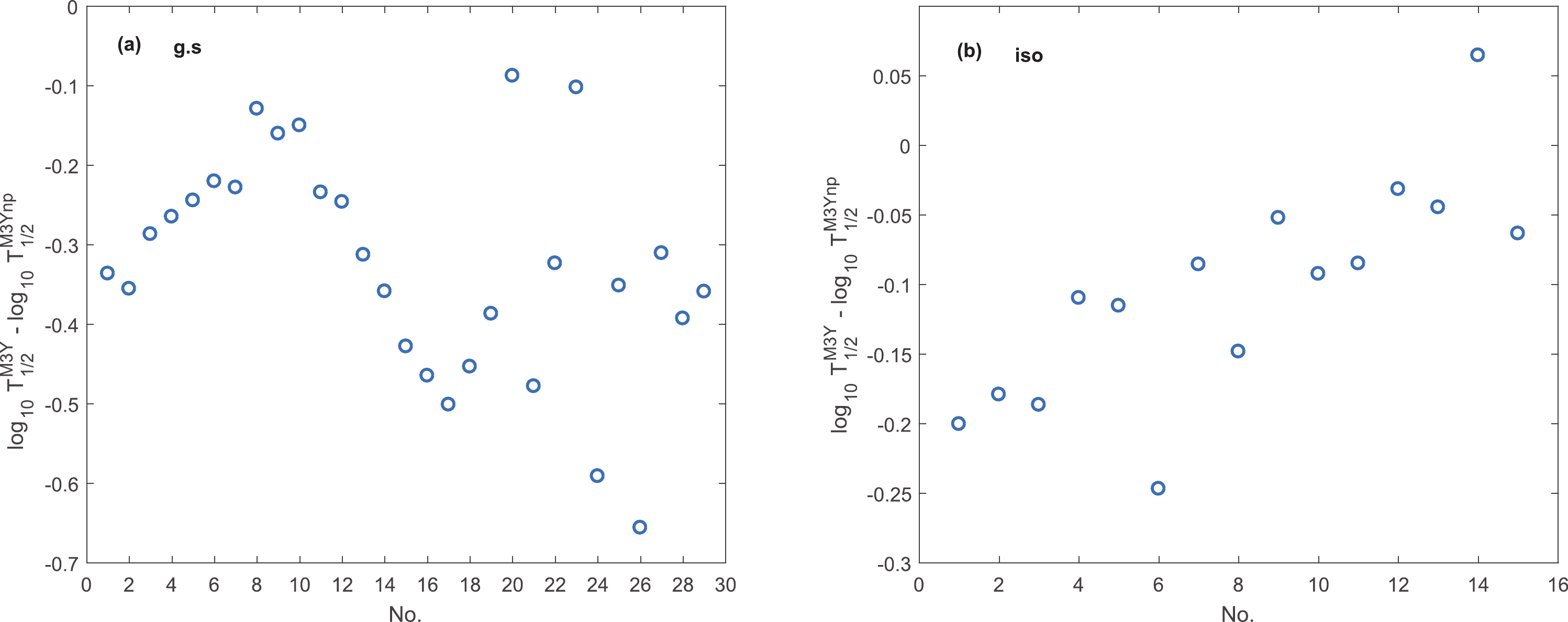Figure2. (color online) Difference between calculated half-lives with and without nuclear asymmetry parameter.

As already mentioned, spectroscopic factors for proton emission can be estimated by the non-occupation probability of the relevant level in the daughter nucleus. These values have been calculated in the RMF+BCS formalism. The computer code DIZ [35], extended for odd particle numbers in Ref. [36], has been employed. We have employed two standard parameters, NL1 [37] and NL3 [38], for RMF calculation. A constant pairing gap approach has been assumed, with the values of the pairing gap being estimated from the experimental odd-even mass difference, if available, or its corresponding estimate from semi-microscopic binding energy values. Obtained values for spectroscopic factors are presented in Table 1. Except in some cases for isomeric transition, NL1 and NL3 give similar results. Many of the daughter nuclei are found to be nearly spherical at low energy, and these have been indicated in the table.

No.	Parent	$ S_p({\rm NL1}) $	$ S_p({\rm NL3}) $	No.	Parent	$ S_p({\rm NL1}) $	$ S_p({\rm NL3}) $
1	$ ^{109} $I	0.838	0.789	1	$^{141{\rm m}}$Ho	0.505	0.658
2	$ ^{112} $Cs	0.584	0.753	2	$^{146{\rm m}}$Tm	0.923	0.905
3	$ ^{113} $Cs	0.571	0.741	3	$^{147{\rm m}}$Tm	0.331	0.508
4	$ ^{117} $La	0.743	0.744	4	$^{150{\rm m}}$Lu	0.702	0.817
5	$ ^{121} $Pr	0.911	0.907	5	$^{151{\rm m}}$Lu	0.622	0.737
6	$ ^{130} $Eu	0.697	0.852	6	$^{156{\rm m}}$Ta*	0.496	0.401
7	$ ^{131} $Eu	0.678	0.844	7	$^{159{\rm m}}$Re*	0.387	0.303
8	$ ^{135} $Tb	0.868	0.829	8	$^{161{\rm m}}$Re*	0.376	0.272
9	$ ^{140} $Ho	0.745	0.645	9	$^{165{\rm m}}$Ir*	0.245	0.163
10	$ ^{141} $Ho	0.747	0.650	10	$^{166{\rm m}}$Ir	0.771	0.620
11	$ ^{144} $Tm	0.558	0.418	11	$^{167{\rm m}}$Ir	0.789	0.641
12	$ ^{145} $Tm	0.918	0.898	12	$^{170{\rm m}}$Au*	0.137	0.086
13	$ ^{146} $Tm	0.923	0.905	13	$^{171{\rm m}}$Au*	0.43	0.087
14	$ ^{147} $Tm	0.685	0.596	14	$^{177{\rm m}}$Tl*	0.056	0.083
15	$ ^{150} $Lu	0.753	0.671	15	$^{185{\rm m}}$Bi*	0.986	0.985
16	$ ^{151} $Lu	0.737	0.648
17	$ ^{155} $Ta*	0.509	0.402
18	$ ^{156} $Ta*	0.459	0.651
19	$ ^{157} $Ta*	0.681	0.812
20	$ ^{159} $Re*	0.678	0.730
21	$ ^{160} $Re*	0.402	0.549
22	$ ^{161} $Re*	0.609	0.768
23	$ ^{164} $Ir*	0.339	0.475
24	$ ^{166} $Ir	0.576	0.713
25	$ ^{167} $Ir	0.745	0.845
26	$ ^{170} $Au*	0.339	0.339
27	$ ^{171} $Au*	0.531	0.660
28	$ ^{176} $Tl*	0.296	0.408
29	$ ^{177} $Tl*	0.291	0.414

Table1.Spectroscopic factor of proton emitters. Daughters of nuclei marked with '$ * $' are nearly spherical at low excitation energy.

Using assault frequency and tunneling probability as functions of the asymmetry parameter and calculated values of spectroscopic factor, the proton emission half-lives are obtained. The difference between calculated half-lives and experimental values for ground state and isomeric transitions can be observed in Fig. 3(a) and (b), respectively. The obtained half-lives are in good agreement with experiment.
Figure3. (color online) Difference between calculated half-lives and experimental data for (a) ground state and (b) isomeric transitions. M3Ynp (NL1) and M3Ynp (NL3) stand for calculated half-lives with asymmetry parameter and spectroscopic factor with the RMF+BCS model.

The adjustable parameters of the empirical formulas and corresponding rms errors are given in Tables 2 and 3. Table 2 presents the fitted parameters for the empirical formula for $ \log_{10} T_{1/2}^{\rm red} $, as given in Eq. (11). Four categories have been considered for evaluation of the nuclear deformation and asymmetry parameter. Categories (I) to (IV) correspond to the empirical formula $ \log_{10} T_{1/2}^{\rm red} $ without the deformation and asymmetry terms, with only the deformation term, with only the asymmetry term, and with both the deformation and asymmetry terms, respectively. For each category, we present the fitted parameters and corresponding rms values for the ground states, the isomeric states, and all transitions. Furthermore, for the ground state and all transitions, the corresponding data for odd-even and odd-odd proton emitters are given in the second vertical block of the table, separately. The first category, as the simplest form of $ \log_{10} T_{1/2}^{\rm red} $ with the minimum number of adjustable parameters, gives reasonable rms error values. For this case the rms error increases slightly for odd-even nuclei while a noticeable decrease, about 0.1, is obtained for odd-odd nuclei. In comparison with category I, lower values of rms errors are obtained for ground state, isomeric, and all transitions in category II. In this category the rms errors decrease for both odd-even and odd-odd divisions. The formula of category III gives lower values of rms error in comparison with category I. These results show that including the deformation or asymmetry terms can decrease the rms errors for different forms of transitions, odd-even and odd-odd ground state, isomeric, or all transitions. By considering both correction terms, the completed form of $ \log_{10} T_{1/2}^{\rm red} $ with lowest values of rms error are obtained in category IV. The calculated rms errors are lower than 0.3 for ground state (odd-even and odd-odd) and isomeric transitions.

Transition	Parameters	$ \sigma $	Parameters	$\sigma^{{\rm o-e/o-o}}$	Category
Ground	(0.432, ?2.138, ?13.701)	0.4578	(0.430, ?2.371, ?11.644)	0.4678
			(0.439, ?1.668, ?18.073)	0.3507
Isomeric	(0.384, ?0.664, ?23.242)	0.3505			(I)
			(0.409, ?1.955, ?13.698)	0.4997
All	(0.413, ?1.833, ?14.985)	0.4822	(0.422, ?1.485, ?18.578)	0.3943
Ground	(0.434, ?1.791,89.210, ?16.903)	0.3593	(0.428, ?1.910, 116.136, ?15.609)	0.2669
			(0.444, ?1.462, 52.092, ?20.184)	0.3152
Isomeric	(0.377, ?0.702, 77.508, ?22.606)	0.2999			(II)
			(0.407, ?1.5091, 115.878, ?16.877)	0.3330
All	(0.414, ?1.509, 94.610, ?18.013)	0.3899	(0.427, ?1.251, 57.189, ?20.987)	0.3667
Ground	(0.464, ?0.819, ?42.578, ?24.286)	0.4176	(0.481, ?0.210, ?70.55, ?28.747)	0.3458
			(0.498,1.132, ?80.948, ?40.760)	0.2944
Isomeric	(0.345, ?2.464, 39.942, ?8.140)	0.2870			(III)
			(0.405, ?2.197, 6.836, ?11.832)	0.4982
All	(0.409, ?2.031, 5.643, ?13.447)	0.4812	(0.484, 1.535, ?85.279, ?42.966)	0.3306
Ground	(0.433, ?1.816, 0.881,90.028, ?16.714)	0.3593	(0.425, ?1.987, 2.939, 119.431, ?15.009)	0.2668
			(0.489, 0.714, ?66.927, 17.012, ?37.520)	0.2919
Isomeric	(0.353, ?2.001,29.3195, 31.020, ?11.902)	0.2828			(IV)
			(0.399, ?2.044, 13.012, 118.035, ?13.383)	0.3249
All	(0.407, ?1.944, 12.666, 97.60, ?14.658)	0.3838	(0.479, 1.325, ?77.883, 12.827, ?41.385)	0.3295

Table2.Parameters for the empirical formula for $ \log_{10} T_{1/2}^{\rm red} $ in Eq. (11), for ground state (29 nuclei), isomeric (15 nuclei), and all transitions. The first to fourth sets of data, categories I to IV, correspond to the calculation without deformation and asymmetry, just with deformation, just with asymmetry, and with both deformation and asymmetry, respectively.

Transition	Parameters	$ \sigma $	Parameters	$\sigma^{\rm o-e/o-o}$	Category
Ground	(0.032, 0.825, ?0.151, ?26.545)	0.3505	(0.047, 0.819, ?0.540, ?26.219)	0.3091
			(0.022, 0.852, 0.202, ?27.686)	0.2564
Isomeric	(0.120, 0.337, ?2.404, ?14.061)	0.4220			(I)
			(0.032, 0.840, ?0.144, ?26.903)	0.4183
All	(0.023, 0.845, 0.109, ?27.176)	0.3976	(0.002, 0.935, 0.761, ?30.084)	0.2549
Ground	(0.014, 0.908, 0.374, ?29.085, 65.348)	0.2680	(0.024, 0.896, 0.091, ?28.630, 75.488)	0.1555
			(0.006, 0.937, 0.663, ?30.197, 35.209)	0.2321
Isomeric	(0.142, 0.211, ?2.782, ?11.848, 215.944)	0.2783			(II)
			(0.008, 0.935, 0.545, ?29.881, 88.050)	0.3142
All	(0.005, 0.933, 0.641, ?29.88, 73.00)	0.3286	(-0.010, 1.002, 1.107, ?32.069, 37.513)	0.2317
Ground	(0.011, 0.936, 0.446, ?29.073, ?10.909)	0.3161	(0.020, 0.949, ?29.116, ?14.129)	0.2386
			(0.014, 0.892, 0.415, ?28.659, ?2.604)	0.254
Isomeric	(0.235, ?0.221, ?5.431, ?1.379, 28.833)	0.2414			(III)
			(0.026, 0.869, 0.020, ?27.423, ?4.809)	0.4091
All	(0.019, 0.867, 0.221, ?27.596, ?3.029)	0.3945	(-0.004, 0.967, 0.927, ?30.859, ?2.448)	0.2530
Ground	(0.011, 0.924, 0.456, ?29.407, ?2.271, 60.099)	0.2667	(0.019, 0.923, 0.222, ?29.139, ?3.944, 66.096)	0.1492
			(0.009, 0.919, 0.564, ?29.790, 1.780, 38.753)	0.2312
Isomeric	(0.213, ?0.123, ?4.736, ?3.954, 20.271, 116.391)	0.1990			(IV)
			(0.009, 0.933, 0.534, ?29.856, 0.620, 89.305)	0.3140
All	(0.008, 0.916, 0.559, ?29.578, 37.856, 81.051)	0.3215	(-0.005, 0.974, 0.964, ?31.484, 3.142, 45.284)	0.2293

Table3.Same as Table 2, but for $ \log_{10} T_{1/2} $, Eq. (12).

The adjustable parameters of the empirical formula $ \log_{10} T $ in Eq. (12), and corresponding rms error, are presented in Table 3. The categories and divisions in this table are the same as in Table 2. Similar behaviors are observed in this table. That is, inclusion of deformation and asymmetry terms reduces the error, and combining both terms can decrease the rms error significantly.
Moreover, comparison between the two empirical formulas shows that, except for the isomeric transition formula in the first category, using Eq. (12) for $ \log_{10} T $, we obtain smaller rms error values for all formulas of categories and divisions. In most cases this reduction is about 0.1.
In order to evaluate the contribution of nuclear deformation and asymmetry parameter terms in the empirical formula for $ \log_{10} T $, the difference between experimental half-lives and corresponding values calculated by means of the parameters of categories I, II, and III, given in Table 3, are plotted in Fig. 4 (a)-(c). Figure 4 (a), (b), and (c) show the deviations for odd-even ground state, odd-odd ground state, and isomeric transitions, respectively. As can be seen, in most cases the difference decreases when the deformation term or asymmetry term is added. The role of the asymmetry term in reduction of the rms of isomeric transitions is apparent. Similar results, which are not presented here, are obtained for $ \log_{10} T_{1/2}^{\rm red} $.
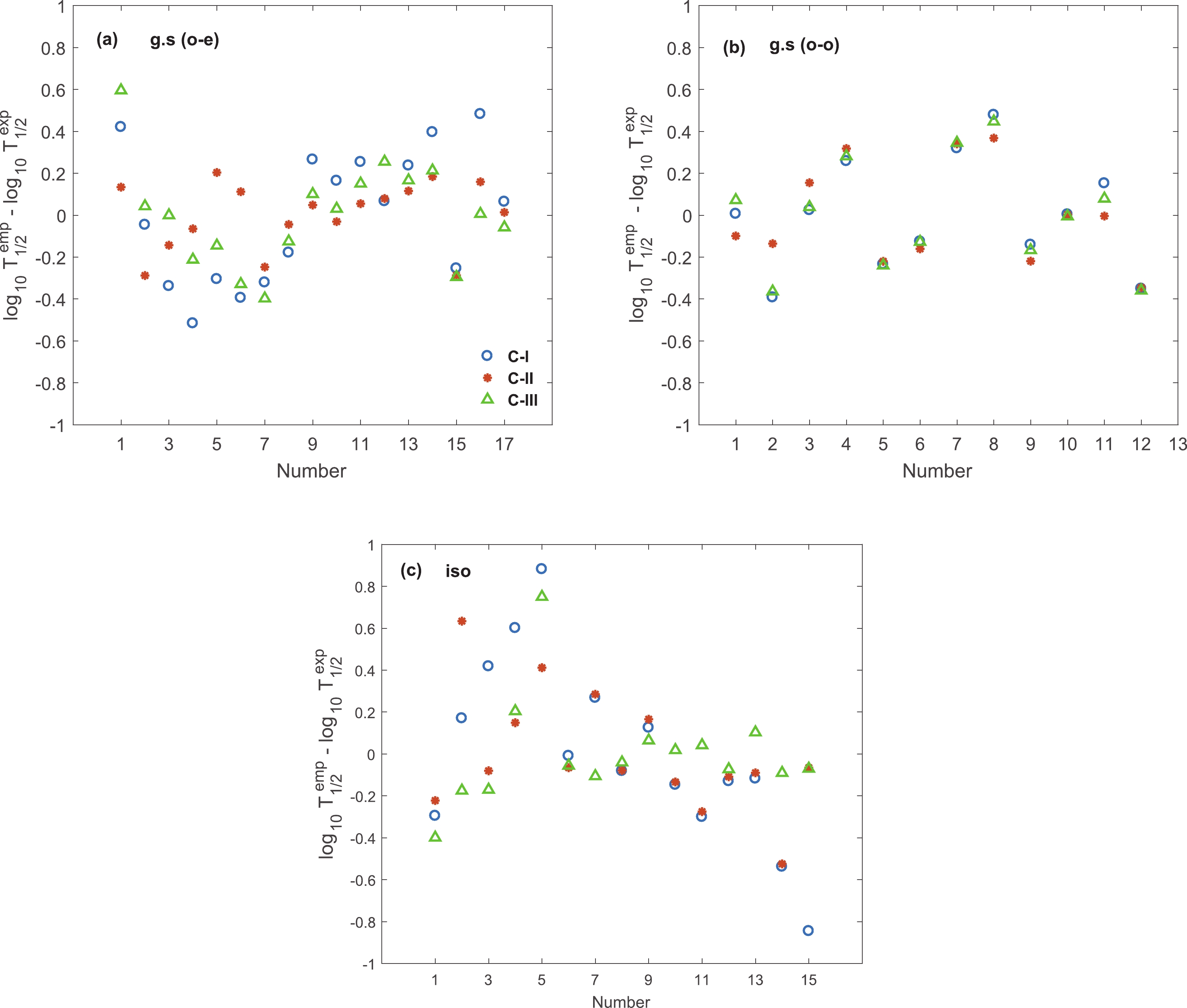Figure4. (color online) Difference between calculated and experimental half-lives with parameters of Table 3. The numbers in (a) and (b) correspond to the odd-even and odd-odd nuclei in Table 1.

Figure 5 (a)-(c) shows the difference between experimental data and calculated half-lives of ground state odd-even, odd-odd, and isomeric transitions with the lowest rms, category IV, for both the empirical formulas. These figures clearly show that inclusion of both deformation and asymmetry terms effectively reduces the deviation between empirical results and experiment, as well as indicating the crucial role of the deformation and asymmetry terms. Very good agreement between theory and experiment is observed, especially for the second form of empirical formula $ \log T $, which reveals the reliability of these modified formulas for prediction of the proton emission half-lives.
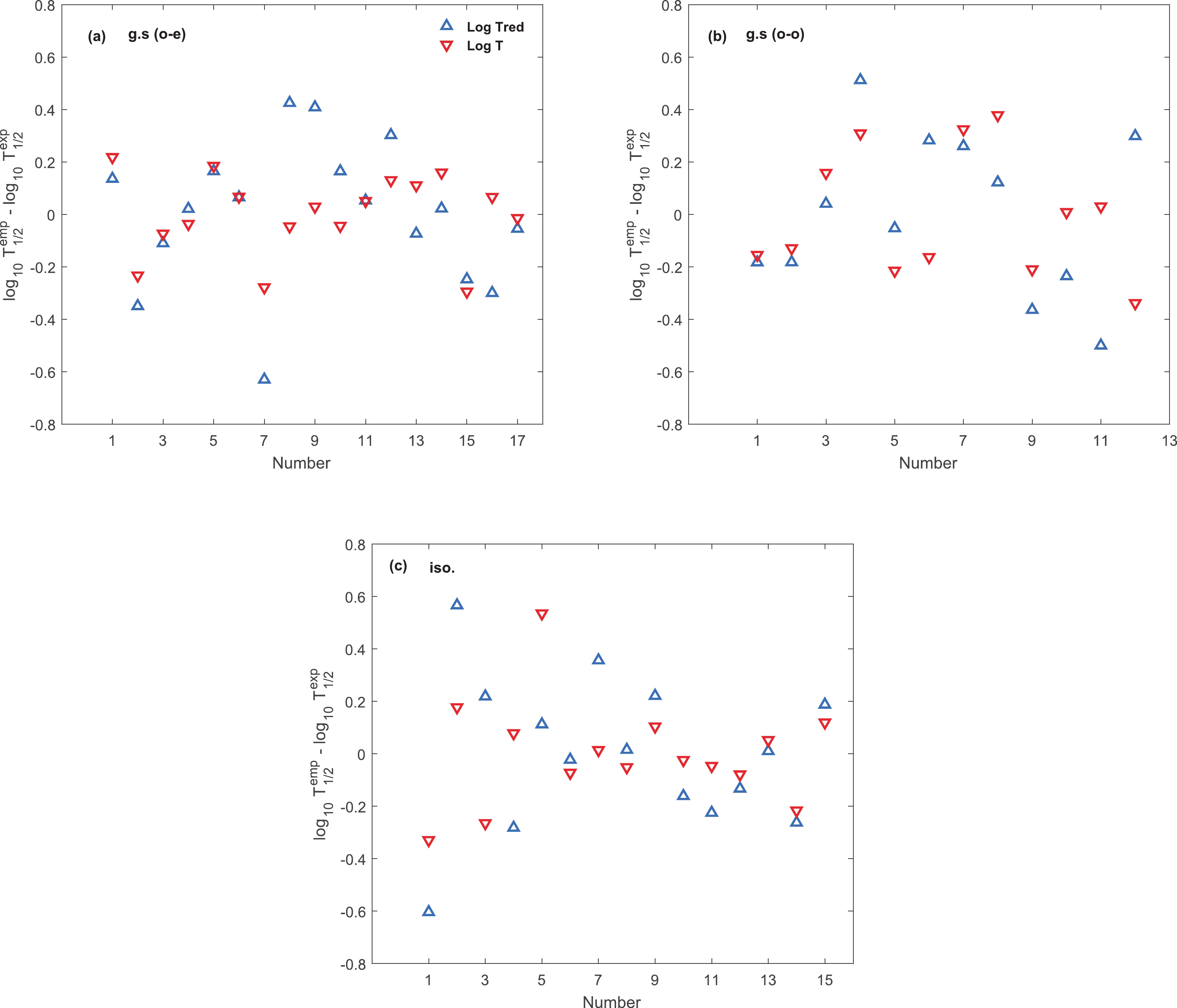Figure5. (color online) Difference between calculated and experimental half-lives for the formula with the lowest rms error, category IV.

In this paper, the effect of the nuclear asymmetry parameter on the calculated half lives and empirical formulas of 44 proton emitters have been investigated. The WKB method and single-folding nuclear potential with inclusion of the Bohr-Sommerfeld quantization condition have been employed for calculation of the tunneling probability and assault frequency. Spectroscopic factors have been calculated in the RMF formalism using two standard parameter sets, NL1 and NL3. Adding the Lane nuclear potential to the effective potential gives the total nuclear potential as an explicit function of the asymmetry parameter. Imposing a quantization condition causes this dependence to disappear. Therefore, by inclusion of the asymmetry parameter dependent radius and surface diffuseness in the nuclear density expression, the normalized nuclear potential through quantization condition, tunneling probability, assault frequency, and decay half-life are obtained as functions of the asymmetry parameter. Because of the neutron-deficient nature of the proton emitters, the asymmetry parameter is a relatively small quantity. However, since it directly affects the surface diffuseness, remarkable changes in the calculated half-lives, as obtained here, can be anticipated.
The remarkable contribution of the asymmetry parameter in theoretical calculations justifies the explicit presence of a correction term as a function of asymmetry parameter in empirical formulas. The dependence of two forms of empirical formulas on the asymmetry term have been investigated in different categories of transitions and specialized divisions of odd-even and odd-odd ground state and all transitions. The inclusion of this modification can reduce the rms errors in all cases, and for isomeric and odd-even and odd-odd ground state transitions the reduction is very apparent, especially for the second type of empirical formula, in which the rms error reaches about 0.2 (corresponding to a 43% relative reduction). The data has been fitted for the quadrupole deformation term separately and, as expected, very good results have been obtained. Therefore, the presence of both deformation and asymmetry terms in empirical formulas have been evaluated and the lowest rms error values have been achieved for both formulas. The rms error has been brought down to less than 0.2 for the isomeric and ground state odd-even transitions, and better agreement between theory and experiment is observed for the second type of formula, with explicit dependence on angular momentum, deformation, and asymmetry parameter.