


HTML
--> --> -->The charged charmonium-like state
$ {\cal{R}}_{Z_c} \equiv {{\cal{B}}(Z_c(3900) \rightarrow \eta_c\rho) \over {\cal{B}}(Z_c(3900) \rightarrow J/\psi\pi)} \, , $  | (1) |
| interpretations |   | methods/models |
| compact tetraquark |   | Type-I diquark-antidiquark model [40] |
  | Type-II diquark-antidiquark model [40] | |
  | QCD sum rules [30] | |
  | QCD sum rules [31] | |
  | QCD sum rules [32] | |
  | covariant quark model [33] | |
| hadronic molecule |   | Non-Relativistic effective field theory [40] |
  | light front model [34] | |
  | effective field theory [35] | |
  | covariant quark model [33] |
Table1.The relative branching ratio
In this paper we study the decay properties of the
$ [cq][\bar c \bar q]\, , \; \; [\bar c q][\bar q c]\, , \; \; {\rm{and}} \; \; [\bar c c][\bar q q] \, . $  |
There are eight independent
$ \eta^{{\cal{Z}}}_{\mu} = \epsilon^{abe} \epsilon^{cde}\; q_a^T{\mathbb{C}}\gamma_{\mu} c_b \; \bar q_c \gamma_5{\mathbb{C}}\bar c_d^T - \{ \gamma_{\mu} \leftrightarrow \gamma_5 \} \, , $  | (2) |
The above current is useful from the viewpoints of both effective field theory and QCD sum rules. Note that there are various quark-based effective field theories, which have been successfully applied to describe the meson and baryon systems, such as the Non-Relativistic QCD for the heavy quarkonium system [56, 57]:
$ \begin{split} {\cal{L}}_{\rm{NRQCD}} =& \psi^{\dagger} \left\{ {\rm i} D_0 + \cdots \right\} \psi + \chi^{\dagger} \left\{ {\rm i} D_0 + \cdots \right\} \chi \\&+ {f_1(^1S_0) \over m_1 m_2} \psi^{\dagger} \chi \chi^{\dagger} \psi + {f_1(^3S_0) \over m_1 m_2} \psi^{\dagger} {{\sigma}} \chi \chi^{\dagger} {{\sigma}} \psi \\ &+ {f_8(^1S_0) \over m_1 m_2} \psi^{\dagger} T^a\chi \chi^{\dagger} T^a \psi \\ &+ {f_8(^3S_0) \over m_1 m_2} \psi^{\dagger} T^a {{\sigma}} \chi \chi^{\dagger} T^a {{\sigma}} \psi + \cdots \, . \end{split} $  | (3) |
Compared with this, the quark-based effective field theory for the multiquark system is much more difficult [24]. Let us attempt to do this for the
$ \begin{split} {\cal{L}} = & c_0 \times \eta^{{\cal{Z}}}_{\mu} \times \left(\eta^{{{\cal{Z}}},\mu}\right)^{\dagger} \\ = &c_0 \times \left( \epsilon^{abe} \epsilon^{cde}\; q_a^T{\mathbb{C}}\gamma_{\mu} c_b \; \bar q_c \gamma_5{\mathbb{C}}\bar c_d^T - \{ \gamma_{\mu} \leftrightarrow \gamma_5 \} \right) \\& \times \left( \epsilon^{a^{\prime} b^{\prime} e^{\prime} } \epsilon^{c^{\prime} d^{\prime} e^{\prime} }\; \bar c_{b^{\prime}} \gamma^\mu {\mathbb{C}} \bar q_{a^{\prime}}^T \; c_{d^{\prime}}^T {\mathbb{C}} \gamma_5 q_{c^{\prime}} - \{ \gamma_{\mu} \leftrightarrow \gamma_5 \} \right) \, , \end{split} $  | (4) |
$ \begin{split} {\cal{L}} =& c_0 \times \Big( + {1\over3} \; \bar c_{a} \gamma_5 c_a \; \bar q_{b} \gamma_{\mu} q_b - {1\over3} \; \bar c_{a} \gamma_{\mu} c_a \; \bar q_{b} \gamma_5 q_b \\ & + {{\rm i}\over3} \; \bar c_{a} \gamma^\nu \gamma_5 c_a \; \bar q_{b} \sigma_{\mu\nu} q_b - {{\rm i}\over3} \; \bar c_{a} \sigma_{\mu\nu} c_a \; \bar q_{b} \gamma^\nu \gamma_5 q_b \\ & - {1\over4} \; {\lambda^n_{ab}}{\lambda^n_{cd}} \; \bar c_{a} \gamma_5 c_b \; \bar q_{c} \gamma_{\mu} q_d \\ & + {1\over4} \; {\lambda^n_{ab}}{\lambda^n_{cd}} \; \bar c_{a} \gamma_{\mu} c_b \; \bar q_{c} \gamma_5 q_d \\ & - {{\rm i}\over4} \; {\lambda^n_{ab}}{\lambda^n_{cd}} \; \bar c_{a} \gamma^\nu \gamma_5 c_b \; \bar q_{c} \sigma_{\mu\nu} q_d \\ & + {{\rm i}\over4} \; {\lambda^n_{ab}}{\lambda^n_{cd}} \; \bar c_{a} \sigma_{\mu\nu} c_b \; \bar q_{c} \gamma^\nu \gamma_5 q_d \Big) \\ & \times \left( \epsilon^{a^{\prime} b^{\prime} e^{\prime} } \epsilon^{c^{\prime} d^{\prime} e^{\prime} }\; \bar c_{b^{\prime}} \gamma^\mu {\mathbb{C}} \bar q_{a^{\prime}}^T \; c_{d^{\prime}}^T {\mathbb{C}} \gamma_5 q_{c^{\prime}} - \{ \gamma_{\mu} \leftrightarrow \gamma_5 \} \right) \, . \end{split} $  | (5) |
Considering that the meson operators,
| operators |   | mesons |   | couplings | decay constants |
  |   | – |   | – | – |
  |   |   |   |   |   |
  |   |   |   |   |   |
  |   |   |   |   |   |
  |   |   |   | ||
  |   |   |   |   |   |
  |   |   |   | ||
  |   |   |   |   |   |
  |   |   |   |   |   |
  |   |   |   |   |   |
  |   |   |   |   |   |
  |   |   |   | ||
  |   |   |   |   |   |
  |   |   |   | ||
  |   |   |   |   |   |
  |   |   |   |   |   |
  |   |   |   |   |   |
  |   |   |   |   |   |
  |   |   |   | ||
  |   |   |   |   |   |
| – |   | – | – |
Table2.Couplings of meson operators to meson states. Color indices are omitted for simplicity.
The current
$ \langle 0 | \eta^{{\cal{Z}}}_{\mu} | Z_c \rangle = f_{Z_c} \epsilon_{\mu} \, . $  | (6) |
$ \begin{split} & \langle 0 | \eta^{{\cal{Z}}}_{\mu} | \eta_c \rho \rangle = {1\over3} \langle 0 | \bar c_{a} \gamma_5 c_a | \eta_c \rangle \langle 0 | \bar q_{b} \gamma_{\mu} q_b | \rho \rangle + \cdots \, , \\ & \langle 0 | \eta^{{\cal{Z}}}_{\mu} | J/\psi \pi \rangle = - {1\over3} \langle 0 | \bar c_{a} \gamma_{\mu} c_a | J/\psi \rangle \langle 0 | \bar q_{b} \gamma_5 q_b | \pi \rangle + \cdots \, . \end{split} $  | (7) |
In the above equations, we have worked within the naive factorization scheme, so our uncertainty is significantly larger than the well-developed QCD factorization method [62-64], which has been widely and successfully applied to study weak and radiative decay properties of conventional (heavy) hadrons, e.g., see Refs. [65, 66]. However, given that we still do not fully understand the internal structure of the
In this study, we shall examine the strong decay properties of the
This paper is organized as follows. In Sec. 2 we systematically construct all the tetraquark currents of
 Figure1. (color online) Three types of tetraquark currents. Quarks are shown in red/green/blue color, and antiquarks are shown in cyan/magenta/yellow color.
 $ \begin{split}& \eta(x,y) = [q^T_a(x)\; {\mathbb{C}} \Gamma_1\; c_b(x)] \times [\bar q_c(y)\; \Gamma_2 {\mathbb{C}}\; \bar c_d^T(y)] \, , \\ & \xi(x,y) = [\bar c_a(x)\; \Gamma_3\; q_b(x)] \times [\bar q_c(y)\; \Gamma_4\; c_d(y)] \, , \\ & \theta(x,y) = [\bar c_a(x)\; \Gamma_5\; c_b(x)] \times [\bar q_c(y)\; \Gamma_6\; q_d(y)] \, , \end{split} $  | (8) |
2
2.1.$ [qc][\bar q \bar c] $![]()
![]()
currents $ \eta_{\mu}^i(x,y) $![]()
![]()
There are altogether eight independent $ \begin{split} & \eta^1_{\mu} = q_a^T{\mathbb{C}}\gamma_{\mu} c_b \; \bar q_{a} \gamma_5{\mathbb{C}}\bar c_{b}^T - q_a^T{\mathbb{C}}\gamma_5 c_b \; \bar q_{a} \gamma_{\mu}{\mathbb{C}}\bar c_{b}^T \, , \\ & \eta^2_{\mu} = q_a^T{\mathbb{C}}\gamma_{\mu} c_b \; \bar q_{b} \gamma_5{\mathbb{C}}\bar c_{a}^T - q_a^T{\mathbb{C}}\gamma_5 c_b \; \bar q_{b} \gamma_{\mu}{\mathbb{C}}\bar c_{a}^T \, , \\ & \eta^3_{\mu} = q_a^T{\mathbb{C}}\gamma^\nu c_b \; \bar q_{a} \sigma_{\mu\nu} \gamma_5{\mathbb{C}}\bar c_{b}^T - q_a^T{\mathbb{C}}\sigma_{\mu\nu} \gamma_5 c_b \; \bar q_{a} \gamma^\nu{\mathbb{C}}\bar c_{b}^T \, , \\ & \eta^4_{\mu} = q_a^T{\mathbb{C}}\gamma^\nu c_b \; \bar q_{b} \sigma_{\mu\nu} \gamma_5{\mathbb{C}}\bar c_{a}^T - q_a^T{\mathbb{C}}\sigma_{\mu\nu} \gamma_5 c_b \; \bar q_{b} \gamma^\nu{\mathbb{C}}\bar c_{a}^T \, , \\ & \eta^5_{\mu} = q_a^T{\mathbb{C}}\gamma_{\mu} \gamma_5 c_b \; \bar q_{a}{\mathbb{C}}\bar c_{b}^T - q_a^T{\mathbb{C}}c_b \; \bar q_{a} \gamma_{\mu} \gamma_5{\mathbb{C}}\bar c_{b}^T \, , \\ & \eta^6_{\mu} = q_a^T{\mathbb{C}}\gamma_{\mu} \gamma_5 c_b \; \bar q_{b}{\mathbb{C}}\bar c_{a}^T - q_a^T{\mathbb{C}}c_b \; \bar q_{b} \gamma_{\mu} \gamma_5{\mathbb{C}}\bar c_{a}^T \, , \\ & \eta^7_{\mu} = q_a^T{\mathbb{C}}\gamma^\nu \gamma_5 c_b \; \bar q_{a} \sigma_{\mu\nu}{\mathbb{C}}\bar c_{b}^T - q_a^T{\mathbb{C}}\sigma_{\mu\nu} c_b \; \bar q_{a} \gamma^\nu \gamma_5{\mathbb{C}}\bar c_{b}^T \, , \\ & \eta^8_{\mu} = q_a^T{\mathbb{C}}\gamma^\nu \gamma_5 c_b \; \bar q_{b} \sigma_{\mu\nu}{\mathbb{C}}\bar c_{a}^T - q_a^T{\mathbb{C}}\sigma_{\mu\nu} c_b \; \bar q_{b} \gamma^\nu \gamma_5{\mathbb{C}}\bar c_{a}^T \, . \end{split} $  | (9) |
In the "type-II" diquark-antidiquark model proposed in Ref. [6], the ground-state tetraquarks can be written in the spin basis as
$ |0_{qc}1_{\bar q \bar c}; 1^{+-} \rangle = {1\over\sqrt2} \left(| 0_{qc}, 1_{\bar q \bar c} \rangle_{J = 1} - |1_{qc}, 0_{\bar q \bar c} \rangle_{J = 1} \right) \, . $  | (10) |
$ \begin{split} \eta^{{\cal{Z}}}_{\mu}(x,y) & = \eta^1_{\mu}([uc][\bar d \bar c]) - \eta^2_{\mu}([uc][\bar d \bar c]) \\ & = u_a^T(x){\mathbb{C}}\gamma_{\mu} c_b(x) \\&\times\left( \bar d_{a}(y) \gamma_5{\mathbb{C}}\bar c_{b}^T(y) - \{ a \leftrightarrow b \} \right) \\& - \; \{ \gamma_{\mu} \leftrightarrow \gamma_5 \} \, . \end{split} $  | (11) |
2
2.2.$ [\bar c q][\bar q c] $![]()
![]()
currents $ \xi_{\mu}^i(x,y) $![]()
![]()
There are altogether eight independent $ \begin{split} & \xi^1_{\mu} = \bar c_{a} \gamma_{\mu} q_a \; \bar q_{b} \gamma_5 c_b + \bar c_{a} \gamma_5 q_a \; \bar q_{b} \gamma_{\mu} c_b \, , \\& \xi^2_{\mu} = \bar c_{a} \gamma^\nu q_a \; \bar q_{b} \sigma_{\mu\nu} \gamma_5 c_b - \bar c_{a} \sigma_{\mu\nu} \gamma_5 q_a \; \bar q_{b} \gamma^\nu c_b \, , \\ & \xi^3_{\mu} = \bar c_{a} \gamma_{\mu} \gamma_5 q_a \; \bar q_{b} c_b - \bar c_{a} q_a \; \bar q_{b} \gamma_{\mu} \gamma_5 c_b \, , \\& \xi^4_{\mu} = \bar c_{a} \gamma^\nu \gamma_5 q_a \; \bar q_{b} \sigma_{\mu\nu} c_b + \bar c_{a} \sigma_{\mu\nu} q_a \; \bar q_{b} \gamma^\nu \gamma_5 c_b \, , \\& \xi^5_{\mu} = {\lambda^n_{ab}}{\lambda^n_{cd}} \; \left( \bar c_{a} \gamma_{\mu} q_b \; \bar q_{c} \gamma_5 c_d + \bar c_{a} \gamma_5 q_b \; \bar q_{c} \gamma_{\mu} c_d \right) \, , \end{split} $  |
$ \begin{split} & \xi^6_{\mu} = {\lambda^n_{ab}}{\lambda^n_{cd}} \; \left( \bar c_{a} \gamma^\nu q_b \; \bar q_{c} \sigma_{\mu\nu} \gamma_5 c_d - \bar c_{a} \sigma_{\mu\nu} \gamma_5 q_b \; \bar q_{c} \gamma^\nu c_d \right) \, , \\ & \xi^7_{\mu} = {\lambda^n_{ab}}{\lambda^n_{cd}} \; \left( \bar c_{a} \gamma_{\mu} \gamma_5 q_b \; \bar q_{c} c_d - \bar c_{a} q_b \; \bar q_{c} \gamma_{\mu} \gamma_5 c_d \right) \, , \\& \xi^8_{\mu} = {\lambda^n_{ab}}{\lambda^n_{cd}} \; \left( \bar c_{a} \gamma^\nu \gamma_5 q_b \; \bar q_{c} \sigma_{\mu\nu} c_d + \bar c_{a} \sigma_{\mu\nu} q_b \; \bar q_{c} \gamma^\nu \gamma_5 c_d \right) \, . \end{split} $  | (12) |
$ | D \bar D^*; 1^{+-} \rangle = {1\over\sqrt2} \left(| D \bar D^* \rangle_{J = 1} - | \bar D D^* \rangle_{J = 1} \right) \, , $  | (13) |
$ \begin{split} \xi^{{\cal{Z}}}_{\mu}(x,y) & = \xi^1_{\mu}([\bar c u][\bar d c]) \\& = \bar c_{a}(x) \gamma_{\mu} u_a(x) \; \bar d_{b}(y) \gamma_5 c_b(y) + \{ \gamma_{\mu} \leftrightarrow \gamma_5 \} \, . \end{split} $  | (14) |
2
2.3.$ [\bar c c][\bar q q] $![]()
![]()
currents $ \theta_{\mu}^i(x,y) $![]()
![]()
There are altogether eight independent $ \begin{split} & \theta^1_{\mu}(x,y) = \bar c_{a}(x) \gamma_5 c_a(x) \; \bar q_{b}(y) \gamma_{\mu} q_b(y) \, , \\ & \theta^2_{\mu}(x,y) = \bar c_{a}(x) \gamma_{\mu} c_a(x) \; \bar q_{b}(y) \gamma_5 q_b(y) \, , \\ & \theta^3_{\mu}(x,y) = \bar c_{a}(x) \gamma^\nu \gamma_5 c_a(x) \; \bar q_{b}(y) \sigma_{\mu\nu} q_b(y) \, , \\ & \theta^4_{\mu}(x,y) = \bar c_{a}(x) \sigma_{\mu\nu} c_a(x) \; \bar q_{b}(y) \gamma^\nu \gamma_5 q_b(y) \, , \\ & \theta^5_{\mu}(x,y) = {\lambda^n_{ab}}{\lambda^n_{cd}} \; \bar c_{a}(x) \gamma_5 c_b(x) \; \bar q_{c}(y) \gamma_{\mu} q_d(y) \, , \\& \theta^6_{\mu}(x,y) = {\lambda^n_{ab}}{\lambda^n_{cd}} \; \bar c_{a}(x) \gamma_{\mu} c_b(x) \; \bar q_{c}(y) \gamma_5 q_d(y) \, , \\ & \theta^7_{\mu}(x,y) = {\lambda^n_{ab}}{\lambda^n_{cd}} \; \bar c_{a}(x) \gamma^\nu \gamma_5 c_b(x) \; \bar q_{c}(y) \sigma_{\mu\nu} q_d(y) \, , \\ & \theta^8_{\mu}(x,y) = {\lambda^n_{ab}}{\lambda^n_{cd}} \; \bar c_{a}(x) \sigma_{\mu\nu} c_b(x) \; \bar q_{c}(y) \gamma^\nu \gamma_5 q_d(y) \, . \end{split} $  | (15) |
Fierz rearrangement
We have applied the Fierz rearrangement of the Dirac and color indices to systematically study light baryon and tetraquark operators/currents in Refs. [41-54]. It can also be used to relate the above three types of tetraquark currents. To do this, we must use a) the Fierz transformation [74] in the Lorentz space to rearrange the Dirac indices, and b) the color rearrangement in the color space to rearrange the color indices. All the necessary equations can be found in Sec. 3.3.2 of Ref. [75].
In Eq. (5) the Fierz rearrangement is applied to local operators/currents. However, the Fierz rearrangement is actually a matrix identity, which is valid if the same quark field in the initial and final operators is at the same location. As an example, we can apply the Fierz rearrangement to transform the non-local current with the quark fields
Altogether, we obtain the following relation between the currents
$ \left( {\begin{array}{*{20}{c}}{\eta _\mu ^1}\\{\eta _\mu ^2}\\{\eta _\mu ^3}\\{\eta _\mu ^4}\\{\eta _\mu ^5}\\{\eta _\mu ^6}\\{\eta _\mu ^7}\\{\eta _\mu ^8}\end{array}} \right) = \left( {\begin{array}{*{20}{c}}{1/2}&{ - 1/2}&{i/2}&{ - i/2}&0&0&0&0\\{1/6}&{ - 1/6}&{i/6}&{ - i/6}&{1/4}&{ - 1/4}&{i/4}&{ - i/4}\\{3i/2}&{3i/2}&{ - 1/2}&{ - 1/2}&0&0&0&0\\{i/2}&{i/2}&{ - 1/6}&{ - 1/6}&{3i/4}&{3i/4}&{ - 1/4}&{ - 1/4}\\{1/2}&{1/2}&{ - i/2}&{ - i/2}&0&0&0&0\\{1/6}&{1/6}&{ - i/6}&{ - i/6}&{1/4}&{1/4}&{ - i/4}&{ - i/4}\\{3i/2}&{ - 3i/2}&{1/2}&{ - 1/2}&0&0&0&0\\{i/2}&{ - i/2}&{1/6}&{ - 1/6}&{3i/4}&{ - 3i/4}&{1/4}&{ - 1/4}\end{array}} \right) \times \left( {\begin{array}{*{20}{c}}{\theta _\mu ^1}\\{\theta _\mu ^2}\\{\theta _\mu ^3}\\{\theta _\mu ^4}\\{\theta _\mu ^5}\\{\theta _\mu ^6}\\{\theta _\mu ^7}\\{\theta _\mu ^8}\end{array}} \right){\mkern 1mu} , $  | (16) |
$ \left( {\begin{array}{*{20}{c}}{\eta _\mu ^1}\\{\eta _\mu ^2}\\{\eta _\mu ^3}\\{\eta _\mu ^4}\\{\eta _\mu ^5}\\{\eta _\mu ^6}\\{\eta _\mu ^7}\\{\eta _\mu ^8}\end{array}} \right) = \left( {\begin{array}{*{20}{c}}0&{i/6}&{ - 1/6}&0&0&{i/4}&{ - 1/4}&0\\0&{i/2}&{ - 1/2}&0&0&0&0&0\\{ - i/2}&0&0&{1/6}&{ - 3i/4}&0&0&{1/4}\\{ - 3i/2}&0&0&{1/2}&0&0&0&0\\{1/6}&0&0&{ - i/6}&{1/4}&0&0&{ - i/4}\\{1/2}&0&0&{ - i/2}&0&0&0&0\\0&{ - 1/6}&{i/2}&0&0&{ - 1/4}&{3i/4}&0\\0&{ - 1/2}&{3i/2}&0&0&0&0&0\end{array}} \right) \times \left( {\begin{array}{*{20}{c}}{\xi _\mu ^1}\\{\xi _\mu ^2}\\{\xi _\mu ^3}\\{\xi _\mu ^4}\\{\xi _\mu ^5}\\{\xi _\mu ^6}\\{\xi _\mu ^7}\\{\xi _\mu ^8}\end{array}} \right){\mkern 1mu} , $  | (17) |
$ \left( {\begin{array}{*{20}{c}}{\eta _\mu ^1}\\{\eta _\mu ^2}\\{\eta _\mu ^3}\\{\eta _\mu ^4}\\{\eta _\mu ^5}\\{\eta _\mu ^6}\\{\eta _\mu ^7}\\{\eta _\mu ^8}\end{array}} \right) = \left( {\begin{array}{*{20}{c}}0&0&0&0&{1/2}&{ - 1/2}&{i/2}&{ - i/2}\\0&{i/2}&{ - 1/2}&0&0&0&0&0\\0&0&0&0&{3i/2}&{3i/2}&{ - 1/2}&{ - 1/2}\\{ - 3i/2}&0&0&{1/2}&0&0&0&0\\0&0&0&0&{1/2}&{1/2}&{ - i/2}&{ - i/2}\\{1/2}&0&0&{ - i/2}&0&0&0&0\\0&0&0&0&{3i/2}&{ - 3i/2}&{1/2}&{ - 1/2}\\0&{ - 1/2}&{3i/2}&0&0&0&0&0\end{array}} \right) \times \left( {\begin{array}{*{20}{c}}{\xi _\mu ^1}\\{\xi _\mu ^2}\\{\xi _\mu ^3}\\{\xi _\mu ^4}\\{\theta _\mu ^1}\\{\theta _\mu ^2}\\{\theta _\mu ^3}\\{\theta _\mu ^4}\end{array}} \right){\mkern 1mu} , $  | (18) |
$ \left( {\begin{array}{*{20}{c}}{\xi _\mu ^1}\\{\xi _\mu ^2}\\{\xi _\mu ^3}\\{\xi _\mu ^4}\\{\xi _\mu ^5}\\{\xi _\mu ^6}\\{\xi _\mu ^7}\\{\xi _\mu ^8}\end{array}} \right) = \left( {\begin{array}{*{20}{c}}{ - 1/6}&{ - 1/6}&{ - i/6}&{ - i/6}&{ - 1/4}&{ - 1/4}&{ - i/4}&{ - i/4}\\{ - i/2}&{i/2}&{1/6}&{ - 1/6}&{ - 3i/4}&{3i/4}&{1/4}&{ - 1/4}\\{1/6}&{ - 1/6}&{ - i/6}&{i/6}&{1/4}&{ - 1/4}&{ - i/4}&{i/4}\\{i/2}&{i/2}&{1/6}&{1/6}&{3i/4}&{3i/4}&{1/4}&{1/4}\\{ - 8/9}&{ - 8/9}&{ - 8i/9}&{ - 8i/9}&{1/6}&{1/6}&{i/6}&{i/6}\\{ - 8i/3}&{8i/3}&{8/9}&{ - 8/9}&{i/2}&{ - i/2}&{ - 1/6}&{1/6}\\{8/9}&{ - 8/9}&{ - 8i/9}&{8i/9}&{ - 1/6}&{1/6}&{i/6}&{ - i/6}\\{8i/3}&{8i/3}&{8/9}&{8/9}&{ - i/2}&{ - i/2}&{ - 1/6}&{ - 1/6}\end{array}} \right) \times \left( {\begin{array}{*{20}{c}}{\theta _\mu ^1}\\{\theta _\mu ^2}\\{\theta _\mu ^3}\\{\theta _\mu ^4}\\{\theta _\mu ^5}\\{\theta _\mu ^6}\\{\theta _\mu ^7}\\{\theta _\mu ^8}\end{array}} \right){\mkern 1mu} . $  | (19) |
$ \sigma_{\mu\nu} \gamma_5 = {{\rm i}\over2} \epsilon_{\mu\nu\rho\sigma} \sigma^{\rho\sigma} \, . $  | (20) |
In this study, we require the following couplings, as summarized in Table 2:
1. The scalar operators
$ \langle 0 | \bar c_a c_a | \chi_{c0}(p) \rangle = m_{\chi_{c0}} f_{\chi_{c0}} \, , $  | (21) |
$ f_{\chi_{c0}} = 343\; {\rm{MeV}} \, . $  | (22) |
2. The pseudoscalar operators
$ \begin{split} & \langle 0 | \bar d_a {\rm i}\gamma_5 u_a | \pi^+(p) \rangle = \lambda_{\pi} = {f_{\pi^+} m_{\pi^+}^2 \over m_u + m_d} \, , \\ & \;\;\;\;\langle 0 | \bar c_a {\rm i}\gamma_5 c_a | \eta_c(p) \rangle = \lambda_{\eta_c} = {f_{\eta_c} m_{\eta_c}^2 \over 2 m_c} \, . \end{split} $  | (23) |
$ \begin{split} & \langle 0 | \bar d_a \gamma_{\mu} u_a | \rho^+(p, \epsilon) \rangle = m_{\rho} f_{\rho^+} \epsilon_{\mu} \, , \\ & \langle 0 | \bar c_a \gamma_{\mu} c_a | J/\psi(p, \epsilon) \rangle = m_{J/\psi} f_{J/\psi} \epsilon_{\mu} \, , \end{split} $  | (24) |
$ \begin{array}{l} \;\;\;f_{\rho^+} = 208\; {\rm{MeV}} \, , \;\;\; f_{J/\psi} = 418\; {\rm{MeV}} \, . \end{array} $  | (25) |
4. The axialvector operators
$ \langle 0 | \bar d_a \gamma_{\mu} \gamma_5 u_a | \pi^+(p) \rangle = {\rm i} p_{\mu} f_{\pi^+} \, , $  | (26) |
$ \langle 0 | \bar d_a \gamma_{\mu} \gamma_5 u_a | a_1(p, \epsilon) \rangle = m_{a_1} f_{a_1} \epsilon_{\mu} \, , $  | (27) |
$ \begin{array}{l} f_{\pi^+} = 130.2\; {\rm{MeV}} \, , \;\;\; f_{a_1} = 254\; {\rm{MeV}} \, . \end{array} $  | (28) |
$ \begin{split} & \langle 0 | \bar c_a \gamma_{\mu} \gamma_5 c_a | \eta_c(p) \rangle = {\rm i} p_{\mu} f_{\eta_c} \, , \\ & \langle 0 | \bar c_a \gamma_{\mu} \gamma_5 c_a | \chi_{c1}(p, \epsilon) \rangle = m_{\chi_{c1}} f_{\chi_{c1}} \epsilon_{\mu} \, , \end{split} $  | (29) |
$ \begin{array}{l} f_{\eta_c} = 387\; {\rm{MeV}} \, , \;\;\; f_{\chi_{c1}} = 335\; {\rm{MeV}} \, . \end{array} $  | (30) |
5. The tensor operators
$ \begin{split} & \langle 0 | \bar d_a \sigma_{\mu\nu} u_a | \rho^+(p, \epsilon) \rangle = {\rm i} f^T_{\rho} (p_{\mu}\epsilon_\nu - p_\nu\epsilon_{\mu}) \, , \\& \langle 0 | \bar d_a \sigma_{\mu\nu} u_a | b_1(p, \epsilon) \rangle = {\rm i} f^T_{b_1} \epsilon_{\mu\nu\alpha\beta} \epsilon^\alpha p^\beta \, , \end{split} $  | (31) |
$ \begin{array}{l} f_{\rho}^T = 159\; {\rm{MeV}} \, , \;\;\; f_{b_1}^T = 180\; {\rm{MeV}} \, . \end{array} $  | (32) |
$ \begin{split}& \langle 0 | \bar c_a \sigma_{\mu\nu} c_a | J/\psi(p, \epsilon) \rangle = {\rm i} f^T_{J/\psi} (p_{\mu}\epsilon_\nu - p_\nu\epsilon_{\mu}) \, , \\ & \langle 0 | \bar c_a \sigma_{\mu\nu} c_a | h_c(p, \epsilon) \rangle = {\rm i} f^T_{h_c} \epsilon_{\mu\nu\alpha\beta} \epsilon^\alpha p^\beta \, , \end{split} $  | (33) |
$ \begin{array}{l} f_{J/\psi}^T = 410\; {\rm{MeV}} \, , \;\;\; f_{h_c}^T = 235\; {\rm{MeV}} \, . \end{array} $  | (34) |
6. The
$ \begin{split} & \langle 0 | \bar d_a {\rm i}\gamma_5 c_a | D^+(p) \rangle = \lambda_D \, , \\ & \langle 0 | \bar c_a \gamma_{\mu} \gamma_5 u_a | \bar D^0(p) \rangle = {\rm i} p_{\mu} f_{D} \, , \end{split} $  | (35) |
$ \begin{split} & \langle 0 | \bar c_a \gamma_{\mu} u_a | \bar D^{*0}(p, \epsilon) \rangle = m_{D^*} f_{D^*} \epsilon_{\mu} \, , \\ & \langle 0 | \bar d_a \sigma_{\mu\nu} c_a | D^{*+}(p, \epsilon) \rangle = {\rm i} f^T_{D^*} (p_{\mu}\epsilon_\nu - p_\nu\epsilon_{\mu}) \, , \end{split} $  | (36) |
$ \begin{array}{l} \lambda_D = \dfrac{{f_{D} m_{D^+}^2}}{m_c + m_d} \, , \;\; f_{D} = 211.9\; {\rm{MeV}} \, , \;\; f_{D^*} = 253\; {\rm{MeV}} \, . \end{array} $  | (37) |
$ f_{D^*}^T \approx 220\; {\rm{MeV}} \, . $  | (38) |
7. The
$ \langle 0 | \bar d_a c_a | D_0^{*+}(p) \rangle = m_{D_0^{*}} f_{D_0^{*}} \, , $  | (39) |
$ f_{D_0^{*}} = 410\; {\rm{MeV}} \, . $  | (40) |
In this section, we investigate the former compact tetraquark interpretation, whose relevant current
2
4.1.$ \eta^{{\cal{Z}}}_{\mu}\big([uc][\bar d \bar c]\big) \rightarrow \theta_{\mu}^i \big([\bar c c] + [\bar d u]\big) $![]()
![]()
As depicted in Fig. 2, when the c and 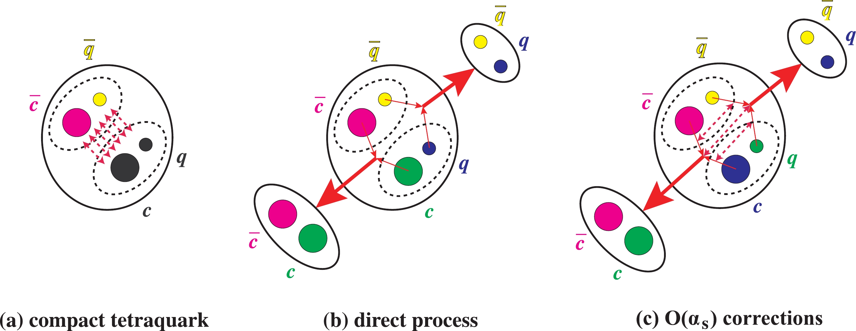 Figure2. (color online) The decay of a compact tetraquark (diquark-antidiquark) state into one charmonium meson and one light meson. This decay can happen through either (b) a direct fall-apart process, or (c) a process with gluon(s) exchanged, that is the
 $ \begin{split} [u(x) c(x)]\; [\bar d(y) \bar c(y)] \Longrightarrow & [u(x \to y^{\prime})\; c(x \to x^{\prime})]\\&\times [\bar d(y \to y^{\prime})\; \bar c(y \to x^{\prime})] \\ \Longrightarrow & [\bar c(x^{\prime}) c(x^{\prime})] + [\bar d(y^{\prime}) u(y^{\prime})] \, .\end{split} $  | (41) |
$ \begin{split} \eta^{{\cal{Z}}}_{\mu}(x,y) & \Longrightarrow + {1\over3}\; \theta_{\mu}^1(x^{\prime},y^{\prime}) - {1\over3}\; \theta_{\mu}^2(x^{\prime},y^{\prime}) \\& \;\;\;\;\;\;\;\; + {{\rm i}\over3}\; \theta_{\mu}^3(x^{\prime},y^{\prime}) - {{\rm i}\over3}\; \theta_{\mu}^4(x^{\prime},y^{\prime}) + \cdots \\& \;\;\;\;= - {{\rm i}\over3}\; I^{P}(x^{\prime}) \; J^{V}_{\mu}(y^{\prime}) + {{\rm i}\over3}\; I^{V}_{\mu}(x^{\prime}) \; J^{P}(y^{\prime}) \\& \;\;\;\;\;\;\;\; + {{\rm i}\over3}\; I^{A,\nu}(x^{\prime}) \; J^{T}_{\mu\nu}(y^{\prime}) - {{\rm i}\over3}\; I^{T}_{\mu\nu}(x^{\prime}) \; J^{A,\nu}(y^{\prime}) + \cdots \, , \end{split} $  | (42) |
Together with Table 2, we extract the following decay channels from the above transformation:
1. The decay of
$ \begin{split}& \langle Z_c^+(p,\epsilon) | \eta_c(p_1)\; \rho^+(p_2,\epsilon_2) \rangle \\\approx & - {{\rm i} c_1\over3}\; \lambda_{\eta_c} m_\rho f_{\rho^+}\; \epsilon \cdot \epsilon_2 \\& - {{\rm i} c_1\over3}\; f_{\eta_c} f^T_{\rho}\; (\epsilon \cdot p_2 \; \epsilon_2 \cdot p_1 - p_1 \cdot p_2\; \epsilon \cdot \epsilon_2) \\\equiv & g^S_{\eta_c \rho}\; \epsilon \cdot \epsilon_2 + g^D_{\eta_c \rho}\; (\epsilon \cdot p_2 \; \epsilon_2 \cdot p_1 - p_1 \cdot p_2\; \epsilon \cdot \epsilon_2) \, , \end{split} $  | (43) |
$ {\cal{L}}^S_{\eta_c \rho} = g^S_{\eta_c \rho}\; Z_{c}^{+,\mu}\; \eta_c\; \rho^{-}_{\mu} + \cdots \, , $  | (44) |
$ \begin{split}\quad\quad {\cal{L}}^D_{\eta_c \rho} =& g^D_{\eta_c \rho} \times \left( g^{\mu\sigma}g^{\nu\rho} - g^{\mu\nu}g^{\rho\sigma} \right) \\&\times Z_{c,\mu}^{+}\; \partial_\rho \eta_c\; \partial_\sigma \rho^{-}_{\nu} + \cdots \, . \end{split} $  | (45) |
$ \begin{split}& \langle Z_c^+(p,\epsilon) | J/\psi(p_1,\epsilon_1)\; \pi^+(p_2) \rangle \\ \approx & {{\rm i} c_1 \over3}\; \lambda_{\pi} m_{J/\psi} f_{J/\psi}\; \epsilon \cdot \epsilon_1 \\&+ {{\rm i} c_1 \over3}\; f_{\pi^+} f^T_{J/\psi}\; (\epsilon \cdot p_1 \; \epsilon_1 \cdot p_2 - p_1 \cdot p_2\; \epsilon \cdot \epsilon_1) \\\equiv & g^S_{\psi \pi}\; \epsilon \cdot \epsilon_1 + g^D_{\psi \pi}\; (\epsilon \cdot p_1 \; \epsilon_1 \cdot p_2 - p_1 \cdot p_2\; \epsilon \cdot \epsilon_1) \, . \end{split} $  | (46) |
$ {\cal{L}}^S_{\psi \pi} = g^S_{\psi \pi}\; Z_{c}^{+,\mu}\; \psi_{\mu}\; \pi^- + \cdots \, , $  | (47) |
$ \begin{split}{\cal{L}}^D_{\psi \pi} = g^D_{\psi \pi} \times \left( g^{\mu\rho}g^{\nu\sigma} - g^{\mu\nu}g^{\rho\sigma} \right) \times Z_{c,\mu}^{+}\; \partial_\rho \psi_\nu\; \partial_\sigma \pi^- + \cdots \, .\quad\quad \end{split} $  | (48) |
$ \begin{split}\langle Z_c^+(p,\epsilon) | \eta_c(p_1)\; b_1^+(p_2,\epsilon_2) \rangle &\approx - {{\rm i} c_1 \over3}\; f_{\eta_c} f^T_{b_1}\; \epsilon_{\mu\nu\alpha\beta} \epsilon^\mu p_1^\nu \epsilon_2^\alpha p_2^\beta \\&\equiv g_{\eta_c b_1}\; \epsilon_{\mu\nu\alpha\beta} \epsilon^\mu p_1^\nu \epsilon_2^\alpha p_2^\beta \, . \end{split} $  | (49) |
4. The decay of
$ \begin{split}&\;\;\;\;\;\; \langle Z_c^+(p,\epsilon) | \chi_{c1}(p_1,\epsilon_1)\; \rho^+(p_2,\epsilon_2) \rangle \\&\approx - {c_1\over3}\; m_{\chi_{c1}} f_{\chi_{c1}} f^T_{\rho}\; (\epsilon_1 \cdot \epsilon_2\; \epsilon \cdot p_2 - \epsilon_1 \cdot p_2\; \epsilon \cdot \epsilon_2) \\&\equiv g_{\chi_{c1} \rho}\; (\epsilon_1 \cdot \epsilon_2\; \epsilon \cdot p_2 - \epsilon_1 \cdot p_2\; \epsilon \cdot \epsilon_2) \, . \end{split} $  | (50) |
5. The decay of
$ \begin{split} &\;\;\;\;\;\; \langle Z_c^+(p,\epsilon) | \chi_{c1}(p_1,\epsilon_1)\; b_1^+(p_2,\epsilon_2) \rangle \\&\approx - {c_1\over3}\; m_{\chi_{c1}} f_{\chi_{c1}} f^T_{b_1}\; \epsilon_{\mu\nu\alpha\beta} \epsilon^\mu \epsilon_1^\nu \epsilon_2^\alpha p_2^\beta \\&\equiv g_{\chi_{c1} b_1}\; \epsilon_{\mu\nu\alpha\beta} \epsilon^\mu \epsilon_1^\nu \epsilon_2^\alpha p_2^\beta \, . \end{split} $  | (51) |
6. The decay of
$ \begin{split}&\;\;\;\;\;\; \langle Z_c^+(p,\epsilon) | h_c(p_1,\epsilon_1)\; \pi^+(p_2) \rangle \\&\approx {{\rm i} c_1\over3}\; f_{\pi^+} f^T_{h_c}\; \epsilon_{\mu\nu\alpha\beta} \epsilon^\mu p_2^\nu \epsilon_1^\alpha p_1^\beta \\&\equiv g_{h_c \pi}\; \epsilon_{\mu\nu\alpha\beta} \epsilon^\mu p_2^\nu \epsilon_1^\alpha p_1^\beta \, . \end{split} $  | (52) |
7. The decay of
$ \begin{split}&\;\;\;\;\; \langle Z_c^+(p,\epsilon) | J/\psi(p_1,\epsilon_1)\; a_1^+(p_2,\epsilon_2) \rangle \\&\approx {c_1\over3}\; f^T_{J/\psi} m_{a_1} f_{a_1}\; (\epsilon_1 \cdot \epsilon_2\; \epsilon \cdot p_1 - \epsilon_2 \cdot p_1\; \epsilon \cdot \epsilon_1) \\&\equiv g_{\psi a_1}\; (\epsilon_1 \cdot \epsilon_2\; \epsilon \cdot p_1 - \epsilon_2 \cdot p_1\; \epsilon \cdot \epsilon_1) \, . \end{split} $  | (53) |
8. The decay of
$ \begin{split}&\;\;\;\;\;\langle Z_c^+(p,\epsilon) | h_c(p_1,\epsilon_1)\; a_1^+(p_2,\epsilon_2) \rangle \\&\approx {c_1\over3}\; f^T_{h_c} m_{a_1} f_{a_1}\; \epsilon_{\mu\nu\alpha\beta} \epsilon^\mu \epsilon_2^\nu \epsilon_1^\alpha p_1^\beta \\&\equiv g_{h_c a_1}\; \epsilon_{\mu\nu\alpha\beta} \epsilon^\mu \epsilon_2^\nu \epsilon_1^\alpha p_1^\beta \, . \end{split} $  | (54) |
Summarizing the above results, we numerically obtain
$ \begin{split}& g^S_{\eta_c \rho} = - {\rm i} c_1\; 7.29 \times 10^{10}\; {\rm{MeV}}^4 \, , \\ & g^D_{\eta_c \rho} = - {\rm i} c_1\; 2.05 \times 10^{4}\; {\rm{MeV}}^2 \, , \\ & g^S_{\psi \pi} = {\rm i} c_1\; 11.87 \times 10^{10}\; {\rm{MeV}}^4 \, , \\ & g^D_{\psi \pi} = {\rm i} c_1\; 1.78 \times 10^{4}\; {\rm{MeV}}^2 \, , \\ & g_{\eta_{c} b_1} = - {\rm i} c_1\; 2.32 \times 10^{4}\; {\rm{MeV}}^2 \, , \\ & g_{\chi_{c1} \rho} = - c_1\; 6.23 \times 10^{7}\; {\rm{MeV}}^3 \, , \\ & g_{\chi_{c1} b_1} = - c_1\; 7.06 \times 10^{7}\; {\rm{MeV}}^3 \, , \\ & g_{h_c \pi} = {\rm i} c_1\; 1.02 \times 10^{4}\; {\rm{MeV}}^2 \, , \\ & g_{\psi a_1} = c_1\; 4.27 \times 10^{7}\; {\rm{MeV}}^3 \, , \\ & g_{h_c a_1} = c_1\; 2.45 \times 10^{7}\; {\rm{MeV}}^3 \, . \end{split} $  | (55) |
$ \begin{split} &{{\cal{B}}(|0_{qc}1_{\bar q \bar c} ; 1^{+-} \rangle \rightarrow \eta_c\rho) \over {\cal{B}}(|0_{qc}1_{\bar q \bar c} ; 1^{+-} \rangle \rightarrow J/\psi\pi)} = 0.059 \, , \\ & {{\cal{B}}(|0_{qc}1_{\bar q \bar c} ; 1^{+-} \rangle \rightarrow h_c\pi) \over {\cal{B}}(|0_{qc}1_{\bar q \bar c} ; 1^{+-} \rangle \rightarrow J/\psi\pi)} = 0.0088 \, , \\& {{\cal{B}}(|0_{qc}1_{\bar q \bar c} ; 1^{+-} \rangle \rightarrow \chi_{c1}\rho \rightarrow \chi_{c1}\pi \pi) \over {\cal{B}}(|0_{qc}1_{\bar q \bar c} ; 1^{+-} \rangle \rightarrow J/\psi\pi)} = 1.4 \times 10^{-6} \, . \end{split} $  | (56) |
$ \begin{split}& |0_{qc}1_{\bar q \bar c} ; 1^{+-} \rangle \rightarrow \eta_c b_1 \rightarrow \eta_c \omega \pi \rightarrow \eta_c + 4 \pi \, , \\ & |0_{qc}1_{\bar q \bar c} ; 1^{+-} \rangle \rightarrow J/\psi a_1 \rightarrow J/\psi \rho \pi \rightarrow J/\psi + 3 \pi \, . \end{split} $  | (57) |
2
4.2.$ \eta^{{\cal{Z}}}_{\mu}\big([uc][\bar d \bar c]\big) \rightarrow \xi_{\mu}^i \big([\bar c u] + [\bar d c]\big) $![]()
![]()
As depicted in Fig. 3, when the c and 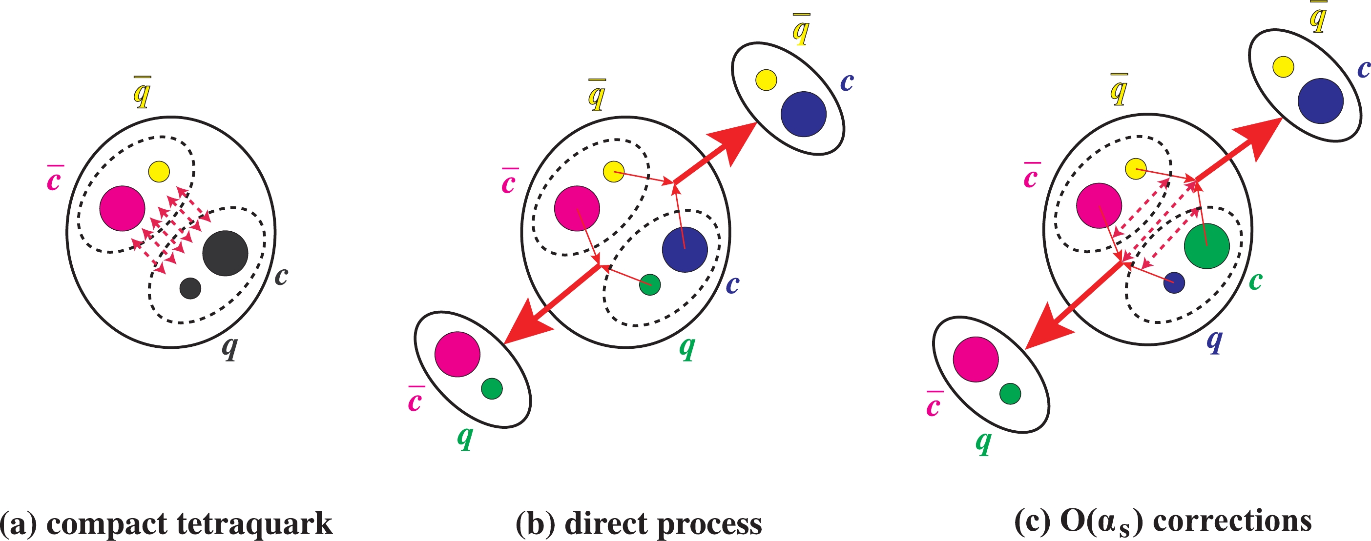 Figure3. (color online) The decay of a compact tetraquark (diquark-antidiquark) state into two charmed mesons. This decay can happen through either (b) a direct fall-apart process, or (c) a process with gluon(s) exchanged, that is the
 $ \eta^{{\cal{Z}}}_{\mu}(x,y) \Longrightarrow - {{\rm i}\over3}\; \xi_{\mu}^2(x^{\prime},y^{\prime}) + {1\over3}\; \xi_{\mu}^3(x^{\prime},y^{\prime}) + \cdots \, . $  | (58) |
The term
$ \begin{split} \langle Z_c^+(p,\epsilon) | \bar D^0(p_1)D_0^{*+}(p_2) \rangle \approx & \dfrac{{\rm i} c_2}{3}\; f_D m_{D_0^*} f_{D_0^*}\; \epsilon \cdot p_1 \\ \equiv & g_{D \bar D_0^*}\; \epsilon \cdot p_1 \, , \end{split} $  | (59) |
$ \begin{split}\langle Z_c^+(p,\epsilon) | D^+(p_1)\bar D_0^{*0}(p_2) \rangle &\approx- \dfrac{{\rm i} c_2}{3}\; f_D m_{D_0^*} f_{D_0^*}\; \epsilon \cdot p_1\\ &\equiv - g_{D \bar D_0^*}\; \epsilon \cdot p_1 \, , \end{split} $  | (60) |
Thus, we numerically obtain
$ g_{D \bar D_0^*} = {\rm i}c_2\; 6.80 \times 10^{7}\; {\rm{MeV}}^3 \, . $  | (61) |
$ {{\cal{B}}(|0_{qc}1_{\bar q \bar c} ; 1^{+-} \rangle \rightarrow D \bar D_0^{*} + \bar D D_0^{*} \rightarrow D \bar D \pi) \over {\cal{B}}(|0_{qc}1_{\bar q \bar c} ; 1^{+-} \rangle \rightarrow J/\psi\pi+ \eta_c\rho)} = 9.3 \times 10^{-8} \times {c_2^2 \over c_1^2} \, . $  | (62) |
$ g_{D \bar D^{*}} \approx 0 \, , $  | (63) |
$ {{\cal{B}}(|0_{qc}1_{\bar q \bar c} ; 1^{+-} \rangle \rightarrow D \bar D^{*} + \bar D D^{*}) \over {\cal{B}}(|0_{qc}1_{\bar q \bar c} ; 1^{+-} \rangle \rightarrow J/\psi\pi + \eta_c\rho)} \approx 0 \, . $  | (64) |
2
4.3.$ \eta^{{\cal{Z}}}_{\mu}\big([uc][\bar d \bar c]\big) \rightarrow \theta_{\mu}^{1,2,3,4}\big([\bar c c] + [\bar d u]\big) + \xi_{\mu}^{1,2,3,4}\big([\bar c u] + [\bar d c]\big) $![]()
![]()
If the above two processes investigated in Sec. 4.1 and Sec. 4.2 happen at the same time, we can use the transformation (18); i.e., $ \begin{split} \eta^{{\cal{Z}}}_{\mu}(x,y) \Longrightarrow & + {1\over2}\; \theta_{\mu}^1(x^{\prime},y^{\prime}) - {1\over2}\; \theta_{\mu}^2(x^{\prime},y^{\prime}) + {{\rm i}\over2}\; \theta_{\mu}^3(x^{\prime},y^{\prime}) \\ & - {{\rm i}\over2}\; \theta_{\mu}^4(x^{\prime},y^{\prime}) - {{\rm i}\over2}\; \xi_{\mu}^2(x^{\prime\prime},y^{\prime\prime}) + {1\over2}\; \xi_{\mu}^3(x^{\prime\prime},y^{\prime\prime}) \, . \end{split} $  | (65) |
Comparing the above equation with Eqs. (42) and (58), we obtain the same relative branching ratios as Sec. 4.1 and Sec. 4.2, with just the overall factors
2
4.4.Mixing with $ |1_{qc}1_{\bar q \bar c} ; 1^{+-} \rangle $![]()
![]()
The relative branching ratio Actually, in the Type-II diquark-antidiquark model [6], the
$ |0_{qc}1_{\bar q \bar c} ; 1^{+-} \rangle = {1\over\sqrt2} \left(| 0_{qc}, 1_{\bar q \bar c} \rangle_{J = 1} - |1_{qc}, 0_{\bar q \bar c} \rangle_{J = 1} \right) \, , $  |
$ |x_{qc}1_{\bar q \bar c} ; 1^{+-} \rangle = \cos \theta_1 \; |0_{qc}1_{\bar q \bar c} ; 1^{+-} \rangle + \sin \theta_1 \; |1_{qc}1_{\bar q \bar c} ; 1^{+-} \rangle \, , $  | (66) |
$ |1_{qc}1_{\bar q \bar c} ; 1^{+-} \rangle = | 1_{qc}, 1_{\bar q \bar c} \rangle_{J = 1} \, , $  | (67) |
Thus, we attempt to add this
$ \eta^{{\cal{Z}}^{\prime}}_{\mu}(x,y) = \eta^3_{\mu}([uc][\bar d \bar c]) - \eta^4_{\mu}([uc][\bar d \bar c]) \, , $  | (68) |
$ \eta^{\rm{mix}}_{\mu}(x,y) = \cos \theta^{\prime}_1\; \eta^{{\cal{Z}}}_{\mu}(x,y) + {\rm i} \sin \theta^{\prime}_1\; \eta^{{\cal{Z}}^{\prime}}_{\mu}(x,y)\, , $  | (69) |
$ \begin{split} \eta^{\rm{mix}}_{\mu}(x,y) \Longrightarrow & + \left( -{{\rm i}\over3} \cos \theta^{\prime}_1 + {\rm i} \sin \theta^{\prime}_1 \right) \; I^{P}(x^{\prime}) \; J^{V}_{\mu}(y^{\prime}) \\ & + \left( + {{\rm i}\over3} \cos \theta^{\prime}_1 + {\rm i} \sin \theta^{\prime}_1 \right) \; I^{V}_{\mu}(x^{\prime}) \; J^{P}(y^{\prime}) \\ & + \left( + {{\rm i}\over3} \cos \theta^{\prime}_1 - {{\rm i}\over3} \sin \theta^{\prime}_1 \right) \; I^{A,\nu}(x^{\prime}) \; J^{T}_{\mu\nu}(y^{\prime}) \\ & + \left( - {{\rm i}\over3} \cos \theta^{\prime}_1 - {{\rm i}\over3} \sin \theta^{\prime}_1 \right) \; I^{T}_{\mu\nu}(x^{\prime}) \; J^{A,\nu}(y^{\prime}) + \cdots \, . \end{split} $  | (70) |
$ \theta_1 = f(\theta^{\prime}_1) \, . $  | (71) |
$ \begin{split} & {\cal{R}}_{\psi \pi} \equiv {\Gamma(|x_{qc}1_{\bar q \bar c} ; 1^{+-} \rangle \rightarrow J/\psi\pi) \over \Gamma(|0_{qc}1_{\bar q \bar c} ; 1^{+-} \rangle \rightarrow J/\psi\pi)} \, , \\ & {\cal{R}}_{\eta_c \rho} \equiv {\Gamma(|x_{qc}1_{\bar q \bar c} ; 1^{+-} \rangle \rightarrow \eta_c \rho) \over \Gamma(|0_{qc}1_{\bar q \bar c} ; 1^{+-} \rangle \rightarrow \eta_c \rho)} \, , \\ & {\cal{R}} \equiv {{\cal{B}}(|x_{qc}1_{\bar q \bar c} ; 1^{+-} \rangle \rightarrow \eta_c\rho) \over {\cal{B}}(|x_{qc}1_{\bar q \bar c} ; 1^{+-} \rangle \rightarrow J/\psi\pi)} \, , \end{split} $  | (72) |
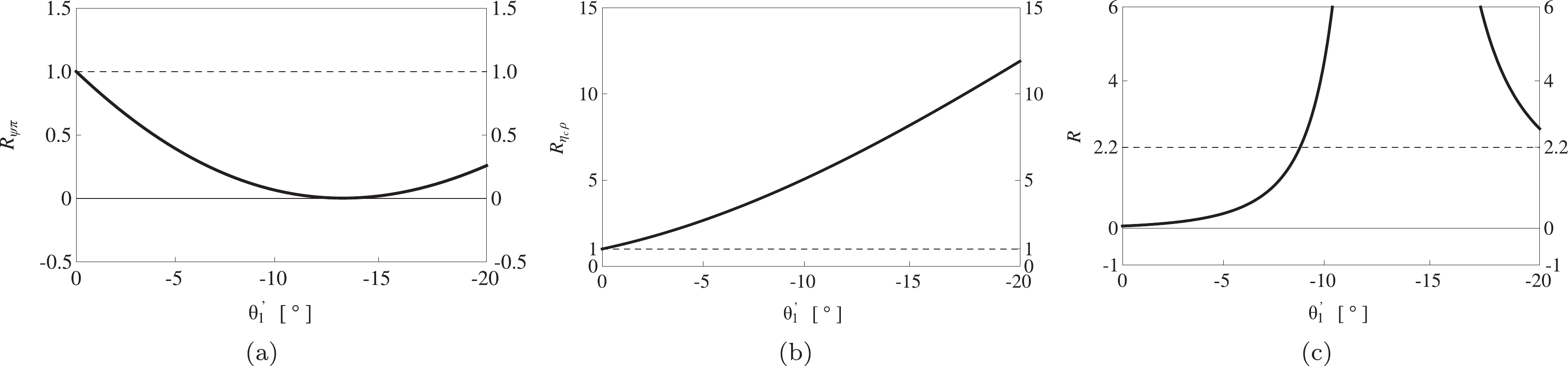 Figure4. The ratios (a)
 Especially, after fine-tuning
$ \begin{split} {\cal{R}} \equiv & \dfrac{{\cal{B}}(|x_{qc}1_{\bar q \bar c} ; 1^{+-} \rangle \rightarrow \eta_c\rho) }{ {\cal{B}}(|x_{qc}1_{\bar q \bar c} ; 1^{+-} \rangle \rightarrow J/\psi\pi)} = 2.2 \, , \\& \dfrac{{\cal{B}}(|x_{qc}1_{\bar q \bar c} ; 1^{+-} \rangle \rightarrow h_c\pi) }{ {\cal{B}}(|x_{qc}1_{\bar q \bar c} ; 1^{+-} \rangle \rightarrow J/\psi\pi)} = 0.052 \, , \\ & \dfrac{{\cal{B}}(|x_{qc}1_{\bar q \bar c} ; 1^{+-} \rangle \rightarrow \chi_{c1}\rho \rightarrow \chi_{c1} \pi \pi)}{{\cal{B}}(|x_{qc}1_{\bar q \bar c} ; 1^{+-} \rangle \rightarrow J/\psi\pi)} = 1.5 \times 10^{-5} \, . \end{split} $  | (73) |
The decay of
$ \begin{split} \eta^{\rm{mix}}_{\mu}(x,y) \Longrightarrow & - {{\rm i}\over3}\; \cos \theta^{\prime}_1\; \xi_{\mu}^2(x^{\prime},y^{\prime}) + {1\over3}\; \cos \theta^{\prime}_1\; \xi_{\mu}^3(x^{\prime},y^{\prime}) \\ & -\; \sin \theta^{\prime}_1\; \xi_{\mu}^1(x^{\prime},y^{\prime}) - {{\rm i}\over3}\; \sin \theta^{\prime}_1\; \xi_{\mu}^4(x^{\prime},y^{\prime}) + \cdots \, , \end{split} $  | (74) |
$ \begin{split}& \dfrac{{\cal{B}}(|x_{qc}1_{\bar q \bar c} ; 1^{+-} \rangle \rightarrow D \bar D^{*} + \bar D D^{*}) }{ {\cal{B}}(|x_{qc}1_{\bar q \bar c} ; 1^{+-} \rangle \rightarrow J/\psi\pi + \eta_c\rho)} = 0.26 \times \dfrac{c_2^2}{ c_1^2} \, , \\&\dfrac{{\cal{B}}(|x_{qc}1_{\bar q \bar c} ; 1^{+-} \rangle \rightarrow D \bar D_0^{*} + \bar D D_0^{*} \rightarrow D \bar D \pi) }{ {\cal{B}}(|x_{qc}1_{\bar q \bar c} ; 1^{+-} \rangle \rightarrow J/\psi\pi + \eta_c\rho)} = 2.5 \times 10^{-7} \times \dfrac{c_2^2 }{ c_1^2} \, . \end{split} $  | (75) |
2
5.1.$ \xi^{{\cal{Z}}}_{\mu}\big([\bar c u][\bar d c]\big) \longrightarrow \theta_{\mu}^{i}\big([\bar c c] + [\bar d u]\big) $![]()
![]()
As depicted in Fig. 5, when the c and 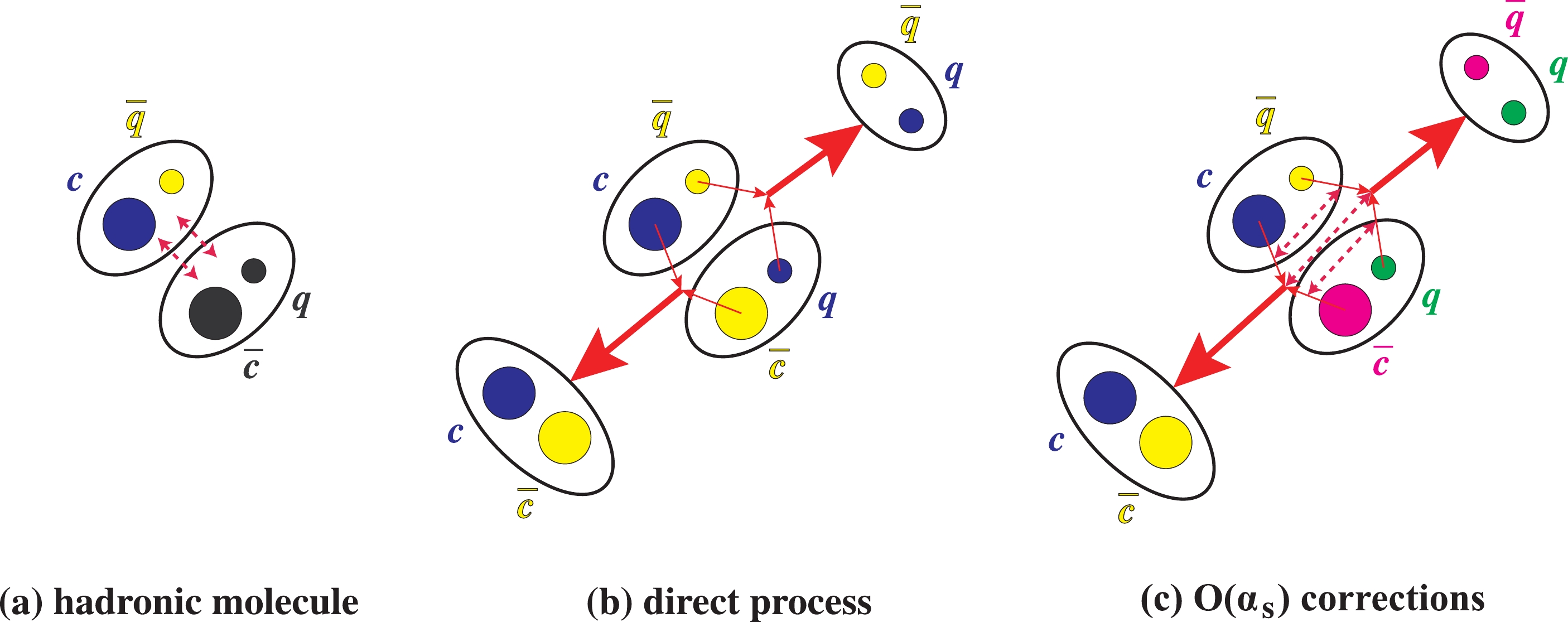 Figure5. (color online) The decay of a hadronic molecular state into one charmonium meson and one light meson. This decay can happen through either (b) a direct fall-apart process, or (c) a process with gluon(s) exchanged, that is the
 $ \begin{split} \xi^{{\cal{Z}}}_{\mu}(x,y) \Longrightarrow& -\dfrac{1}{6}\; \theta_{\mu}^1(x^{\prime},y^{\prime}) - {1\over6}\; \theta_{\mu}^2(x^{\prime},y^{\prime}) - \dfrac{{\rm i}}{6}\; \theta_{\mu}^3(x^{\prime},y^{\prime})\\ & - {{\rm i}\over6}\; \theta_{\mu}^4(x^{\prime},y^{\prime}) + \cdots = + {{\rm i}\over6}\; I^{P}(x^{\prime}) \; J^{V}_{\mu}(y^{\prime}) \\ &+ {{\rm i}\over6}\; I^{V}_{\mu}(x^{\prime}) \; J^{P}(y^{\prime}) - \dfrac{{\rm i}}{6}\; I^{A,\nu}(x^{\prime}) \; J^{T}_{\mu\nu}(y^{\prime}) \\ &- \dfrac{{\rm i}}{6}\; I^{T}_{\mu\nu}(x^{\prime}) \; J^{A,\nu}(y^{\prime}) + \cdots \, , \end{split} $  | (76) |
We repeat the same procedures as those performed in Sec. 4.1, and extract the following coupling constants from this transformation:
$ \begin{split} & h^S_{\eta_c \rho} = \dfrac{{\rm i} c_4}{ 6} \lambda_{\eta_c} m_\rho f_{\rho^+} = {\rm i} c_4\; 3.65 \times 10^{10}\; {\rm{MeV}}^4 \, , \\[-1pt]& h^D_{\eta_c \rho} = \dfrac{{\rm i} c_4}{ 6} f_{\eta_c} f^T_{\rho} = {\rm i} c_4\; 1.03 \times 10^{4}\; {\rm{MeV}}^2 \, , \\[-1pt]& h^S_{\psi \pi} = \dfrac{{\rm i} c_4}{ 6} \lambda_{\pi} m_{J/\psi} f_{J/\psi} ={\rm i} c_4\; 5.93 \times 10^{10}\; {\rm{MeV}}^4 \, , \\[-1pt]& h^D_{\psi \pi} = \dfrac{{\rm i} c_4 }{ 6} f_{\pi^+} f^T_{J/\psi} = {\rm i} c_4\; 0.89 \times 10^{4}\; {\rm{MeV}}^2 \, , \\[-1pt]& h_{\eta_c b_1} = \dfrac{{\rm i} c_4}{ 6} f_{\eta_c} f^T_{b_1} = {\rm i} c_4\; 1.16 \times 10^{4}\; {\rm{MeV}}^2 \, , \\[-1pt]& h_{\chi_{c1} \rho} = \dfrac{c_4}{ 6} m_{\chi_{c1}} f_{\chi_{c1}} f^T_{\rho} = c_4\; 3.12 \times 10^{7}\; {\rm{MeV}}^3 \, , \\[-1pt] & h_{\chi_{c1} b_1} = \dfrac{c_4}{ 6} m_{\chi_{c1}} f_{\chi_{c1}} f^T_{b_1} = c_4\; 3.53 \times 10^{7}\; {\rm{MeV}}^3 \, , \\[-1pt]& h_{h_c \pi} = \dfrac{{\rm i} c_4}{ 6} f_{\pi^+} f^T_{h_c} = {\rm i} c_4\; 0.51 \times 10^{4}\; {\rm{MeV}}^2 \, , \\[-1pt] & h_{\psi a_1} = \dfrac{c_4}{ 6} f^T_{J/\psi} m_{a_1} f_{a_1} = c_4\; 2.13 \times 10^{7}\; {\rm{MeV}}^3 \, , \\[-1pt] & h_{h_c a_1} = \dfrac{c_4}{ 6} f^T_{h_c} m_{a_1} f_{a_1} = c_4\; 1.22 \times 10^{7}\; {\rm{MeV}}^3 \, . \end{split} $  | (77) |
Using the above coupling constants, we further obtain
$ \begin{split} & {{\cal{B}}(| D \bar D^*; 1^{+-} \rangle \rightarrow \eta_c\rho) \over {\cal{B}}(| D \bar D^*; 1^{+-} \rangle \rightarrow J/\psi\pi)} = 0.059 \, , \\& {{\cal{B}}(| D \bar D^*; 1^{+-} \rangle \rightarrow h_c\pi) \over {\cal{B}}(| D \bar D^*; 1^{+-} \rangle \rightarrow J/\psi\pi)} = 0.0088 \, , \\ & {{\cal{B}}(| D \bar D^*; 1^{+-} \rangle \rightarrow \chi_{c1}\rho \rightarrow \chi_{c1}\pi \pi) \over {\cal{B}}(| D \bar D^*; 1^{+-} \rangle \rightarrow J/\psi\pi)} = 1.4 \times 10^{-6} \, . \end{split} $  | (78) |
2
5.2.$ \xi^{{\cal{Z}}}_{\mu}\big([\bar c u][\bar d c]\big) \longrightarrow \xi^i_{\mu}\big([\bar c u] + [\bar d c]\big) $![]()
![]()
Assuming the $ \xi^{{\cal{Z}}}_{\mu}(x,y) \Longrightarrow \xi_{\mu}^1(x^{\prime},y^{\prime}) = -{\rm i}\; O^{V}_{\mu}(x^{\prime}) \; O^{P}(y^{\prime}) + \{ \gamma_{\mu} \leftrightarrow \gamma_5 \} \, . $  | (79) |
$ \begin{split}\langle Z_c^+(p,\epsilon) | D^+(p_1) \bar D^{*0}(p_2,\epsilon_2) \rangle \approx &-{\rm i}c_5\; \lambda_D m_{D^*} f_{D^*}\; \epsilon \cdot \epsilon_2 \\ & \equiv h_{D \bar D^*}\; \epsilon \cdot \epsilon_2 \, , \end{split} $  | (80) |
$ \begin{split} \langle Z_c^+(p,\epsilon) | \bar D^0(p_1) D^{*+}(p_2,\epsilon_2) \rangle \approx & -{\rm i}c_5\; \lambda_D m_{D^*} f_{D^*}\; \epsilon \cdot \epsilon_2 \\& \equiv h_{D \bar D^*}\; \epsilon \cdot \epsilon_2 \, , \end{split} $  | (81) |
$ h_{D \bar D^*} = -{\rm i}c_5\; 2.95 \times 10^{11}\; {\rm{MeV}}^4 \, . $  | (82) |
$ {{\cal{B}}(| D \bar D^*; 1^{+-} \rangle \rightarrow D \bar D^{*} + \bar D D^{*}) \over {\cal{B}}(| D \bar D^*; 1^{+-} \rangle \rightarrow J/\psi\pi + \eta_c\rho)} = 25 \times {c_5^2 \over c_4^2} \, . $  | (83) |
$ {{\cal{B}}(| D \bar D^*; 1^{+-} \rangle \rightarrow D \bar D_0^{*} + \bar D D_0^{*} \rightarrow D \bar D \pi) \over {\cal{B}}(| D \bar D^*; 1^{+-} \rangle \rightarrow J/\psi\pi + \eta_c\rho)} \approx 0 \, . $  | (84) |
2
5.3.Mixing with the $ | D^* \bar D^*; 1^{+-} \rangle $![]()
![]()
Similarly to Sec. 4.4, we add a small $ | D^* \bar D^*; 1^{+-} \rangle = | D^* \bar D^* \rangle_{J = 1} \, , $  | (85) |
$ \xi^{{\cal{Z}}^{\prime}}_{\mu}(x,y) = \xi^2_{\mu}([\bar c u][\bar d c]) \, , $  | (86) |
$ \xi^{\rm{mix}}_{\mu}(x,y) = \cos \theta^{\prime}_2\; \xi^{{\cal{Z}}}_{\mu}(x,y) + {\rm i} \sin \theta^{\prime}_2\; \xi^{{\cal{Z}}^{\prime}}_{\mu}(x,y) \, , $  | (87) |
$ |D^{(*)} \bar D^*; 1^{+-} \rangle = \cos \theta_2 \; |D \bar D^*; 1^{+-} \rangle + \sin \theta_2 \; |D^* \bar D^*; 1^{+-} \rangle \, . $  | (88) |
$ \begin{split} \xi^{\rm{mix}}_{\mu}(x,y) \Longrightarrow & + \left( + {{\rm i}\over6}\cos \theta^{\prime}_2 - {{\rm i}\over2}\sin \theta^{\prime}_2 \right) \; I^{P}(x^{\prime}) \; J^{V}_{\mu}(y^{\prime}) \\ & + \left( + {{\rm i}\over6}\cos \theta^{\prime}_2 + {{\rm i}\over2} \sin \theta^{\prime}_2 \right) \; I^{V}_{\mu}(x^{\prime}) \; J^{P}(y^{\prime}) \\ &+ \left( - {{\rm i}\over6}\cos \theta^{\prime}_2 + {{\rm i}\over6} \sin \theta^{\prime}_2 \right) \; I^{A,\nu}(x^{\prime}) \; J^{T}_{\mu\nu}(y^{\prime}) \\ &+ \left( - {{\rm i}\over6}\cos \theta^{\prime}_2 - {{\rm i}\over6} \sin \theta^{\prime}_2 \right) \; I^{T}_{\mu\nu}(x^{\prime}) \; J^{A,\nu}(y^{\prime}) + \cdots \, . \end{split} $  | (89) |
$ \begin{split} {\cal{R}}^{\prime} \equiv & {{\cal{B}}(|D^{(*)} \bar D^*; 1^{+-} \rangle \rightarrow \eta_c\rho) \over {\cal{B}}(|D^{(*)} \bar D^*; 1^{+-} \rangle \rightarrow J/\psi\pi)} = 2.2 \, , \\ & {{\cal{B}}(|D^{(*)} \bar D^*; 1^{+-} \rangle \rightarrow h_c\pi) \over {\cal{B}}(|D^{(*)} \bar D^*; 1^{+-} \rangle \rightarrow J/\psi\pi)} = 0.052 \, , \\ &{{\cal{B}}(|D^{(*)} \bar D^*; 1^{+-} \rangle \rightarrow \chi_{c1}\rho \rightarrow \chi_{c1} \pi \pi) \over {\cal{B}}(|D^{(*)} \bar D^*; 1^{+-} \rangle \rightarrow J/\psi\pi)} = 1.5 \times 10^{-5} \, , \end{split} $  | (90) |
$ \begin{split} & {\cal{R}}^{\prime}_{\psi \pi} \equiv {\Gamma(|D^{(*)} \bar D^*; 1^{+-} \rangle \rightarrow J/\psi\pi) \over \Gamma(|D \bar D^*; 1^{+-} \rangle \rightarrow J/\psi\pi)} \, , \\ &{\cal{R}}^{\prime}_{\eta_c \rho} \equiv {\Gamma(|D^{(*)} \bar D^*; 1^{+-} \rangle \rightarrow \eta_c \rho) \over \Gamma(|D \bar D^*; 1^{+-} \rangle \rightarrow \eta_c \rho)} \, , \\ & {\cal{R}}^{\prime} \equiv {{\cal{B}}(|D^{(*)} \bar D^*; 1^{+-} \rangle \rightarrow \eta_c \rho) \over {\cal{B}}(|D^{(*)} \bar D^*; 1^{+-} \rangle \rightarrow J/\psi\pi)} \, , \end{split} $  | (91) |
We also obtain
$ \begin{split} & {{\cal{B}}(|D^{(*)} \bar D^*; 1^{+-} \rangle \rightarrow D \bar D^{*} + \bar D D^{*}) \over {\cal{B}}(|D^{(*)} \bar D^*; 1^{+-} \rangle \rightarrow J/\psi\pi + \eta_c\rho)} = 67 \times {c_5^2 \over c_4^2} \, , \\ &{{\cal{B}}(|D^{(*)} \bar D^*; 1^{+-} \rangle \rightarrow D \bar D_0^{*} + \bar D D_0^{*} \rightarrow D \bar D \pi) \over {\cal{B}}(|D^{(*)} \bar D^*; 1^{+-} \rangle \rightarrow J/\psi\pi + \eta_c\rho)} \approx 0 \, , \end{split} $  | (92) |
● Using the transformation of
● Using the transformation of
● We use the transformation of the
● Using the transformation of
● Through the
Our results suggest that the possible decay channels of the
| channels |   |     |   |     |
  |   |   |   |   |
  |   |   |   |   |
  |   |   |   |   |
  |   |   |   |   |
  |   |   |   |   |
Table3.Relative branching ratios of the
● In the second and third columns of Table 3,
$ | 0_{qc}1_{\bar q \bar c}; 1^{+-} \rangle \oplus | 1_{qc}1_{\bar q \bar c}; 1^{+-} \rangle \rightarrow | x_{qc}1_{\bar q \bar c}; 1^{+-} \rangle \, . $  | (93) |
$ \begin{split} {{\cal{B}}\left(| x_{qc}1_{\bar q \bar c}; 1^{+-} \rangle \rightarrow J/\psi\pi \!:\! \eta_c\rho \!:\! h_c\pi \!:\! \chi_{c1}\rho (\rightarrow \pi \pi) \!:\! D \bar D^{*} \!:\! D \bar D_0^{*} (\rightarrow \bar D \pi) \right) \over {\cal{B}}(| x_{qc}1_{\bar q \bar c}; 1^{+-} \rangle \rightarrow J/\psi\pi)} \approx 1 \!:\! 2.2 ({\rm{input}}) \!:\! 0.05 \!:\! 10^{-5} \!:\! 0.82 t_1 : 10^{-6} t_1 . \end{split} $  | (94) |
$ | D \bar D^*; 1^{+-} \rangle \oplus |D^{*} \bar D^*; 1^{+-} \rangle \rightarrow |D^{(*)} \bar D^*; 1^{+-} \rangle \, . $  | (95) |
$ \begin{split} &{{\cal{B}}\left(|D^{(*)} \bar D^*; 1^{+-} \rangle \rightarrow J/\psi\pi : \eta_c\rho : h_c\pi \, : \chi_{c1}\rho (\rightarrow \pi \pi) : D \bar D^{*} \right) \over {\cal{B}}(|D^{(*)} \bar D^*; 1^{+-} \rangle \rightarrow J/\psi\pi)} \\ \approx &\,1 \, : 2.2 ({\rm{input}}) : 0.05 : 10^{-5} \, : 210 t_2 \, . \end{split} $  | (96) |
The above relative branching ratios calculated in the present study turn out to be very different, which may be one of the reasons why many multiquark states were observed in only a few decay channels [75]. Note that in order to extract the above results, we have only considered the leading-order fall-apart decays described by color-singlet-color-singlet meson-meson currents but neglected the
Based on Table 3 as well as Eqs. (94) and (96), we conclude this paper:
● The relative branching ratios
● The relative branching ratios of the
●
It is useful to generally discuss our uncertainty. In this study, we have worked within the naive factorization scheme; thus, our uncertainty is greater than that of well-developed QCD factorization method [62–64], which is at 5% when being applied to study the weak and radiative decay properties of conventional (heavy) hadrons. On the other hand, the tetraquark decay constant
Next,let us compare our results with other theoretical calculations. First, we compare them with the QCD sum rule results obtained in Refs. [30, 31], where the
$ \begin{split} & {{\cal{B}}(|0_{qc}1_{\bar q \bar c} ; 1^{+-} \rangle \rightarrow \eta_c\rho)_{S{-}{\rm{wave}}} \over {\cal{B}}(|0_{qc}1_{\bar q \bar c} ; 1^{+-} \rangle \rightarrow J/\psi\pi)_{S{-}{\rm{wave}}}} = 0.24 \, , \\& {{\cal{B}}(|0_{qc}1_{\bar q \bar c} ; 1^{+-} \rangle \rightarrow \eta_c\rho)_{D{-}{\rm{wave}}} \over {\cal{B}}(|0_{qc}1_{\bar q \bar c} ; 1^{+-} \rangle \rightarrow J/\psi\pi)_{D{-}{\rm{wave}}}} = 0.82 \, . \end{split} $  | (97) |
$ \begin{split} & \Gamma(Z_c(3900) \rightarrow \eta_c\rho) = 27.5 \pm 8.5\; {\rm{MeV}} \, , \\& \Gamma(Z_c(3900) \rightarrow J/\psi\pi) = 29.1 \pm 8.2\; {\rm{MeV}} \, , \end{split} $  | (98) |
$ {{\cal{B}}(Z_c(3900) \rightarrow \eta_c\rho)_{S{-}{\rm{wave}}} \over {\cal{B}}(Z_c(3900) \rightarrow J/\psi\pi)_{S{-}{\rm{wave}}}} = 0.95^{+0.47}_{-0.36} \, . $  | (99) |
$ \begin{split}&\Gamma(Z_c(3900) \rightarrow \eta_c\rho) = 23.8 \pm 4.9\; {\rm{MeV}} \, , \\&\Gamma(Z_c(3900) \rightarrow J/\psi\pi) = 41.9 \pm 9.4\; {\rm{MeV}} \, , \end{split} $  | (100) |
$ {{\cal{B}}(Z_c(3900) \rightarrow \eta_c\rho)_{D{-}{\rm{wave}}} \over {\cal{B}}(Z_c(3900) \rightarrow J/\psi\pi)_{D{-}{\rm{wave}}}} = 0.57^{+0.20}_{-0.16} \, . $  | (101) |
$ \begin{split} & {{\cal{B}}(|0_{qc}1_{\bar q \bar c} ; 1^{+-} \rangle \rightarrow \eta_c\rho)_{D{-}{\rm{wave}}} \over {\cal{B}}(|0_{qc}1_{\bar q \bar c} ; 1^{+-} \rangle \rightarrow \eta_c\rho)_{S{-}{\rm{wave}}}} = 0.51 \, , \\ & {{\cal{B}}(|0_{qc}1_{\bar q \bar c} ; 1^{+-} \rangle \rightarrow J/\psi\pi)_{D{-}{\rm{wave}}} \over {\cal{B}}(|0_{qc}1_{\bar q \bar c} ; 1^{+-} \rangle \rightarrow J/\psi\pi)_{S{-}{\rm{wave}}}} = 0.15 \, . \end{split} $  | (102) |
Following this, we compare our results with Ref. [40], where the authors assumed the
$ {{\cal{B}}(Z_c(3900) \rightarrow \eta_c\rho) \over {\cal{B}}(Z_c(3900) \rightarrow J/\psi\pi)} = 0.046^{+0.025}_{-0.017} \, . $  | (103) |
$ {{\cal{B}}(| D \bar D^*; 1^{+-} \rangle \rightarrow \eta_c\rho) \over {\cal{B}}(| D \bar D^*; 1^{+-} \rangle \rightarrow J/\psi\pi)} = 0.059 \, . $  | (104) |
We thank Fu-Sheng Yu and Qin Chang for helpful discussions.
$ {\cal{L}}^S_{\eta_c \rho} = g^S_{\eta_c \rho}\; Z_{c}^{+,\mu}\; \eta_c\; \rho^{-}_{\mu} + \cdots \, ,\tag{A1} $  | (A1) |
$ {\cal{L}}^D_{\eta_c \rho} = g^D_{\eta_c \rho} \times \left( g^{\mu\sigma}g^{\nu\rho} - g^{\mu\nu}g^{\rho\sigma} \right) Z_{c,\mu}^{+}\; \partial_\rho \eta_c\; \partial_\sigma \rho^{-}_{\nu} + \cdots \, . \tag{A2}$  | (A2) |
$ {\cal{L}}^S_{\psi \pi} = g^S_{\psi \pi}\; Z_{c}^{+,\mu}\; \psi_{\mu}\; \pi^- + \cdots \, , \tag{A3}$  | (A3) |
$ {\cal{L}}^D_{\psi \pi} = g^D_{\psi \pi} \times \left( g^{\mu\rho}g^{\nu\sigma} - g^{\mu\nu}g^{\rho\sigma} \right) Z_{c,\mu}^{+}\; \partial_\rho \psi_\nu\; \partial_\sigma \pi^- + \cdots \, . \tag{A4} $  | (A4) |
We rotate this phase angle between all S- and D-wave coupling constants to be
| channels |   |     |   |     |
  |   |   |   |   |
  |   |   |   |   |
  |   |   |   |   |
  |   |   |   |   |
  |   |   |   |   |
TableA1.Relative branching ratios of the
$ \begin{split} {{\cal{B}}\left(| x_{qc}1_{\bar q \bar c}; 1^{+-} \rangle \rightarrow J/\psi\pi\; : \eta_c\rho : h_c\pi : \chi_{c1}\rho (\rightarrow \pi \pi) : D \bar D^{*} : D \bar D_0^{*} (\rightarrow \bar D \pi)\; \right) \over {\cal{B}}(| x_{qc}1_{\bar q \bar c}; 1^{+-} \rangle \rightarrow J/\psi\pi)} \approx \; 1 : \; 2.2\; ({\rm{input}})\; : 0.004 : 10^{-6} \; \, : 0.19\; t_1 : \; 10^{-7}\; t_1\; \, ,\end{split} \tag{{A5}}$  | (A5) |
$ \begin{split}{{\cal{B}}\left(|D^{(*)} \bar D^*; 1^{+-} \rangle \rightarrow J/\psi\pi :\; \eta_c\rho :\; h_c\pi :\; \chi_{c1}\rho (\rightarrow \pi \pi)\; :\; D \bar D^{*}\; \right) \over {\cal{B}}(|D^{(*)} \bar D^*; 1^{+-} \rangle \rightarrow J/\psi\pi)} \approx \,1 \, : 2.2 ({\rm{input}})\; : 0.004 : 10^{-6}\; \, : 16 t_2 \, . \end{split} \tag{{A6}}$  | (A6) |
