Wen Chen ^1,2,3,
, Feng Feng ^1,4,
, Yu Jia ^1,2,
, Wen-Long Sang ^5,
, 1.Institute of High Energy Physics, Chinese Academy of Science, Beijing 100049, China
2.School of Physics, University of Chinese Academy of Sciences, Beijing 100049, China
3.Department of Physics, University of Alberta, Canada
4.China University of Mining and Technology, Beijing 100083, China
5.School of Physical Science and Technology, Southwest University, Chongqing 400700, China
Received Date:2018-04-11
Available Online:2019-01-01
Abstract:The associated production of Higgs boson with a muon pair, e⁺e^? → μ⁺μ^-H, is one of the golden channels to pin down the properties of the Higgs boson in the prospective Higgs factories exemplified by CEPC. The projected accuracy of the corresponding cross section measurement is about per cent level at CEPC. In this work, we investigate both ${\mathcal{O}}(\alpha )$ weak correction and the ${\mathcal{O}}(\alpha {\alpha }_{s})$ mixed electroweak-QCD corrections for this channel, appropriately taking into account the effect of finite Z⁰ width. The μ⁺μ^- invariant mass spectrum is also predicted. The mixed electroweak-QCD correction turns out to reach 1.5% of the Born-order result, and thereby must be included in future confrontation with the data. We also observe that, after including higher-order corrections, the simplified prediction for the integrated cross section employing the narrow-width-approximation may deviate from our full result by a few per cents.

HTML

--> --> -->

Ever since the ground-breaking discovery of the Higgs boson at Large Hadron Collider (LHC) in 2012 [1, 2], one of the highest priorities of particle physics is to nail down the properties of the Higgs boson as precise as possible. Unlike the hadron colliders, which suffer from severe contamination due to the copious background events, the electron-positron colliders provide an ideal platform to precisely measure various Higgs couplings [3]. In recent years, three next-generation e⁺e^? colliders have been proposed for dedicated study of Higgs boson: International Linear Collider (ILC) [4], Future Circular Collider (FCC-ee) [5], and Circular Electron-Positron Collider (CEPC) [6], all of which plan to operate at the center-of-mass energy around 240~250 GeV.
There emerge several Higgs production mechanisms at e⁺e^? colliders: Higgsstrahlung, WW fusion and ZZ fusion, etc.. Around $\sqrt{s}\approx 240$ GeV, which is the projected energy range of CEPC, the Higgs production is dominated by the Higgsstrahlung channel e⁺e^?→ZH, Higgs production associated with a Z⁰ boson. It is anticipated that, with the aid of very high luminosity and the recoil mass technique, CEPC can measure the Higgs production cross section with an exquisite sub-per-cent accuracy. Needless to say, it is indispensable for theoretical predictions for the Higgsstrahlung channel to be commensurate with the projected experimental precision.
The leading order (LO) prediction for e⁺e^? → ZH was first considered in 70s [7-10]. In the early 90s, the next-to-leading order (NLO) electroweak correction for this process has also been addressed by three groups independently [11-13], which turns out to be significant. Very recently, the mixed electroweak-QCD next-to-next-to-leading (NNLO) corrections were also be independently calculated by two groups [14, 15]. The ${\mathcal{O}}(\alpha {\alpha }_{s})$ correction may reach 1% of the LO prediction, thereby must be included when confronting the future measurement. Recently, the ISR effect of this process has also been carefully analyzed [16].
From the experimental angle, it is the decay products of the Z⁰ boson, rather than the Z⁰ itself that are tagged by detectors in the Higgsstrahlung channel, since the Z⁰ is an unstable particle. Therefore, in order to get closer contact with experiment, it is advantageous to make precise predictions directly for the process ${e}^{+}{e}^{-}\to ({Z}^{* }\to )f\bar{f}+H$, where f represents leptons or quarks. Among a flurry of Higgs production channels associated with various Z decay products, the e⁺e^?→μ⁺μ^-H process occupies a unique place for probing Higgs properties, because it is a very clean channel and possesses large cross section. The production cross section for this individual channel can be measured with 0.9% precision at CEPC [6, 17]. Combining several other channels, CEPC is anticipated to measure the Higgs production rate with the accuracy of 0.51%.
The LO contribution to the ${e}^{+}{e}^{-}\to f\bar{f}+H$ process was first considered in 70s [18]. The initial-state-radiation (ISR) correction to these types of processes was addressed in 80s [19]. There exist a flurry of higher-order studies for the process ${e}^{+}{e}^{-}\to \nu \bar{\nu }H$, where both Higgsstrahlung and WW fusion mechanisms contribute [20-27]. To our knowledge, there appears no dedicated work to investigate the NLO weak correction to e⁺e^?→μ⁺μ^-H. Nevertheless, the NLO weak correction to a similar process e⁺e^?→e⁺e^?H were calculated by the GRACE group more than a decade ago [28, 29]. One can extract the corresponding NLO weak correction to e⁺e^?→μ⁺μ^-H by singling out a subset of diagrams in [28, 29].
The purpose of this work is to conduct a systematic investigation on the higher-order radiative corrections to the process e⁺e^?→μ⁺μ^-H, to match the projected experimental precision at CEPC. We first compute the NLO weak correction to e⁺e^?→μ⁺μ^-H, then proceed to include the ${\mathcal{O}}(\alpha {\alpha }_{s})$ mixed electroweak-QCD correction. Besides the integrated cross section, we also study the impact of radiative corrections to various kinematic distributions such as the μ⁺μ^- invariant mass distribution. For this purpose, the finite Z⁰ width effect must be consistently taken into account. It is also instructive to examine how our results deviate from those obtained by invoking the narrow width approximation (NWA).
The rest of the paper is structured as follows. In Section 2, adopting the Breit-Wigner ansatz for the resonant Z⁰ propagator, we recapitulate the LO prediction for e⁺e^?→μ⁺μ^-H and also show the corresponding NWA result. In Section 3, we specify our strategy of implementing the finite Z⁰-width effect in higher-order calculation. In Section 4, we present the calculation for the NLO weak correction to this channel. In Section 5, we describe the calculation for the mixed electroweak-QCD corrections. In Section 6, we present the numerical results and phenomenological analysis. Finally we summarize in Section 7.

We are considering the process

$\begin{eqnarray}{e}^{+}({k}_{1})+{e}^{-}({k}_{2})\to {\mu }^{+}({p}_{1})+{\mu }^{-}({p}_{2})+H({p}_{H}), \end{eqnarray}$

(1)

where the momenta of the incoming and outgoing particles are specified in the parentheses. For future usage, we define s≡(k₁+k₂)², and s₁₂≡(p₁+p₂)². For convenience, we also define the invariant mass of the muon pair by ${M}_{\mu \mu }\equiv \sqrt{{s}_{12}}$, which lies in the range $0\le {M}_{\mu \mu }\le \sqrt{s}-{M}_{H}$.
At Higgs factory, lepton masses can be safely neglected owing to their exceedingly small Yukawa couplings. Consequently at the lowest order, there is only a single s-channel diagram as depicted in Fig. 1. The LO amplitude reads
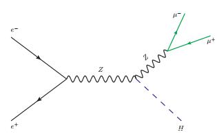Figure1. (color online) LO diagram for e⁺e^?→μ⁺μ^-H.

$\begin{eqnarray}\begin{array}{ll}{\mathop{ {\mathcal M} }\limits^{\sim }}_{0}&=-\frac{{e}^{3}{M}_{Z}}{{s}_{W}{c}_{W}}\bar{v}({k}_{1}){\Gamma }_{Z}^{\mu }u({k}_{2})\frac{{g}_{\mu \nu }}{(s-{M}_{Z}^{2})({s}_{12}-{M}_{Z}^{2})}\\&\times \bar{u}({p}_{1}){\Gamma }_{Z}^{\nu }v({p}_{2}), \end{array}\end{eqnarray}$

(2)

where c_W ≡ cos θ_W, s_W ≡ sin θ_W, with θ_W the Weinberg angle, M_Z represents the mass of the Z⁰ boson. ${\Gamma }_{V}^{\mu }={g}_{V}^{+}{\gamma }^{\mu }\frac{1+{\gamma }^{5}}{2}+{g}_{V}^{-}{\gamma }^{\mu }\frac{1-{\gamma }^{5}}{2}$ is the coupling of the gauge boson and the charged lepton. Specifically speaking, ${g}_{Z}^{+}=\frac{{s}_{W}}{{c}_{W}}$, ${g}_{Z}^{-}=\frac{{s}_{W}}{{c}_{W}}-\frac{1}{2{s}_{W}{c}_{W}}$. The chirality structure of the neutral current demands that, e⁺ and e^? (also μ⁺ and μ^-) must carry opposite helicity in order to render a non-vanishing amplitude.
As can be readily seen from Fig. 1, it is possible for the μ⁺μ^- pair to be resonantly produced from the on-shell Z⁰ boson, consequently the amplitude in (2) blows up at ${s}_{12}={M}_{Z}^{2}$, which reflects that fixed-order calculation breaks down near the Z pole. To tame the singularity in the limit ${s}_{12}\to {M}_{Z}^{2}$, it is customary to replace the second Z boson propagator in (2) with the Breit-Wigner form, which amounts to include the Dyson summation for the Z boson self-energy diagrams. Retaining finite Z width would effectively cutoff the IR singularity. One may define a new amplitude:

$\begin{eqnarray}{ {\mathcal M} }_{0}= {\mathcal F} {\mathop{ {\mathcal M} }\limits^{\sim }}_{0}, {\mathcal F} =\frac{{s}_{12}-{M}_{Z}^{2}}{{s}_{12}-{M}_{Z}^{2}+i{M}_{Z}{\Gamma }_{Z}}, \end{eqnarray}$

(3)

where $ {\mathcal F} $ is a rescaling factor, and Γ_Z signifies the width of the Z⁰ boson.
The LO cross section is then given by

$\begin{eqnarray}{\sigma }_{0}=\frac{1}{2s}\displaystyle \int {\rm{d}}{\Pi }_{3}\frac{1}{4}\displaystyle \sum _{{\rm{Pol}}}{|{ {\mathcal M} }_{0}|}^{2}, \end{eqnarray}$

(4)

where the three-body phase space in the center-of-mass (CM) frame can be conveniently parameterized as

$\begin{eqnarray}\begin{array}{ll}\displaystyle \int {\rm{d}}{\Pi }_{3}&=\displaystyle \int \frac{{{\rm{d}}}^{3}{p}_{1}}{{(2\pi )}^{3}2{p}_{1}^{0}}\frac{{{\rm{d}}}^{3}{p}_{2}}{{(2\pi )}^{3}2{p}_{2}^{0}}\frac{{{\rm{d}}}^{3}{p}_{H}}{{(2\pi )}^{3}2{p}_{H}^{0}}\\&\times {(2\pi )}^{4}{\delta }^{(4)}({k}_{1}+{k}_{2}-{p}_{1}-{p}_{2}-{p}_{H})\\&=\frac{1}{{(2\pi )}^{4}}\frac{1}{16\sqrt{s}}\displaystyle \int \frac{{\rm{d}}{s}_{12}}{\sqrt{{s}_{12}}}{\rm{d}}{\Omega }_{1}^{* }{\rm{d}}\cos {\theta }_{H}|{{\boldsymbol{p}}}_{1}^{* }||{{\boldsymbol{p}}}_{H}|, \end{array}\end{eqnarray}$

(5)

where $(|{{\boldsymbol{p}}}_{1}^{* }|, {\Omega }_{1}^{* })$ signifies the 3-momentum of the μ^- in the rest frame of the dimuon system, |p_H|, θ_H represent the magnitude of the momentum and the polar angle of the Higgs boson in the laboratory frame, respectively. Upon neglecting masses of the electron and muon, one obtains $|{{\boldsymbol{p}}}_{1}^{* }|={M}_{\mu \mu }/2$, and $|{{\boldsymbol{p}}}_{H}|=\frac{1}{2\sqrt{s}}{\lambda }^{1/2}(s, {s}_{12}, {M}_{H}^{2})$, where λ (a, b, c)≡a²+b²+c²?2ab?2ac?2bc is the K?llén function. In deriving (5), we have utilized the axial symmetry to eliminate the trivial dependence on the azimuthal angle of the outgoing Higgs boson.
Squaring (2), summing over μ⁺μ^- helicities, and averaging upon the e⁺e^? polarizations, one observes that the squared amplitude bears a factorized structure, thanks to the simple s-channel topology. Substituting it into (4), integrating over the solid angle ${\Omega }_{1}^{* }$, one then arrives at the following double differential cross section:

$\begin{eqnarray}\begin{array}{ll}\frac{{{\rm{d}}}^{2}{\sigma }_{0}}{{\rm{d}}{s}_{12}{\rm{d}}\cos {\theta }_{H}}=&\frac{{\alpha }^{3}{({g}_{Z}^{+2}+{g}_{Z}^{-2})}^{2}}{24{c}_{W}^{2}{s}_{W}^{2}}\frac{|{{\boldsymbol{p}}}_{H}|{M}_{Z}^{2}}{\sqrt{s}{(s-{M}_{Z}^{2})}^{2}}\\&\times \frac{{s}_{12}}{{({s}_{12}-{M}_{Z}^{2})}^{2}+{M}_{Z}^{2}{\Gamma }_{Z}^{2}}\left(2+{\sin }^{2}\theta \frac{{{\boldsymbol{p}}}_{H}^{2}}{{s}_{12}}\right), \end{array}\end{eqnarray}$

(6)

with $\alpha \equiv \frac{{e}^{2}}{4\pi }$ the electromagnetic fine structure constant.
Integrating (6) over the polar angle, one obtains the Born-order spectrum of the invariant mass of μ⁺μ^-:

$\begin{eqnarray}\begin{array}{ll}\frac{{\rm{d}}{\sigma }_{0}}{{\rm{d}}{M}_{\mu \mu }}&=\frac{{\alpha }^{3}{({g}_{Z}^{+2}+{g}_{Z}^{-2})}^{2}}{9{c}_{W}^{2}{s}_{W}^{2}}\frac{|{{\boldsymbol{p}}}_{H}|{M}_{Z}^{2}}{\sqrt{s}{(s-{m}_{Z}^{2})}^{2}}\\&\times \frac{{s}_{12}^{3/2}}{{({s}_{12}-{M}_{Z}^{2})}^{2}+{M}_{Z}^{2}{\Gamma }_{Z}^{2}}(3+\frac{{{\boldsymbol{p}}}_{H}^{2}}{{s}_{12}}).\end{array}\end{eqnarray}$

(7)

Since Γ_Z?M_Z, one naturally expects that the NWA should be fairly reliable for the process under consideration. Inserting the limiting formula

$\begin{eqnarray}\mathop{\mathrm{lim}}\limits_{{\Gamma }_{Z}\to 0}\frac{1}{{({s}_{12}-{M}_{Z}^{2})}^{2}+{M}_{Z}^{2}{\Gamma }_{Z}^{2}}=\frac{\pi }{{M}_{Z}{\Gamma }_{Z}}\delta ({s}_{12}-{M}_{Z}^{2})\end{eqnarray}$

(8)

into (6), and integrating over s₁₂, we obtain the angular distribution:

$\begin{eqnarray}{\left.\frac{{\rm{d}}{\sigma }_{0}}{{\rm{d}}\cos {\theta }_{H}}\right|}_{{\rm{NWA}}}=\frac{{\rm{d}}{\sigma }_{0}(ZH)}{{\rm{d}}\cos \theta }{{\rm{Br}}}_{0}(Z\to {\mu }^{+}{\mu }^{-}), \end{eqnarray}$

(9)

where

$\begin{eqnarray}\frac{{\rm{d}}{\sigma }_{0}(ZH)}{{\rm{d}}\cos \theta }=\frac{\pi {\alpha }^{2}({g}_{Z}^{+2}+{g}_{Z}^{-2})}{4{c}_{W}^{2}{s}_{W}^{2}}\frac{|{{\boldsymbol{p}}}_{H}|{M}_{Z}^{2}}{\sqrt{s}{(s-{M}_{Z}^{2})}^{2}}\left(2+{\sin }^{2}\theta \frac{{{\boldsymbol{p}}}_{Z}^{2}}{{M}_{Z}^{2}}\right), \end{eqnarray}$

(10)

is the angular distribution of the Z(H) in the process e⁺e^? → ZH at Born order, with $|{{\boldsymbol{p}}}_{H}|\equiv \frac{1}{2\sqrt{s}}{\lambda }^{1/2}(s, {M}_{Z}^{2}, {M}_{H}^{2})$. In (9), the Born-order partial width and branching fraction of Z→μ⁺μ^- are given by

$\begin{eqnarray}{\Gamma }_{0}(Z\to {\mu }^{+}{\mu }^{-})=\frac{\alpha }{6}({g}_{Z}^{+2}+{g}_{Z}^{-2}){M}_{Z}, \end{eqnarray}$

(11a)

$\begin{eqnarray}{{\rm{Br}}}_{0}(Z\to {\mu }^{+}{\mu }^{-})\equiv \frac{{\Gamma }_{0}(Z\to {\mu }^{+}{\mu }^{-})}{{\Gamma }_{Z}}.\end{eqnarray}$

(11b)

From (9), one readily obtains the LO integrated cross section in the NWA ansatz:

$\begin{eqnarray}{\sigma }_{0}({\mu }^{+}{\mu }^{-}H){|}_{{\rm{NWA}}}={\sigma }_{0}(ZH){{\rm{Br}}}_{0}(Z\to {\mu }^{+}{\mu }^{-}), \end{eqnarray}$

(12)

where

$\begin{eqnarray}{\sigma }_{0}(ZH)=\frac{\pi {\alpha }^{2}({g}_{Z}^{+2}+{g}_{Z}^{-2})}{3{c}_{W}^{2}{s}_{W}^{2}}\frac{|{{\boldsymbol{p}}}_{H}|{M}_{Z}^{2}}{\sqrt{s}{(s-{M}_{Z}^{2})}^{2}}\left(3+\frac{{{\boldsymbol{p}}}_{Z}^{2}}{{M}_{Z}^{2}}\right).\end{eqnarray}$

(13)

Note that the unpolarized LO cross section σ₀(ZH) in (13) decreases rather mildly (∝ 1/s) in the high energy limit, reflecting the dominance of producing the longitudinally polarized Z in large $\sqrt{s}$. However, at moderate energy such as $\sqrt{s}=250$ GeV at CEPC, the longitudinally-polarized cross section only comprises of 42% of the total unpolarized cross section.

As mentioned before, in this work we are interested in addressing the NLO weak and mixed electroweak-QCD corrections for e⁺e^?→μ⁺μ^-H:

$\begin{eqnarray} {\mathcal M} ={ {\mathcal M} }_{0}+{ {\mathcal M} }^{(\alpha )}+{ {\mathcal M} }^{(\alpha {\alpha }_{s})}+\cdots .\end{eqnarray}$

(14)

For simplicity, in this work we have neglected the pure QED corrections (such as ISR and FSR effect), which can instead be simulated by the package Whizard [30]. As a consequence, a simplifying feature arises that the dominant higher-order diagrams resemble the s-channel topology as depicted in Fig. 1, which contains only one resonant Z propagator.
Once going beyond LO, it becomes a quite delicate issue to incorporate the finite Z width effect yet without spoiling gauge invariance and bringing double counting. Over the past decades, numerous practical schemes have been proposed to tackle the unstable particle, such as the pole scheme [31-33], factorization scheme [34, 35], fermion-loop scheme [36, 37], boson-loop scheme [38], complex mass scheme [39, 40], etc.. It is worth mentioning that a systematic and model-independent approach, the unstable particle effective theory, has also emerged finally [41, 42]. However, this approach is valid only near the resonance peak, and cannot be applied in the entire kinematic range.
Owing to the particularly simple s-channel topology of our process, it is most convenient to employ the factorization scheme [34, 35], which is particularly suitable for such resonance-dominated process. In this scheme, one rescales a gauge-invariant higher-order amplitude by a Breit-Wigner factor $ {\mathcal F} $, and subtracting the iM_ZΓ_Z terms which potentially generates double counting. The merit of this scheme is that gauge invariance is preserved, and can be readily implemented in automated calculation. Recently this scheme has also been used by Denner et al. to analyze the NLO electroweak correction to ${e}^{+}{e}^{-}\to \nu \bar{\nu }H$ [25].
For our purpose, we specify the recipe of the factorization scheme closely following [25]:

$\begin{eqnarray}{ {\mathcal M} }^{(\alpha {\alpha }_{s}^{n})}= {\mathcal F} {\mathop{ {\mathcal M} }\limits^{\sim }}^{(\alpha {\alpha }_{s}^{n})}+i\frac{{\rm{Im}}\{{\hat{\Sigma }}_{T}^{ZZ\, (\alpha {\alpha }_{s}^{n})}({M}_{Z}^{2})\}}{{s}_{12}-{M}_{Z}^{2}}{ {\mathcal M} }_{0}, \end{eqnarray}$

(15)

where n=0, 1, $\mathop{M}\limits^{\sim }$ represents the fixed-order amplitude where the Z⁰ is treated as a rigorously stable particle, $ {\mathcal F} $ and ${ {\mathcal M} }_{0}$ have been defined in (3), ${\hat{\Sigma }}_{ZZ}^{T}(s)$ represents the transverse part of the renormalized one-particle irreducible self-energy diagrams for Z boson. M_Z is the pole mass of the Z⁰ boson, and throughout the work we take Γ_Z as the experimentally determined Z⁰ boson width¹⁾.
1) By default, the pole mass of the Z⁰ is determined by the condition ${\rm{Re}}\{{\hat{\Sigma }}_{ZZ}({M}_{Z}^{2})\}\equiv 0$, whereas its width is inferred from the optical theorem, ${M}_{Z}{\Gamma }_{Z}={\rm{Im}}\{{\hat{\Sigma }}_{ZZ}({M}_{Z}^{2})\}$. It was argued [32, 33, 43] that the pole mass and the corresponding width defined this way are gauge dependent. Nevertheless, the gauge-dependent terms arise at order-α³ in the’t Hooft-Feynman gauge, which is beyond the accuracy targeted in this work. Thus we will pretend M_Z and Γ_Z to be gauge-invariant quantities.
The second term in the right-hand side of (15) is included to subtract the double-counting term. Fortunately, due to its orthogonal phase, the interference of this term with $\mathop{ {\mathcal M} }\limits^{\sim }$ generates a purely imaginary contribution to the cross section, thus can be safely neglected.
Once the rescaled ${\mathcal{O}}(\alpha )$ and ${\mathcal{O}}(\alpha {\alpha }_{s})$ amplitudes are obtained, we then deduce the corresponding higher-order corrections to the differential cross section through

$\begin{eqnarray}{\sigma }^{(\alpha {\alpha }_{s}^{n})}=\frac{1}{2s}\displaystyle \int {\rm{d}}{\Pi }_{3}\frac{1}{4}\displaystyle \sum _{{\rm{Pol}}}2{\rm{Re}}[{ {\mathcal M} }_{0}^{* }{ {\mathcal M} }^{(\alpha {\alpha }_{s}^{n})}], \end{eqnarray}$

(16)

with n=0, 1. Note even for the mixed electroweak-QCD correction, we only need consider its interference with the Born-order amplitude.
We conclude this section by stressing that, since the non-resonant diagrams are regular at ${s}_{12}={M}_{Z}^{2}$, the rescaling procedure in (15) enforces their contributions to the amplitude to vanish on the Z⁰ pole. In the vicinity of the resonance, it is intuitively appealing that the non-resonant diagrams are much more suppressed relative to the resonant diagrams. As will be seen in Section 6, our numerical predictions indeed confirm this anticipation.

We now outline the calculation of the NLO weak correction to e⁺e^?→μ⁺μ^-H, with some representative diagrams depicted in Fig. 2 and 3. As stressed before, we will not consider the ISR and FSR types of diagrams. It is obvious that the NLO diagrams can be separated into two gauge-invariant subgroups, with either “resonant” or “non-resonant” structures. For the former subset, the diagrams are very similar to those encountered in the previous NLO weak correction for e⁺e^? → ZH, so are the corresponding calculations; for the latter, there emerges no singularity as ${s}_{12}\to {M}_{Z}^{2}$, so there is no need to include width effect for any particle routing around the loop.
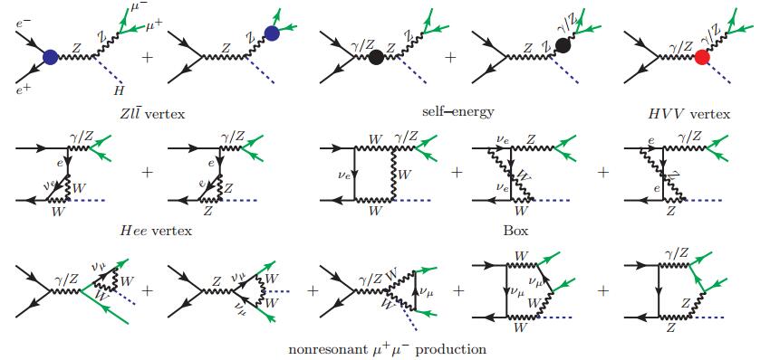Figure2. (color online) Some representative higher-order diagrams for e⁺e^?→μ⁺μ^-H, through the order-αα_s. The three solidheavy dots are explained in Fig. 3. Diagrams in the first two rows correspond to the “resonant” channel e⁺e^?→(Z^*/γ^*→)μ⁺μ^-+H, while those in the last row exhibit a completely different “non-resonant” topology.

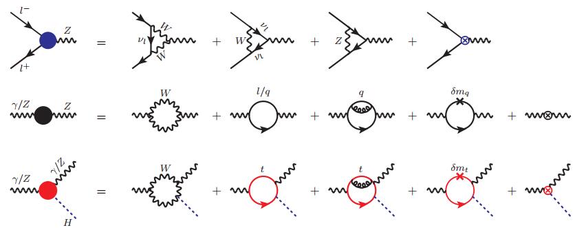Figure3. (color online) Representative diagrams for the radiative corrections to the renormalized Zee vertex, γ/Z self-energy, and HVV vertex, through order-αα_s. The cross represents the quark mass counterterm in QCD, cap denotes the electroweak counterterm in on-shell scheme.

The NLO amplitude is computed in Feynman gauge. Masses of all light fermions are neglected except the top quark. Dimensional regularization (DR) is employed to regularize UV divergence. The Feynman diagrams and the corresponding amplitude are generated by the package FeynArts [44]. Tensor contraction and Dirac/color matrices trace are conducted by using FeynCalc and FeynCalcFormLink [45-47]. Tensor integrals are further reduced to the Passarino-Veltman scalar functions, which are numerically evaluated by Collier [48] and LoopTools [49].
We also choose to use the standard on-shell renormalization scheme to sweep UV divergences, where various electroweak counterterms are tabulated in [50]. Depending on the specific recipe for the charge renormalization constant Z_e, there are three popular sub-schemes of the on-shell renormalization: α(0), α(M_Z) and G_μ schemes [13]. In the first scheme, the fine structure constant α is assuming its Thomson-limit value, whereas α(0) is replaced with

$\begin{eqnarray}\alpha ({M}_{Z})\, =\frac{\alpha (0)}{1-\Delta \alpha ({M}_{Z})}, \end{eqnarray}$

(17a)

$\begin{eqnarray}{\alpha }_{{G}_{\mu }}\, =\frac{\sqrt{2}}{\pi }{G}_{\mu }{M}_{W}^{2}{s}_{W}^{2}, \end{eqnarray}$

(17b)

in the α(M_Z) and G_μ schemes, respectively. Differing from the α(0) scheme, these two schemes effectively resum either some universal large logarithms from the light fermion loop or some ${m}_{t}^{2}$-enhanced terms from the top quark loop.
Once the ${\mathop{ {\mathcal M} }\limits^{\sim }}^{(\alpha )}$ is rendered finite after the renormalization procedure, we then employ (15) to obtain the rescaled amplitude ${ {\mathcal M} }^{(\alpha )}$, which encapsulates the finite Z-width effect. It is then straightforward to utilize (16) to infer the NLO weak correction to the differential cross section.

Finally we turn to the ${\mathcal{O}}(\alpha {\alpha }_{s})$ mixed electroweak-QCD correction to e⁺e^?→μ⁺μ^-H. Since it is the quarks instead of leptons that can experience the strong color force, we only need retain those diagrams involving quark loop. Moreover, since the top quark couples the Higgs boson with the strongest strength, for simplicity we have neglected the masses of all lighter quarks, so we only retain those two-loop diagrams where only the top quark loop dressed by gluon. Some typical two-loop diagrams are shown in Fig. 2 and 3, bearing only the s-channel “resonant” structure. As indicated in Fig. 3, at this order, QCD renormalization is realized by merely inserting the one-loop top quark mass counterterm, δm_t, into the internal top-quark propagator, as well as into the $Ht\bar{t}$ vertex [15]. The calculation very much resembles our preceding work on ${\mathcal{O}}(\alpha {\alpha }_{s})$ correction to e⁺e^? → ZH [15], and we referred the interested readers to that paper for more details.
For the actual two-loop computation, we utilize the packages Apart [51] and FIRE [52] to perform partial fraction and integration-by-parts (IBP) reduction. We then combine FIESTA [53]/CubPack [54] to perform sector decomposition and subsequent numerical integrations for master integrals with quadruple precision.
Besides the finite renormalization of Zee vertex [15], the ${\mathcal{O}}(\alpha {\alpha }_{s})$ amplitude can be expressed in terms of the Born-order amplitude supplemented with an effective HVV vertex:

$\begin{eqnarray}\begin{array}{ll}{\mathop{ {\mathcal M} }\limits^{\sim }}^{(\alpha {\alpha }_{s})}&=\displaystyle \sum _{{V}_{1}, {V}_{2}=Z, \gamma }\frac{-{e}^{2}}{{s}^{2}-{M}_{{V}_{1}}^{2}}\bar{v}({k}_{1}){\Gamma }_{{V}_{1}, \mu }u({k}_{2})\bar{u}({p}_{1})\\&\times {\Gamma }_{{V}_{2}, \nu }v({p}_{2})\frac{1}{{s}_{12}-{M}_{{V}_{2}}^{2}}(-ie){T}_{{V}_{1}{V}_{2}H}^{\mu \nu }(K, P), \end{array}\end{eqnarray}$

(18)

where the sum is extended over V₁, V₂ = Z⁰, γ, and $-ie{T}_{H{V}_{1}{V}_{2}}^{\mu \nu }$ is the HV₁V₂ effective vertex, which depends on K = k₁+k₂ and P = p₁+p₂. The gauge boson V₁ is coupled with the incoming e⁺e^? pair, whereas the gauge boson V₂ is affiliated with the outgoing μ⁺μ^- pair. ${\Gamma }_{V}^{\mu }$ represents the coupling between the gauge boson and charged leptons, whose form has already been specified in the paragraph after (2). The electromagnetic coupling of lepton is chiral symmetric, ${g}_{\gamma }^{\pm }=1$.
By Lorentz covariance, the renormalized vertex tensor ${T}_{H{V}_{1}{V}_{2}}^{\mu \nu }$ can be decomposed as

$\begin{eqnarray}\begin{array}{ll}{T}_{H{V}_{1}{V}_{2}}^{\mu \nu }&={T}_{1}\frac{{K}^{\mu }{K}^{\nu }}{s}+{T}_{2}{P}^{\mu }{P}^{\nu }+{T}_{3}\frac{{K}^{\mu }{P}^{\nu }}{s}+{T}_{4}\frac{{P}^{\mu }{K}^{\nu }}{s}\\&+{T}_{5}{g}^{\mu \nu }+{T}_{6}{\epsilon }^{\mu \nu \alpha \beta }\frac{{K}^{\alpha }{P}^{\beta }}{s}, \end{array}\end{eqnarray}$

(19)

where T_i(i=1, ? , 6) are Lorentz scalar solely depending on s, s₁₂ and ${M}_{{V}_{1, 2}}^{2}$. Furry theorem enforces that T₆=0, technically because C-invariance forbids a single γ⁵ to emerge in the trace over the fermionic loop. Owing to the current conservation associated with massless leptons, it turns out that only the scalar form factors T_{4, 5} survive in the differential cross sections.
Substituting (19) into (18), utilizing the factorization scheme (15) to implement the finite Z⁰ width effect, we then obtain the rescaled amplitude ${ {\mathcal M} }^{(\alpha {\alpha }_{s})}$. From (16), we find the ${\mathcal{O}}(\alpha {\alpha }_{s})$ mixed electroweak-QCD correction to the differential cross section to be

$\begin{eqnarray}\begin{array}{ll}\frac{{\rm{d}}{\sigma }^{(\alpha {\alpha }_{s})}}{{\rm{d}}{s}_{12}}&=\frac{{\alpha }^{3}{M}_{Z}}{9{c}_{W}{s}_{W}\sqrt{s}}{| {\mathcal F} |}^{2}\\&\times \displaystyle \sum _{{V}_{1}, {V}_{2}=Z, \gamma }\frac{({g}_{{V}_{1}}^{-}{g}_{Z}^{-}+{g}_{{V}_{1}}^{+}{g}_{Z}^{+})({g}_{{V}_{2}}^{-}{g}_{Z}^{-}+{g}_{{V}_{2}}^{+}{g}_{Z}^{+})}{(s-{M}_{Z}^{2})(s-{M}_{{V}_{1}}^{2})}\\&\times \frac{{s}_{12}|{{\boldsymbol{p}}}_{H}|}{({s}_{12}-{M}_{Z}^{2})({s}_{12}-{M}_{{V}_{2}}^{2})}{{\mathcal{T}}}_{{V}_{1}{V}_{2}}, \end{array}\end{eqnarray}$

(20)

where

$\begin{eqnarray}{{\mathcal{T}}}_{{V}_{1}{V}_{2}}=\frac{{{\boldsymbol{p}}}_{H}^{2}}{2}\left(\frac{1}{{s}_{12}}-\frac{{M}_{H}^{2}}{{s}_{12}s}+\frac{1}{s}\right){T}_{4}+\left(\frac{{{\boldsymbol{p}}}_{H}^{2}}{{s}_{12}}+3\right){T}_{5}.\end{eqnarray}$

(21)

Following [15], we take $\sqrt{s}=240$, 250 GeV as two benchmark CM energies at CEPC. We adopt the following values for the input parameters [22]: M_H = 125.09 GeV, M_Z = 91.1876(21) GeV, Γ_Z = 2.4952(23) GeV, M_W = 80.385(15) GeV, m_t = 174.2± 1.4 GeV, G_μ = 1.166 3787(6)×10^?5GeV^?2, α(0) = 1/137.035999, $\Delta {\alpha }_{{\rm{had}}}^{(5)}=0.02764(13)$, and α(M_Z) = 1/128.943 in the α(M_Z) scheme. To analyze the mixed electroweak-QCD correction, we take α_s(M_Z)=0.1185, and use the package RunDec [55] to evaluate the QCD running coupling constant at other scales.
The angular distribution of Higgs boson at $\sqrt{s}=240$ GeV is depicted in Fig. 4, including both NLO weak and mixed electroweak-QCD corrections. We stay with the α(0) scheme, and fix $\mu =\sqrt{s}/2$ for the QCD coupling, and take ${\alpha }_{s}(\sqrt{s}/2)=0.1135$. The impact of the ${\mathcal{O}}(\alpha )$ and ${\mathcal{O}}(\alpha {\alpha }_{s})$ corrections to the Higgs angular distribution is quite analogous to what is found in our preceding work on e⁺e^?→ZH [15]. In Fig. 5, we also show the μ⁺μ^- invariant mass spectrum at $\sqrt{s}=240$ GeV, including both NLO weak and mixed electroweak-QCD corrections. As expected, the spectrum develops a sharp Breit-Wigner peak around the Z resonance. The ${\mathcal{O}}(\alpha )$ and ${\mathcal{O}}(\alpha {\alpha }_{s})$ corrections play a very minor role except in the proximity of the Z pole. It is interesting for the future measurement of the di-muon spectrum at CEPC to examine our predictions.
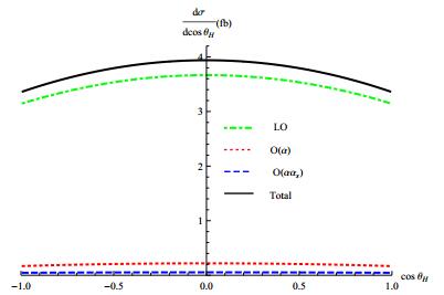Figure4. (color online) Angular distribution of the Higgs boson at $\sqrt{s}=240$ GeV, shown at various levels of perturbative accuracy.

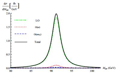Figure5. (color online) μ⁺μ^- invariant mass spectrum at $\sqrt{s}=240$ GeV, at various levels of perturbative accuracy.

In Table 1, we supplement more details for the dimuon invariant mass spectrum. We divide the NLO weak correction into the contribution from the resonant diagrams and the one from non-resonant diagrams. As can be seen from the Table 1, the ${\mathcal{O}}(\alpha )$ correction is saturated by the resonant diagrams almost in the entire energy range, especially near the Z peak.

		50	70	80	85	90	91	92	95	100	110	σ
LO/fb		0.66	2.39	8.03	24.45	309.02	570.98	407.45	53.27	9.66	1.31	6.9828
${\mathcal{O}}(\alpha )$	resonant/fb	0.04	0.14	0.47	1.42	17.78	32.82	23.39	3.05	0.55	0.07	0.4015
	nonresonant (10?4/fb)	65	39	22	12	1	0	-0	-7	-16	-24	8.5
${\mathcal{O}}(\alpha {\alpha }_{s})$/fb		0.01	0.04	0.13	0.35	4.54	8.37	5.97	0.79	0.15	0.02	0.103

Table1.Differential cross section with respect to the μ⁺μ^- invariant mass at $\sqrt{s}=240$ GeV. Note the upper bound for M_{μ μ} equals $\sqrt{s}-{M}_{H}$.

Our goal is to present to date the most comprehensive predictions for the e⁺e^? → μ⁺μ^-H process, taking into various sorts of theoretical uncertainties account. In Table 2, we present our LO, NLO, NNLO predictions for the integrated cross section at $\sqrt{s}=240(250)$ GeV. The results are provided with three renormalization sub-schemes. We also include the uncertainty inherent in the input parameters (first error) and the uncertainty due to the QCD renormalization scale (second error). To assess the parametric uncertainty, we vary the values of M_W and m_t, and $\Delta {\alpha }_{{\rm{had}}}^{(5)}$ around the central PDG values within the 1σ bands. For the QCD scale uncertainty, we slide the μ in α_s from M_Z to $\sqrt{s}$.

$\sqrt{s}$/GeV	schemes	σLO/fb	σNLO/fb	σNNLO/fb
240	α(0)	${6.983}_{-0.023}^{+0.023}$	${7.385}_{-0.037}^{+0.037}$	${7.488}_{-0.036-0.009}^{+0.036+0.004}$
	α(MZ)	${8.382}_{-0.027}^{+0.028}$	${7.317}_{-0.036}^{+0.037}$	${7.448}_{-0.035-0.011}^{+0.036+0.005}$
	Gμ	${7.772}_{-0.004}^{+0.004}$	${7.527}_{-0.017}^{+0.016}$	${7.554}_{-0.017-0.002}^{+0.017+0.001}$
250	α(0)	${7.036}_{-0.023}^{+0.023}$	${7.424}_{-0.037}^{+0.037}$	${7.527}_{-0.037-0.009}^{+0.037+0.005}$
	α(MZ)	${8.446}_{-0.028}^{+0.028}$	${7.350}_{-0.036}^{+0.037}$	${7.481}_{-0.037-0.011}^{+0.037+0.006}$
	Gμ	${7.831}_{-0.004}^{+0.004}$	${7.564}_{-0.017}^{+0.017}$	${7.591}_{-0.016-0.002}^{+0.017+0.001}$

Table2.The total cross section for e⁺e^?→μ⁺μ^-H at $\sqrt{s}=240(250)$ GeV. The LO, NLO, and NNLO predecitions are presented with three renormalization sub-schemes. To estimate the parametric uncertainty, we take M_W = 80.385±0.015 GeV, m_t=174.2±1.4 GeV, and $\Delta {\alpha }_{{\rm{had}}}^{(5)}=0.02764\pm 0.00013$. We also vary the QCD coupling constant from α_s(M_Z) to ${\alpha }_{s}(\sqrt{s})$, with the central value taken as ${\alpha }_{s}(\sqrt{s}/2)$.

From Table 2, we observe a very similar pattern of scheme and parametric dependence of higher-order corrections as [15]. While the parametric and scale uncertainties of the NNLO predictions in the α(0) and α(M_Z) schemes are both about 0.5% of the NNLO results, the relative errors are somewhat reduced in the G_μ scheme (≈0.2%). We also find that in the G_μ scheme, the mixed electroweak-QCD corrections only amount to 0.4% of LO cross section, which might be attributed to the fact that in addition to the running of α, universal corrections to the ρ parameter are also absorbed into the LO cross section. As can also be seen in Table 2, though the predicted LO cross sections from three renormalization schemes differ significantly, including the NLO weak correction significantly help them converge to each other. Including mixed electroweak-QCD correction appears not to further reduce the scheme dependence. To yield a scheme-insensitive prediction, it appears to be imperative to continue to compute the NNLO electroweak correction, which is certainly an extremely daunting task.
Since Γ_Z?M_Z, and the production rate is predominantly saturated by the Z⁰ resonance. It may seem natural to anticipate that the NWA remains valid even after including higher order corrections. Under the assumption of NWA, one may approximate the LO cross section and the higher-order radiative corrections by

$\begin{eqnarray}{\sigma }_{0}{|}_{{\rm{NWA}}}={\sigma }_{0}(ZH){{\rm{Br}}}_{0}(Z\to {\mu }^{+}{\mu }^{-}), \end{eqnarray}$

(22a)

$\begin{eqnarray}\begin{array}{ll}{\sigma }^{(\alpha )}{|}_{{\rm{NWA}}}&={\sigma }^{(\alpha )}(ZH){{\rm{Br}}}_{0}(Z\to {\mu }^{+}{\mu }^{-})\\&+{\sigma }_{0}(ZH){{\rm{Br}}}^{(\alpha )}(Z\to {\mu }^{+}{\mu }^{-}), \end{array}\end{eqnarray}$

(22b)

$\begin{eqnarray}\begin{array}{ll}{\sigma }^{(\alpha {\alpha }_{s})}{|}_{{\rm{NWA}}}&={\sigma }^{(\alpha {\alpha }_{s})}(ZH){{\rm{Br}}}_{0}(Z\to {\mu }^{+}{\mu }^{-})\\&+{\sigma }_{0}(ZH){{\rm{Br}}}^{(\alpha {\alpha }_{s})}(Z\to {\mu }^{+}{\mu }^{-}), \end{array}\end{eqnarray}$

(22c)

where σ(ZH) represents the Higgsstrahlung cross section, with σ₀(ZH) given in (13). Br₀ is defined in (11), and the radiative corrections ${{\rm{Br}}}^{(\alpha {\alpha }_{s}^{n})}$ (n = 0, 1) can be read off from

$\begin{eqnarray}\begin{array}{ll}{\rm{Br}}(Z\to {\mu }^{+}{\mu }^{-})=&{{\rm{Br}}}_{0}(Z\to {\mu }^{+}{\mu }^{-})+{{\rm{Br}}}^{(\alpha )}(Z\to {\mu }^{+}{\mu }^{-})\\&+{{\rm{Br}}}^{(\alpha {\alpha }_{s})}(Z\to {\mu }^{+}{\mu }^{-})+\cdots .\end{array}\end{eqnarray}$

(23)

Since the width of the Z⁰ is held fixed, the perturbative expansion for the branching fraction of Z⁰→μ⁺μ^- amounts to the expansion for the corresponding partial width.
In Table 3, we compare the predicted e⁺e^?→μ⁺μ^-H cross section from the literal full calculation with that from NWA. For the sake of concreteness, we take $\sqrt{s}=240$ GeV, and employ the α(0) scheme. At LO, the NWA prediction is about 3% higher than the full prediction, while ${\mathcal{O}}(\alpha )$ and ${\mathcal{O}}(\alpha {\alpha }_{s})$ corrections are observed to be only slightly different. As a consequence, the NWA prediction to the total cross section at NNLO accuracy turns out to be about 4% higher than the full NNLO prediction.

	LO	NLO	NNLO
σ/fb	6.983	7.385	7.488
σ|NWA/fb	7.241	7.657	7.760

Table3.Compare the full and NWA predictions to the cross sections at $\sqrt{s}=240$ GeV, at various levels of perturbative accuracy.

Higgsstrahlung is the leading Higgs production mechanism at CEPC. The mixed electroweak-QCD correction to e⁺e^? → ZH has recently become available [14, 15]. This piece of NNLO correction appears to be surprisingly large, about 1% of the Born-order result, therefore must be considered when matching the exquisite experimental accuracy.
To make closer contact with the actual experimental measurement, in this work we have investigated both NLO weak and mixed electroweak-QCD corrections to one of the golden mode in CEPC, i.e. e⁺e^?→μ⁺μ^-H, with the finite Z⁰ width properly accounted. At $\sqrt{s}\approx 240$ GeV, the NLO weak correction may reach 6% of the Born order cross section, while the NNLO mixed electroweak-QCD correction can reach 1.5% of the LO cross section, greater than the projected experimental accuracy of 0.9%. We also present numerical predictions to various differential cross sections at NNLO accuracy, in particular we predict the μ⁺μ^- invariant-mass spectrum of the Breit-Wigner shape. We have also compared our full predictions with those based on the NWA, and found the agreement within a few percents. It is interesting to await the future experiment to examine our predictions.
We also carefully address the issue about scheme-dependence of our predictions, at various levels of perturbative accuracy. Employing three popular renormalization sub-schemes, we find that the predicted LO cross sections substantially differ from each other. Including the NLO weak correction is crucial to stabilize the predictions from different schemes, however including mixed electroweak-QCD correction seems not to help. To yield a scheme-insensitive prediction, it appears to be compulsory to continue to include the NNLO electroweak correction.
We are grateful to Gang Li and Qing-Feng Sun for useful discussions.