苟斐斐^1,2, 刘建军³, 刘卫东², 罗莉涛^1,2
1. 中国科学院大学, 北京 100049;
2. 中国科学院渗流流体力学研究所, 河北 廊坊 065007;
3. 西南石油大学, 成都 610550
摘要: 研究一类典型的伏尔泰拉积分方程的数值求解方法.通过数值差分离散积分方程,然后将积分方程演化为非线性代数方程组,通过迭代推进求解此类积分方程.分析这种求解方法的代数精度,证明此数值解法的精度高达Δt²阶,可以满足工程计算需要.通过数值仿真验证,数值解与解析解的误差为10^-5.如果采用更高阶的数值积分离散方式,可以获得更高阶精度.
关键词: 伏尔泰拉积分方程非线性数值差分方法误差分析
The Volterra integral equation of the second kind is a special type of integral equations and is often evolved in many engineering domains such as petrol industry. Many methods have been established for solving this kind of equation. Yusufoglu^[1-2] solved systems of the integral equations using the homotopy perturbation and the Lagrange method. Huang et al.^[3] used the Taylor expansion method and obtained an approximate solution. Yang^[4] used the Chebyshev polynomials method to solve the equation,while Yousefi^[5] presented a numerical method for the Abel integral equation by Legendre wavelets. Khodabin et al.^[6] numerically gained the solution of the stochastic Volterra integral equations using triangular functions and their operational matrix of integration. Kamyad et al.^[7] proposed an algorithm based on the calculus of variations and discretization method to solve linear and nonlinear Volterra integral equations. The domain de-composition ^[8-10] was proposed for obtaining the approximate analytic solution of the integral equation.
The integral equation involved in this paper stems from the description of pressure distribution in oil and gas development,and it is given in Eq.(1),

$u\left( t \right)=g\left( t \right)+\int\limits_{0}^{t}{K\left( t-\tau \right)}F\left[ u\left( \tau \right) \right]d\tau ,$

(1)

where the source function g(t) is given and the kernel function K(t) and function F(u) are known to be continuous functions. Function u(t) needs to be determined.
Since the function g(t) is not necessarily zero,this kind of integral equations are generally regarded as non-homogeneous equations. In addition,the transformation of the unknown function by F-function increases the nonlinear degree of the problem. The difficulty in solving this kind of equation numerically is to discrete the integral upper limit and the integral expression synchronously.
1 Discretization of the integral equationIt is obvious in Eq.(1) that,when t=0，u(0) is equal to zero. Based on this fact,a method is proposed by converting the original equation into ordinary differential equation with initial value by derivation and then solving the differential equation. The derivation of the original equation is expressed in Eq.(2),

$\frac{du}{dt}=\frac{dg}{dt}+\frac{d}{dt}\int\limits_{0}^{t}{K\left( t-\tau \right)}F\left[ u\left( \tau \right) \right]d\tau .$

(2)

Practice shows that there is no explicit derivation for this kind of equation,in which convolution is invo-lved. So,the way to the solution goes as following.
If we define that t_i=iΔt (i=0,1,2,…,N) and f(t_i)=f(iΔt)=f_i， we can express the discretization of Eq.(1) in Eq.(4)

$u\left( t \right)=g\left( t \right)+\int\limits_{0}^{t}{K\left( t-\tau \right)}F\left[ u\left( \tau \right) \right]d\tau ,$

(3)

${{u}_{i}}={{g}_{i}}+\int\limits_{0}^{t}{K\left( {{t}_{i}}-\tau \right)}F\left[ u\left( \tau \right) \right]d\tau .$

(4)

And then new designation is defined as

${{\varphi }^{i}}\left( \tau \right)=K\left( {{t}_{i}}-\tau \right)F\left[ u\left( \tau \right) \right],$

(5)

${{Q}_{i}}=\int\limits_{0}^{{{t}_{i}}}{{{\varphi }^{i}}\left( \tau \right)}d\tau ,$

(6)

$u\left( {{t}_{i}} \right)=g\left( {{t}_{i}} \right)+Q\left( {{t}_{i}} \right)$

(7)

where Q_i can be expanded with composite integral formula. Different expansion approaches can be used to get the desirable accuracy. In this paper,composite trapezoidal formula is used. So,Q_i can be expanded as following

$\begin{align} &{{Q}_{i}}\approx \Delta t\sum\limits_{k=0}^{i-1}{\frac{{{\varphi }^{i}}\left( {{t}_{k}} \right)+{{\varphi }^{i}}\left( {{t}_{k+1}} \right)}{2}} \\ &=\Delta t\left( \frac{{{\varphi }^{i}}\left( {{t}_{0}} \right)+{{\varphi }^{i}}\left( {{t}_{i}} \right)}{2}+\sum\limits_{k=0}^{i-1}{{{\varphi }^{i}}\left( {{t}_{k}} \right)} \right). \\ \end{align}$

(8)

Defining

$\varphi _{k}^{i}={{\varphi }^{i}}\left( {{t}_{k}} \right)=K\left( {{t}_{i}}-{{t}_{k}} \right)F\left[ {{u}_{k}} \right]$

(9)

and substituting Eq.(8) into Eq.(7),we get

${{u}_{i}}={{g}_{i}}+{{Q}_{i}}={{g}_{i}}+\Delta t\left( \frac{\varphi _{0}^{i}+\varphi _{i}^{i}}{2}+\sum\limits_{k=1}^{i-1}{\varphi _{k}^{i}} \right).$

(10)

Defining

${{P}_{i}}={{u}_{i}}-\Delta t\frac{\varphi _{i}^{i}}{2}={{u}_{i}}-\Delta t\frac{F\left( 0 \right)F\left( {{u}_{i}} \right)}{2}$

(11)

and substituting Eq.(10) into Eq.(11),we get

${{P}_{i}}={{g}_{i}}+\Delta t\left( \frac{F\left( {{t}_{i}} \right)F\left( {{u}_{0}} \right)}{2}+\sum\limits_{k=1}^{i-1}{K\left( {{t}_{i}}-{{t}_{k}} \right)F\left[ {{u}_{k}} \right]} \right)$

(12)

Since g-function and k-function are known,we can determine the value of P_i using Eq.(12) if new designation U_i-1=[u₀,u₁,…,u_i-1] is known. Then we substitute the known P_i into Eq.(11) to solve the value of u_i.
2 Algorithm and convergence analysisBased on the discretization mentioned above,the specific iteration procedure is as following.
When i=0， then,Q₀=0，u₀=g₀.
When i=1， according to Eq.(10),we have

${{P}_{1}}={{g}_{1}}+\Delta t\frac{K\left( {{t}_{1}} \right)F\left( {{u}_{0}} \right)}{2}$

(13)

Introducing P₁ into Eq.(13),the value of u₁ can be obtained by using the following equation:

${{P}_{1}}={{u}_{1}}-\Delta t\frac{K\left( 0 \right)F\left( {{u}_{1}} \right)}{2}$

(14)

When i=2， by introducing U₁=[u₀,u₁] into Eq.(12),we obtain

${{P}_{2}}={{g}_{2}}+\Delta t\left( \frac{K\left( {{t}_{2}} \right)F\left( {{u}_{0}} \right)}{2}+K\left( {{t}_{2}}-{{t}_{1}} \right)F\left[ {{u}_{1}} \right] \right).$

(15)

And then substituting P₂ into Eq.(11),we get

${{P}_{2}}={{u}_{2}}-\Delta t\frac{K\left( 0 \right)F\left( {{u}_{2}} \right)}{2}.$

(16)

Solving the above equation,we get the value of u₂， which means that U₂=[u₀,u₁,u₂] is available.
When i=n， substituting U_n-1=[u₀,u₁,…,u_n-1] into Eq.(12),we obtain

$\begin{align} &{{P}_{n}}={{g}_{n}}+\Delta t \\ &\left( \frac{K\left( {{t}_{n}} \right)F\left( {{u}_{0}} \right)}{2}+\sum\limits_{k=0}^{i-1}{K\left( {{t}_{n}}-{{t}_{k}} \right)}F\left[ {{u}_{k}} \right] \right) \\ \end{align}$

(17)

Then we get the following equation by introducing P_n into Eq.(11),and we get the expression of P_n,

${{P}_{n}}={{u}_{n}}-\Delta t\frac{K\left( 0 \right)F\left( {{u}_{n}} \right)}{2}.$

(18)

Solving the above equation,we get the value of u_n， which means that U_n=[u₀,u₁,u₂,…,u_n] is available.
The error in this numerical solution rises from the numerical integration in Eq.(8) and the accumulation of error in Eq.(12). The kernel function and F-function are continuous in the solving interval [a,b]. If the second-order derivatives of φ(x) are continuous in the same interval,we can express the truncation error of composite trapezoidal formula in Eq.(9):

${{R}_{N}}\left( \varphi \right)=-\frac{b-a}{12}\Delta {{t}^{2}}\varphi ''\left( \varepsilon \right),a<\varepsilon <b$

(19)

For the above equation,it is obvious that the error has the order of Δt².
It is proved that the accumulation of error is decided by the F-function as follows:
Define the error of u at step N as e_N， and Pe(t_N) as the error of P at the same step. We have

${{e}_{N}}=u\left( {{t}_{N}} \right)-\left( {{u}_{N}} \right)={{e}_{N}}\left( {{R}_{N}}\left( \varphi \right) \right).$

(20)

According to Eq.(12),Pe(t_N) can be expressed as follows:

${{P}_{e}}\left( {{t}_{N}} \right)=\Delta t\sum\limits_{k=1}^{N-1}{K\left( {{t}_{N}}-{{t}_{k}} \right)}F\left[ {{e}_{k}} \right].$

(21)

Since the kernel function and F-function are continuous in interval [a,b]， it is reasonable to assuming that (t_N-t_k)F[e_N]<PR_N. Assuming that the error increases,We have

$P{{e}_{N}}<\Delta t\left( N-1 \right)P{{R}_{N-1}}<\left( b-a \right)P{{R}_{N-1}}.$

(22)

According to Eq.(11),we have

${{e}_{N+1}}=F\left( P{{e}_{N}} \right)<F\left[ \left( b-a \right)P{{R}_{N-1}} \right].$

(23)

In the case that F-function is desirable,the following relationship can be met,

${{e}_{N+1}}<{{e}_{N}}$

(24)

So,the convergence of the problem relies on property of F-function.
3 Case studiesCase 1
To verify the feasibility and accuracy of the proposed method,case studies are given. The related known functions are listed as follows:

$u\left( t \right)=-\frac{1}{2}+\frac{1}{2}{{e}^{2x}}+\int\limits_{0}^{t}{-}{{e}^{2\left( -\tau \right)}}u{{\left( \tau \right)}^{2}}d\tau ,$

(25)

$K\left( x \right)=-{{e}^{2x}},$

(26)

$g\left( x \right)=-\frac{1}{2}+\frac{1}{2}{{e}^{2x}},$

(27)

$F\left( u \right)={{u}^{2}}$

(28)

It is known that the numerical solution of this particular problem is:

$u\left( t \right)=-1+\sqrt{2}\tanh \left( \sqrt{2t}+\frac{1}{2}\log \frac{\sqrt{2}-1}{\sqrt{2}+1} \right).$

(29)

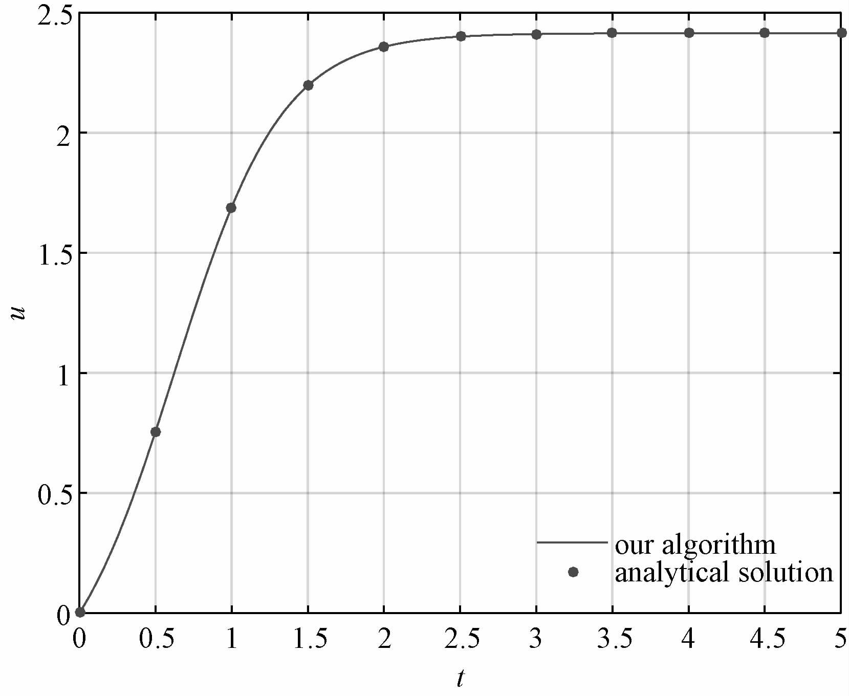
Figure 1 shows the difference between the numerical solution and the analytical solution. The red line indicates the solution of our algorithm and the blue points stand for the analytical solution. In the numerical solution,Δt=0.01 is applied,which means that the solution has an accuracy of 4th order.
Fig. 1

	Download: JPG larger image
Fig. 1 Difference between the numerical solution and the analytical solution

The errors for the specific points are given in Table 1. The accuracy of the numerical solution is high enough and meets engineering computation needs.
Table 1

Table 1 Results and relative errors of the numerical solution t analytical solution numerical solution relative error/% 0 0 0 0 0.5 0.756003 0.756014 -0.0015 1 1.689516 1.689498 0.001014 1.5 2.195649 2.195633 0.00072 2 2.357746 2.357772 -0.00109 2.5 2.400229 2.400281 -0.00219 3 2.41075 2.410814 -0.00263 3.5 2.413319 2.413386 -0.00278 4 2.413944 2.414012 -0.00283 4.5 2.414096 2.414165 -0.00284 5 2.414133 2.414202 -0.00284

Table 1 Results and relative errors of the numerical solution

Case 2
The second case is as follows:

$u\left( t \right)=t+\int\limits_{0}^{t}{\left. \left( 2u\left( \tau \right)-\sin u\left( \tau \right) \right) \right)}d\tau ,$

(30)

K(x)，g(x)，F(u) are as follows:

$K\left( x \right)=1$

(31)

$g\left( x \right)=t$

(32)

$F\left( u \right)=2u-\sin u.$

(33)

It can be transferred into a nonstiff differential equation

$\frac{du}{dt}=1+2u-\sin \left( u \right),u\left( 0 \right)=0.$

(34)

The above differential equation could be solved by using Runge-Kutta algorithm.
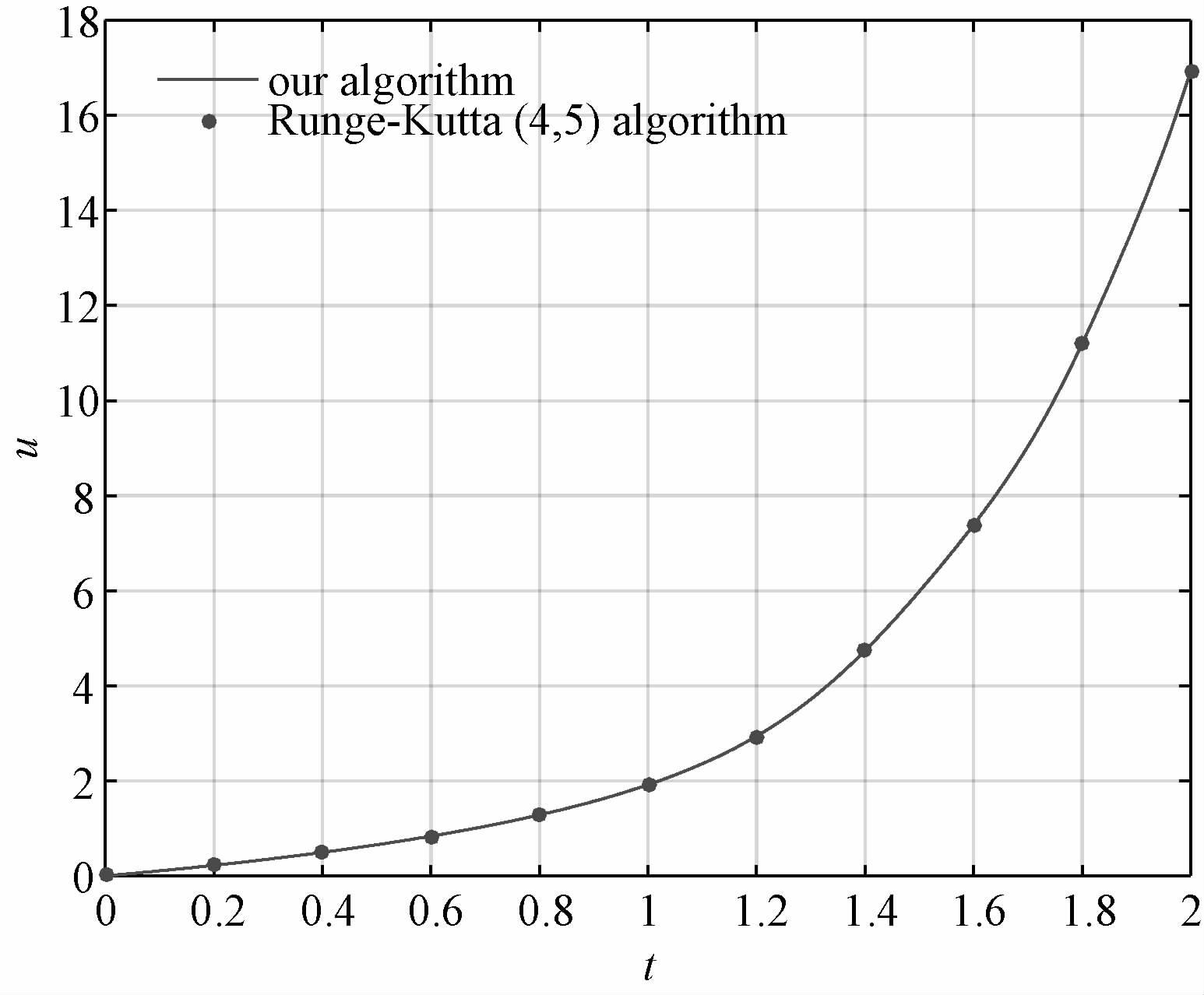
Figure 2 shows the difference between our algorithm and the Runge-Kutta algorithm. The red line indicates the solution of our algorithm and the blue points stand for Runge-Kutta algorithm.
Fig. 2

	Download: JPG larger image
Fig. 2 Difference between our algorithm and Runge-Kutta(4,5) algorithm

The errors for the specific points are given in Table 2. The results of our algorithm are in close proximity to the results of Runge-Kutta algorithm.
Table 2

Table 2 Results and relative errors of our algcrithm solution t ouralgorithm runge-Kutta algorithm relative error/% 0 0 0 0 0.2 0.221493 0.221492 0.000747 0.4 0.493722 0.493717 0.001062 0.6 0.835101 0.835088 0.001472 0.8 1.282323 1.282294 0.002284 1 1.917073 1.916985 0.00458 1.2 2.93768 2.937196 0.016479 1.4 4.740223 4.740419 -0.00415 1.6 7.384711 7.382598 0.028611 1.8 11.19865 11.20336 -0.04203 2 16.9337 16.93349 0.001268

Table 2 Results and relative errors of our algcrithm solution

4 ConclusionA new numerical solution is proposed and verified for the Volterra integral equation of the second kind. The established method would work with higher precision it one chooses a higher-precision numerical integration method. The proposed solution in this paper is easy to program and calculate, and the relative errors for the study cases are small enough. The limitation of the method is its dependence on the property of F-function.
References

[1]	Yusufoglu E. A homotopy perturbation algorithm to solve a system of Fredholm-Volterra type integral equations, 2008, 47:1099–1107.
[2]	Yusufoglu E. Numerical expansion methods for solving systems of linear integral equations using interpolation and quadrature rules, 2007, 84(1):133–149.
[3]	Huang L, Huang Y, Li X. Approximate solution of Abel integral equation, 2008, 56(7):1748–1757.
[4]	Yang C. Chebyshev polynomial solution of nonlinear integral equations, 2012, 349(3):947–956.
[5]	Yousefi S A. Numerical solution of Abel's integral equation by using Legendre wavelets, 2006, 175(1):574–580.
[6]	Khodabin M, Maleknejad K, Shekarabi F H. Application of triangular functions to numerical solution of stochastic Volterra integral equations, 2013, 43(1):1–9.
[7]	Kamyad A V, Mehrabinezhad M, Saberi-Nadjafi J. A numerical approach for solving linear and nonlinear Volterra integral equations with controlled error, 2010, 40(2):27–32.
[8]	Adomian G. Frontier problem of physics: the decomposition method[M].New York: Kluwer Academic Publish, 1994.
[9]	Bougoffa L, Rach R C, Mennouni A. A convenient technique for solving linear and nonlinear Abel integral equations by the Adomian decomposition method, 2011, 218(5):1785–1793.
[10]	Pandey R K, Singh O P, Singh V K. Efficient algorithms to solve singular integral equations of Abel type, 2009, 57(4):664–676.