蔡昕芮, 王丽瑾
中国科学院大学数学科学学院, 北京 100049
摘要: 提出3种基于离散观测数据的随机微分方程参数估计的方法。第1种方法应用于线性随机微分方程。推导出这类方程的真解的相关运算服从的分布，使观测数据的运算也服从此分布，由此来估计漂移系数与扩散系数中的未知参数。第2种方法用于It?型随机微分方程。推导出Euler-Maruyama格式的数值解的相关运算服从的分布，使观测数据的运算服从此分布，由此来估计参数。第3种方法用于Stratonovich型随机微分方程。推导出中点格式的数值解的相关运算服从的分布，使观测数据的运算服从此分布，以此来估计参数。数值实验验证了这3种方法的有效性。数值实验显示，Euler-Maruyama格式参数估计的误差约为O（h^0.5）阶，中点格式参数估计的误差约为O（h）阶，其中h是数值方法的时间步长。我们提出的3种估计方法均比文献中已有的EM-MLE方法更精确。
关键词: 随机微分方程参数估计Euler-Maruyama格式中点格式
Consider the stochastic differential equation (SDE)

$\begin{array}{*{20}{c}}{{\rm{d}}X\left( t \right) = f\left( {X\left( {\omega, t} \right), \theta } \right){\rm{d}}t + \sigma \left( {X\left( {\omega, t} \right), \gamma } \right){\rm{d}}B\left( t \right), }\\{X\left( {{t_0}} \right) = {X_0}, }\end{array}$

(1)

where t₀≤t≤T, and ω is an element of the underlying probability space Ω. f(·) and σ(·) are known functions of X, and B(t) is a standard Brownian motion. In addition, θ and γ are unknown parameters, which will be estimated. To simplify the exposition, we first assume that the parameters θ and γ are of one-dimension, and will present the discussion of estimating multiple unknown parameters in the last section. Moreover, we divide the time interval [t₀, T] into N pieces of equal length h, such that t_i+1-t_i=h, i=0, …, N-1, t_N=T.
The problem of parameter estimation in diffusion processes based on discrete observations has been studied by some authors. Morel et al.^[1] first studied estimation in discretely observed diffusions. Breton^[2] used approximate maximum likelihood estimation (MLE), and studied asymptotic properties of the descritized versions of MLE for linear parametric stochastic differential equations. Dorogovcev^[3] used conditional least squares estimation, and gave sufficient conditions for weak consistency of the estimator. Prakasa^[4] showed that Bayes estimators and MLE estimators of SDEs have the same asymptotic properties and asymptotic distributions for suitable class of loss functions of some special types. Combining statistical methods with numerical methods, Pedersen^[5] used numerical approximationsbased on iterations of the Gaussian transition densities emanating from Euler-Maruyama scheme and studied approximate maximum likelihood. Papaspiliopoulos and Beskos^[6] deduced the distribution of certain operation of the numerical solution of the stochastic differential equations by Euler-Maruyama scheme, and then used the maximum likelihood method to estimate the parameters based on observations, which we call the EM-MLE estimator. Inspired by their work, we propose estimators by deducing the distributions of certain relevant operations of the exact solution, as well as numerical solutions resulted from the Euler-Maruyama and the midpoint schemes of the SDEs. Instead of the maximum likelihood method in Ref.[6], we use directly the deduced distributions together with tree-like observations to estimate the parameters. Errors of our estimators are compared with that of the EM-MLE estimator in the numerical experiments.
The contents are arranged as follows. In section 1, we derive the distribution of an operation of the exact solution of constant-coefficient homogeneous linear SDE, and deseribe the method of parameter estimation based on this distribution. In section 2 we propose two methods of parameter estimation for SDEs of It${\hat o}$ and Stratonovich senses, respectively, based on the distribution of corresponding operations of the numerical solutions produced by the Euler-Maruyama scheme and the midpoint scheme, respectively. In section 3, we perform numerical experiments to test these methods, and estimate the order of errors arising from the latter two methods. Error comparison with the EM-MLE estimator is also performed. Section 4 is devoted to the discussion of estimating multiple unknown parameters for SDEs, based on the Euler-Maruyama numerical scheme.
1 Method based on the exact solutionConsider the constant-coefficient homogeneous linear SDE

$\begin{array}{*{20}{c}}{{\rm{d}}X\left( t \right) = aX\left( t \right){\rm{d}}t + bX\left( t \right){\rm{d}}B\left( t \right), }\\{X\left( 0 \right) = {X_0} \ne 0, }\end{array}$

(2)

where a and b are unknown parameters. The exact solution of this SDE has the form

$X\left( t \right) = {X_0}\exp \left[{\left( {a-\frac{1}{2}{b^2}} \right)t + bB\left( t \right)} \right].$

(3)

Obviously,

$X\left( {{t_i}} \right) = {X_0}\exp \left[{\left( {a-\frac{1}{2}{b^2}} \right){t_i} + bB\left( {{t_i}} \right)} \right], $

(4)

$X\left( {{t_{i + 1}}} \right) = {X_0}\exp \left[{\left( {a-\frac{1}{2}{b^2}} \right){t_{i + 1}} + bB\left( {{t_{i + 1}}} \right)} \right].$

(5)

From (4) and (5), it follows

$\begin{array}{l}X\left( {{t_{i + 1}}} \right) = X\left( {{t_i}} \right)\exp \left[{\left( {a-\frac{1}{2}{b^2}} \right)h + } \right.\\\;\;\;\;\;\;\;\;\;\;\;\;\;\;\;\left. {b\left( {B\left( {{t_{i + 1}}} \right)-B\left( {{t_i}} \right)} \right)} \right], \end{array}$

(6)

where h=t_i+1-t_i, and

$B\left( {{t_{i + 1}}} \right) - B\left( {{t_i}} \right)\tilde{\ }N\left( {0, h} \right).$

Therefore,

$\begin{array}{l}\;\;\;\;\;\;\;\;\ln\left| {X\left( {{t_{i + 1}}} \right)} \right| - \ln\left| {X\left( {{t_i}} \right)} \right|\\ = \left( {a - \frac{1}{2}{b^2}} \right)h + b\left( {B\left( {{t_{i + 1}}} \right) - B\left( {{t_i}} \right)} \right)\\ \sim N\left( {\left( {a - \frac{1}{2}{b^2}} \right)h, {b^2}h} \right).\end{array}$

(7)

Suppose we have observations

$\begin{array}{*{20}{c}}{X\left( {{\omega _1}, {t_0}} \right), X\left( {{\omega _1}, {t_1}} \right), \cdots, X\left( {{\omega _1}, {t_N}} \right), }\\ \vdots \\{X\left( {{\omega _m}, {t_0}} \right), X\left( {{\omega _m}, {t_1}} \right), \cdots, X\left( {{\omega _m}, {t_N}} \right), }\end{array}$

where ω_j ∈ Ω, X(ω_j, t₀)=X₀, for j=1, …, m.
On the first subinterval [t₀, t₁], we calculate

$\begin{array}{*{20}{c}}{\ln \left| {X\left( {{\omega _1}, {t_1}} \right)} \right| - \ln \left| {X\left( {{\omega _1}, {t_0}} \right)} \right|, }\\{\ln \left| {X\left( {{\omega _2}, {t_1}} \right)} \right| - \ln \left| {X\left( {{\omega _2}, {t_0}} \right)} \right|, }\\ \vdots \\{\ln \left| {X\left( {{\omega _m}, {t_1}} \right)} \right| - \ln \left| {X\left( {{\omega _m}, {t_0}} \right)} \right|.}\end{array}$

(8)

According to the method of moments, we can approximate the total moments by the moments of the samples. Therefore, let

$\begin{array}{*{20}{l}}{\left( {a - \frac{1}{2}{b^2}} \right)h = \frac{1}{m}\sum\limits_{j = 1}^m {\ln \left| {X\left( {{\omega _1},{t_1}} \right)} \right|} - }\\{\;\;\;\;\;\;\;\;\;\;\;\;\;\;\;\;\;\;\;\;\ln \left| {(X\left( {{\omega _j},{t_0}} \right)} \right|,}\\{{b^2}h = \frac{1}{{m - 1}}\sum\limits_{j = 1}^m {(\ln \left| {X\left( {{\omega _i},{t_1}} \right)} \right|} - }\\{\;\;\;\;\;\;\;\;{{\left. {\ln \left| {X\left( {{\omega _j},{t_0}} \right)} \right| - \left( {a - \frac{1}{2}{b^2}} \right)h} \right)}^2}}\end{array}$

to get the estimator of a and b on the first subinterval [t₀, t₁], denoted by a ${\hat a_1}$ and ${\hat b_1}$.
By performing the same procedure on the subsequent small intervals [t₁, t₂], …, [t_N-1, t_N], we get a sequence of estimators $ {\hat a_2}, \cdots, {\hat a_N}$ and ${\hat b_2}, \cdots, {\hat b_N}$. Then, we estimate the parameter a by the average of $ {\hat a_1}, \cdots, {\hat a_N}$, and estimate b by the average of ${\hat b_1}, \cdots, {\hat b_N}$, that is

$\hat a = \frac{1}{N}\sum\limits_{i = 1}^N {{{\hat a}_i}}, \hat b = \frac{1}{N}\sum\limits_{i = 1}^N {{{\hat b}_i}} .$

(9)

2 Methods based on the numerical solutionsIn this section, we will give parameter estimators based on two kinds of numerical discretizations of the SDEs containing unknown parameters.
2.1 Method using the Euler-Maruyama schemeConsider the SDE of It${\hat o}$ sense (1). Denote by X_i the numerical solution at time t_i. The Euler-Maruyama scheme^[7] applied to (1) reads

${X_{i + 1}} - {X_i} = hf\left( {{X_i}, \theta } \right) + \left[{B\left( {{t_{i + 1}}} \right)-B\left( {{t_i}} \right)} \right]\sigma \left( {{X_i}, \gamma } \right).$

(10)

Given X_i, we know that the distribution of the increment is

${X_{i + 1}} - {X_i} \sim N\left( {hf\left( {{X_i}, \theta } \right), h{\sigma ^2}\left( {{X_i}, \gamma } \right)} \right).$

(11)

Suppose we have m observations X(ω₁⁰, t₁), X(ω₂⁰, t₁), …, X(ω_m⁰, t₁), each appearing after evolution of a time period h from the given initial value X₀. Then due to (11), we can let

$\frac{1}{m}\sum\limits_{j = 1}^m {X\left( {\omega _j^0, {t_1}} \right)} = hf\left( {{X_0}, \theta } \right) + {X_0}$

and

$\frac{1}{{m - 1}}\sum\limits_{j = 1}^m {{{\left( {X\left( {\omega _j^0, {t_1}} \right) - hf\left( {{X_0}} \right)} \right)}^2}} = h{\sigma ^2}\left( {{X_0}, \gamma } \right), $

from which we get an estimate ${{\hat \theta }_1}$ and ${{\hat \gamma }_1}$.
Then, we fix an arbitrary X(ω_k⁰, t₁)=:X₁ (k ∈ {1, …, m}), and observe other m values X(ω₁¹, t₂), X(ω₂¹, t₂), …, X(ω_m¹, t₂), each resulting from evolving time h from the given value X(ω_k⁰, t₁)=X₁. Let

$\frac{1}{m}\sum\limits_{j = 1}^m {X\left( {\omega _j^1, {t_2}} \right)} = hf\left( {{X_1}, \theta } \right) + {X_1}, $

and

$\frac{1}{{m - 1}}\sum\limits_{j = 1}^m {{{\left( {X\left( {\omega _j^1, {t_2}} \right) - hf\left( {{X_1}} \right)} \right)}^2}} = h{\sigma ^2}\left( {{X_1}, \gamma } \right).$

We obtain another estimate ${{\hat \theta }_2}$ and ${{\hat \gamma }_2}$.
Analogously, we can get successively a sequence of estimates ${{\hat \theta }_3}, \cdots, {{\hat \theta }_N}$ and ${{\hat \gamma }_3}, \cdots, {{\hat \gamma }_N}$. Then we use the average of $ {{\hat \theta }_i}$, i=1, …, N, to estimate the parameter θ and use the average of ${{\hat \gamma }_i}$, i=1, …, N, to estimate the parameter γ. That is

$\hat \theta = \frac{1}{N}\sum\limits_{i = 1}^N {{{\hat \theta }_i}}, \hat \gamma = \frac{1}{N}\sum\limits_{i = 1}^N {{{\hat \gamma }_i}} .$

(12)

2.2 Method using the midpoint schemeFor the SDE of Stratonovich sense

$\begin{array}{*{20}{c}}{{\rm{d}}X\left( t \right) = f\left( {X\left( {\omega, t} \right), \theta } \right){\rm{d}}t + \sigma \left( {X\left( {\omega, t} \right), \gamma } \right) \circ {\rm{d}}B\left( t \right), }\\{X\left( {{t_0}} \right) = {X_0}, }\end{array}$

(13)

the midpoint scheme is a kind of consistent numerical method (see Ref.[7]). If θ and γ are unknown parameters, we apply the midpoint scheme to (13), and simulate B(t_i+1)-B(t_i) by ${\xi _i}\sqrt h $, where ξ_i is a random variable of standard normal distribution. We get

$\begin{array}{l}{X_{i + 1}} - {X_i} = f\left( {\frac{{{X_{i + 1}} + {X_i}}}{2}, \theta } \right)h + \\\;\;\;\;\;\;\;\;\;\;\;\;\;\;\;\;\;\;\sigma \left( {\frac{{{X_{i + 1}} + {X_i}}}{2}, \gamma } \right){\xi _i}\sqrt h .\end{array}$

(14)

Since scheme (14) is usually implicit, we may need to use predictor-corrector type iterations, as well as proper truncation of the ξ_i to compute an approximation ${{\tilde X}_{i + 1}}$ of X_i+1. Then we have

$\frac{{{{\tilde X}_{i + 1}} - {X_i} - f\left( {\frac{{{{\tilde X}_{i + 1}} + {X_i}}}{2}, \theta } \right)h}}{{\sigma \left( {\frac{{{{\tilde X}_{i + 1}} + {X_i}}}{2}, \gamma } \right)\sqrt h }} \approx {\xi _i} \sim N\left( {0, 1} \right), $

(15)

where X_i is given by last iteration step.
We use the same observation as described in section 2.1. According to (15), for the first time interval [t₀, t₁], we can let

$\begin{array}{*{20}{c}}{\frac{1}{m}\sum\limits_{j = 1}^m {\frac{{X\left( {\omega _j^0, {t_1}} \right) - {X_0} - f\left( {\frac{{X\left( {\omega _j^0, {t_1}} \right) + {X_0}}}{2}, \theta } \right)}}{{\sigma \left( {\frac{{X\left( {\omega _j^0, {t_1}} \right) + {X_0}}}{2}, \gamma } \right)\sqrt h }} = 0, } }\\{\frac{1}{{m - 1}}\sum\limits_{j = 1}^m {{{\left( {\frac{{X\left( {\omega _j^0, {t_1}} \right) - {X_0} - f\left( {\frac{{X\left( {\omega _j^0, {t_1}} \right) + {X_0}}}{2}, \theta } \right)h}}{{\sigma \left( {\frac{{X\left( {\omega _j^0, {t_1}} \right) + {X_0}}}{2}, \gamma } \right)\sqrt h }}} \right)}^2}} }\\{ = 1, }\end{array}$

from which we can get an estimate ${{\hat \theta }_1}$ and ${{\hat \gamma }_1}$. Performing the same procedure for the time intervals [t₁, t₂], …, [t_N-1, t_N], we obtain a sequence of estimates ${{\hat \theta }_2}, \cdots, {{\hat \theta }_N}$ and $ {{\hat \gamma }_2}, \cdots, {{\hat \gamma }_N}$. We estimate θ and γ by

$\hat \theta = \frac{1}{N}\sum\limits_{i = 1}^N {{{\hat \theta }_i}}, \hat \gamma = \frac{1}{N}\sum\limits_{i = 1}^N {{{\hat \gamma }_i}} .$

(16)

Alternatively, we can transform the SDE of Stratonovich sense (13) into its equivalent It${\hat o} $ form

$\begin{array}{*{20}{c}}{{\rm{d}}X\left( t \right) = \left( {f\left( {X\left( {\omega, t} \right), \theta } \right) + \frac{1}{2}\frac{{\partial \sigma }}{{\partial X}} \cdot } \right.}\\{\left. {\sigma \left( {X\left( {\omega, t} \right), \gamma } \right)} \right){\rm{d}}t + \sigma \left( {X\left( {\omega, t} \right), \gamma } \right){\rm{d}}B\left( t \right), }\\{X\left( {{t_0}} \right) = {X_0}, }\end{array}$

(17)

and then use the method given in section 2.1 to estimate the parameters. We will compare the results of the two approaches based on Stratonovich and It${\hat o} $ equations, respectively, by numerical tests as follows.
3 Numerical tests3.1 Estimation based on the exact solutionFor the linear SDE (2), let t₀=0, T=1, X₀=1. Suppose a and b are given. a and b will be estimated by using the method given in section 1 to test the ability of our estimator.We set the number of subintervals of time to be N=500 and the number of sample path observations to be m=100, and we perform five tests for five different groups of a and b values. The observation data are simulated by the exact solution (3). Our five group of numerical results ${\hat a}$ and ${\hat b}$, with the corresponding a and b, are listed in Table 1.
Table 1

Table 1 Estimates based on the exact solution a b ${\hat a}$ ${\hat b}$ 1 0.5 0.984 2 0.497 7 2 2 2.018 9 1.994 7 3 1 2.984 7 1.004 1 4 2 4.025 5 1.992 3 5 3 5.010 9 2.995 8

Table 1 Estimates based on the exact solution

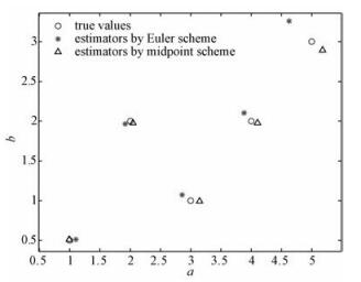
In Fig. 1(a), we plot the points (a, b) denoted by 'o', and the corresponding estimates ($\hat a, \hat b$) denoted by '*' in the five tests. Fig. 1(a) shows very good coincidence between the exact value and the estimates.
Fig. 1

	Download: JPG larger image
Fig. 1 Exact values and estimates of the parameter (a, b)

3.2 Estimation based on the numerical solutionsTo test the effect of the parameter estimations based on the Euler-Maruyama and the midpoint schemes, we first consider the linear SDE of Stratonovich sense

$\begin{array}{*{20}{c}}{{\rm{d}}X\left( t \right) = aX\left( t \right){\rm{d}}t + bX\left( t \right) \circ {\rm{d}}B\left( t \right), }\\{X\left( 0 \right) = {X_0} \ne 0, }\end{array}$

(18)

and its equivalent It${\hat o}$ equation

$\begin{array}{*{20}{c}}{{\rm{d}}X\left( t \right) = \left( {a + \frac{1}{2}{b^2}} \right)X\left( t \right){\rm{d}}t + bX\left( t \right){\rm{d}}B\left( t \right), }\\{X\left( 0 \right) = {X_0} \ne 0.}\end{array}$

(19)

We apply the midpoint scheme to (18) and the Euler-Maruyama scheme to (19). Then we compare their effects.
The data are set as t₀=0, T=1, X₀=1, N=100, and m=500, and the observation data are generated by the exact solution of (18) and (19)

$X\left( t \right) = {X_0}\exp \left( {at + bB\left( t \right)} \right).$

(20)

Again, we perform five tests with five different groups (a, b), and denote the estimates by the Euler-Maruyama scheme with (${{\hat a}_e}, {{\hat b}_e}$) and that by the midpoint scheme with ($ {{\hat a}_m}, {{\hat b}_m}$). The numerical results are listed in Table 2.
Table 2

Table 2 Estimates based on the numerical solutions a b ${{\hat a}_e}$ ${{\hat b}_e}$ $ {{\hat a}_m}$ ${{\hat b}_m}$ 1 0.5 1.045 1 0.506 2 1.040 7 0.499 9 2 2 1.927 8 2.097 6 2.035 6 1.975 6 3 1 3.039 3 1.034 7 3.007 7 0.994 5 4 2 3.989 3 2.140 8 4.063 1.974 6 5 3 4.579 8 3.391 7 5.206 6 2.937 8

Table 2 Estimates based on the numerical solutions

In Fig. 1(b) we plot the five points (a, b) denoted by 'o', and the corresponding estimates (${{\hat a}_e}, {{\hat b}_e}$) denoted by '*' and (${{\hat a}_m}, {{\hat b}_m}$) denoted by '△'. It can be seen that the midpoint scheme applied to the Stratonovich SDE gives better estimates than the Euler-Maruyama scheme applied to the It${\hat o}$ SDE.
3.3 Error analysisIn this section, we analyze the relation between the error of estimate $e: = \sqrt {{{\left( {a-\hat a} \right)}^2} + {{\left( {b-\hat b} \right)}^2}} $ and the time step size h of the numerical solutions using the Euler-Maruyama scheme and the midpoint scheme. Consider the linear SDE of It${\hat o}$ sense (19) and its equivalent SDE of Stratonovich sense (18), for which we apply the Euler-Maruyama scheme and the midpoint scheme, respectively.
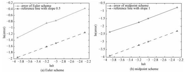
Set X₀=1, t₀=0, T=1, a=3, b=1, and the number of observed sample paths m=500. We test four different values of the time step size of the numerical solutions, namely, h=0.02, 0.04, 0.05, and 0.1. In Table 3 listed are the estimated values (${{\hat a}_e}, {{\hat b}_e}$) resulted from the Euler-Maruyama scheme and (${{\hat a}_m}, {{\hat b}_m}$) resulted from the midpoint scheme, together with the corresponding time step sizes h.
Table 3

Table 3 Estimates and the corresponding h values h a b $ {{\hat a}_e}$ $ {{\hat b}_e}$ $ {{\hat a}_m}$ $ {{\hat b}_m}$ 0.02 3 1 3.062 6 1.075 1 3.001 6 0.990 9 0.04 3 1 3.060 7 1.173 5 2.952 4 0.993 3 0.05 3 1 3.055 6 1.182 8 2.913 8 0.974 2 0.1 3 1 3.125 1.476 7 2.911 0.966 6

Table 3 Estimates and the corresponding h values

In Table 3, we observe an inereasing tendency of errore with h for both numerical schemes. For a clearer demonstration, we plot lne against lnh for the four different values of h and the corresponding errors e in Fig. 2, with Fig. 2(a) for the Euler-Maruyama scheme and Fig. 2(b) for the midpoint scheme. In Fig. 2, we can observe the order of the error with respect to h. The dashed reference line in Fig. 2(a) is of slope 0.5. The near parallelism between the reference line and the plotted lne-lnh line indicates that the order of the error e for the Euler-Maruyama scheme is about O(h^0.5). Analogously, it can be inferred from Fig. 2(b) that the error e for the midpoint scheme is of order O(h), since the dashed reference line in Fig. 2(b) is of slope 1.
Fig. 2

	Download: JPG larger image
Fig. 2 Error orders with respect to h

Meanwhile, it is interesting to note that the Euler-Maruyama method applied to the SDE (19) is of root mean-square convergence order 0.5, while the midpoint scheme applied to the SDE (18) is of root mean-square convergence order 1 ([7, 8]). Three facts imply that the estimate errors based on the numerical solutions may mainly result from the error of the numerical methods themselves. More accurate estimators might be obtained by applying higher-order numerical methods.
3.4 Error comparison with the EM-MLE estimatorFor the linear SDE (2), we apply our estimator based on the exact solution, which we call the exact solution estimator, and the EM-MLE estimator [6] to estimate the parameters (a, b), which are given as a=3, b=1. Moreover, set X₀=1, t₀=0, and T=1. We perform four tests with four different values of h, namely, h=0.02, 0.04, 0.05, and 0.1, and observe m=100 sample paths for each. Denote the estimate arising from our method by ($\hat a, \hat b$), and its error by $e: = \sqrt {{{\left( {a-\hat a} \right)}^2} + {{\left( {b-\hat b} \right)}^2}} $, and those from the EM-MLE estimator by (${{\hat a}_M}, {{\hat b}_M}$) and ${e_M}: = \sqrt {{{\left( {a-{{\hat a}_M}} \right)}^2} + {{\left( {b-{{\hat b}_M}} \right)}^2}} $, respectively. In Table 4 listel are the numerical results.
Table 4

Table 4 Exact solution and EM-MLE estimators h ${\hat a}$ ${\hat b}$ ${{{\hat a}_M}}$ ${{{\hat b}_M}}$ e ${{{\hat e}_M}}$ 0.02 3.048 1.101 3.329 1.122 0.049 0.351 0.04 2.925 1.006 2.505 1.049 0.074 0.497 0.05 2.901 0.985 2.492 1.238 0.099 0.560 0.1 3.109 6 1.017 4.578 1.044 0.110 1.579

Table 4 Exact solution and EM-MLE estimators

Table 4 shows that our exact solution estimator is more accurate than the EM-MLE estimator.
To compare our numerical solution estimators with the EM-MLE estimator, we consider the linear SDE of Stratonovich sense (18), to which we apply the midpoint scheme estimator, and the equivalent It${\hat o}$ SDE (19), for which we use the Euler-Maruyama estimator and the EM-MLE estimator. Set a=3, b=1, X₀=1, t₀=0, and T=1. Again we perform four tests with h=0.02, 0.04, 0.05, and 0.1, respectively, and m=100 for each.
In Table 5, (${{\hat a}_e}, {{\hat b}_e}$), (${{\hat a}_m}, {{\hat b}_m}$), and (${{\hat a}_M}, {{\hat b}_M}$) denote the estimates arising from the Euler-Maruyama, midpoint, and the EM-MLE estimators, respectively, and e_e, e_m, and e_M represent their errors, respectively. It is obvious that our numerical solution estimators are more accurate than the EM-MLE estimator as well.
Table 5

Table 5 Numerical solution and EM-MLE estimators h ${{\hat a}_e}$ ${{\hat b}_e}$ ${{\hat a}_m}$ ${{\hat b}_m}$ ${{\hat a}_M}$ ${{\hat b}_M}$ ee em eM 0.02 3.007 1.134 3 2.972 7 0.981 7 2.990 8 0.889 5 0.134 4 0.032 9 0.110 9 0.04 3.113 1.075 1 3.05 0.990 8 3.414 1.006 9 0.135 7 0.050 9 0.414 0.05 3.103 9 1.214 7 2.893 9 0.973 8 2.250 9 0.984 2 0.238 5 0.109 3 0.749 3 0.1 2.955 6 1.5093 2.829 9 0.968 4.414 3 1.094 9 0.511 2 0.173 1 1.417 5

Table 5 Numerical solution and EM-MLE estimators

3.5 Numerical tests on non-linear SDEsTo test the effect of our estimators on non-linear SDEs, we consider the following SDE

$\begin{array}{*{20}{c}}{X\left( t \right) = a{X^2}\left( t \right){\rm{d}}t + b{X^2}\left( t \right) \circ {\rm{d}}B\left( t \right), }\\{X\left( {{t_0}} \right) = {X_0}, }\end{array}$

(21)

and its equivalent It${\hat o}$ form

$X\left( t \right) = \left( {a{X^2}\left( t \right) + {b^2}{X^3}\left( t \right)} \right){\rm{d}}t + b{X^2}\left( t \right){\rm{d}}B\left( t \right), $

(22)

where a and b are unknown parameters to be estimated.
We apply the midpoint estimator to (21), and the Euler-Maruyama estimator to (22). Set X₀=0.5, t₀=0, T=1, and h=0.02. We use the midpoint scheme with tiny step size h=0.001 to (21) to simulate the true solution of the system which serves as observation data for our tests, and we conduct m=500 samples. The estimation results with different sets of a and b are listed in Table 6, where ${{\hat a}_e} $ and ${{\hat b}_e}$ are from the Euler-Maruyama estimator and ${{\hat a}_m}$ and $ {{\hat b}_m}$ are from the midpoint estimator.
Table 6

Table 6 Estimates with different a and b values a b ${{\hat a}_e}$ ${{\hat b}_e}$ ${{\hat a}_m}$ ${{\hat b}_m}$ 1 0.5 1.103 0.511 8 0.992 4 0.510 2 2 2 1.917 3 1.965 3 2.045 1 1.976 7 3 1 2.858 1.072 8 3.146 3 0.992 2 4 2 3.881 4 2.103 8 4.104 5 1.978 1 5 3 4.627 7 3.260 2 5.179 4 2.893 6

Table 6 Estimates with different a and b values

Again, we plot the five groups of points (a, b), (${{\hat a}_e}, {{\hat b}_e}$), and (${{\hat a}_m}, {{\hat b}_m}$) in Fig. 3. It can be seen that the midpoint estimator is more accurate than the Euler-Maruyama estimator.
Fig. 3

	Download: JPG larger image
Fig. 3 Exact values and estimates of the parameter (a, b) in the nonlinear SDE (21) or (22)

Then, we fixa=1 and b=2, but take h=0.02, 0.04, 0.05, and 0.1, to observe the order of the error $e: = \sqrt {{{\left( {a-\hat a} \right)}^2} + {{\left( {b-\hat b} \right)}^2}} $ of the estimators with respect to h. Once more we set X₀=0.5, t₀=0, T=1, and m=500. The numerical results are given in Table 7, where the items with lower-index e are from the Euler-Maruyama estimator, while those with m are from the midpoint estimator.
Table 7

Table 7 Estimates and errors h ${{\hat a}_e}$ ${{\hat b}_e}$ ${{\hat a}_m}$ ${{\hat b}_m}$ ee em 0.02 1.048 9 2.060 4 0.998 2 1.986 5 0.077 7 0.013 6 0.04 1.076 2 2.098 5 0.981 4 1.960 2 0.124 5 0.043 9 0.05 1.105 3 2.185 6 0.974 2 1.897 8 0.213 4 0.105 4 0.1 1.174 2.260 2 1.158 3 2.144 7 0.313 0.214 5

Table 7 Estimates and errors

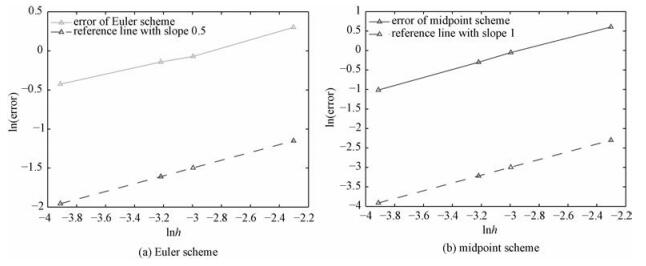
Figure 4(a) and Fig. 4(b) illustrate the ln|error| ~ ln h relationships arising from the Euler-Maruyama and the midpoint estimator, respectively.
Fig. 4

	Download: JPG larger image
Fig. 4 Error orders with respect to h of non-linear SDE estimators

It is indicated that for the non-linear SDE (22) or its equivalent equation (21), the order of the error e_e produced by the Euler-Maruyama estimator is about O(h^0.5) while that by the midpoint estimator is about O(h). This is the same as the indication for the numerical results for the linear SDE in the previous subsections.
3.6 A remarkIt is observed from the above-performed numerical tests that, with the growth of the order of the numerical method, the estimation accuracy is improved. It is then naturally expected that higher order methods give better estimations. However, in high-order stochastic numerical schemes such as the weak order 2 It${\hat o}$ -Taylor scheme (see e.g., Ref.[7]), high order multiple stochastic integrals such as $\int\limits_{{t_n}}^{{t_{n + 1}}} {\int_{{t_n}}^s {{\rm{d}}B\left( u \right){\rm{d}}s} } $ will appear, together with B(t_n+1)-B(t_n), where B(t) denotes the standard Brownian motion. It therefore becomes complicated to derive an appropriate calculation with certain distribution from the numerical scheme. Nevertheless, this could be an interesting topic deserving further investigations.
4 Estimating multiple parametersUp to now we have considered estimation of 2 unknown parameters appearing in the drift and diffusion coefficients of a SDE. Actually, our methods can be extended to estimate multiple unknown parameters. Consider the following SDE

$\begin{array}{*{20}{c}}{{\rm{d}}X\left( t \right) = f\left( {X\left( {\omega, t} \right), {\theta _1}, \cdots, {\theta _p}} \right){\rm{d}}t + }\\{\sigma \left( {X\left( {\omega, t} \right), {\gamma _1}, \cdots, {\gamma _q}} \right){\rm{d}}B\left( t \right), }\\{X\left( {{t_0}} \right) = {X_0}, }\end{array}$

(23)

where θ₁, …, θ_p, γ₁, …, γ_q are (p+q) unknown parameters to be estimated. Applying the Euler-Maruyame scheme to the SDE (23), we have

${X_{i + 1}} - {X_i} \sim N\left( {hf\left( {{X_i}, \Theta } \right), h{\sigma ^2}\left( {{X_i}, \Gamma } \right)} \right), $

(24)

where Θ:=(θ₁, …, θ_p), Γ:=(γ₁, …, γ_q).
Given m observations at time $ {t_1} = {t_0} + h, X\left( {\omega _1^0, {t_1}} \right), X\left( {\omega _2^0, {t_1}} \right), \cdots, X\left( {\omega _m^0, {t_1}} \right)$, we let

$\begin{array}{*{20}{c}}{\frac{1}{m}\sum\limits_{j = 1}^m {X\left( {\omega _j^0, {t_1}} \right)} = hf\left( {{X_0}, \Theta } \right) + {X_0}, }\\{\frac{1}{{m - 1}}\sum\limits_{j = 1}^m {{{\left( {X\left( {\omega _j^0, {t_1}} \right) - {X_0} - hf\left( {{X_0}, \Theta } \right)} \right)}^2}} }\\{ = h{\sigma ^2}\left( {{X_0}, \Gamma } \right), }\\{\frac{1}{m}\sum\limits_{j = 1}^m {X{{\left( {\omega _j^0, {t_1}} \right)}^3}} = E\left( {X_1^3} \right) = \int\limits_{ - \infty }^{ + \infty } {{x^3}{\rho _1}\left( x \right){\rm{d}}x}, }\\ \vdots \\{\frac{1}{m}\sum\limits_{j = 1}^m {X{{\left( {\omega _j^0, {t_1}} \right)}^{p + q}}} = E\left( {X_1^{p + q}} \right) = \int\limits_{ - \infty }^{ + \infty } {{x^{p + q}}{\rho _1}\left( x \right){\rm{d}}x}, }\end{array}$

(25)

where ${\rho _1}\left( x \right) = \frac{1}{{\sqrt {2{\rm{\pi }}} {d_1}}}\exp \left( {-\frac{{{{\left( {x-{c_1}} \right)}^2}}}{{2d_1^2}}} \right) $, with c₁:=hf(X₀, Θ)+X₀, d₁²:=h σ²(X₀, Γ). The E(X₁^k) (k=3, …, p+q) can be calculated in terms of the characteristic function of X₁, that is,

$\begin{array}{l}g\left( t \right) = E{{\rm{e}}^{{\rm{i}}t{X_1}}} = \frac{1}{{\sqrt {2{\rm{\pi }}} {d_1}}}\int\limits_{ - \infty }^{ + \infty } {{{\rm{e}}^{{\rm{i}}tx}}\exp \left( { - \frac{{{{\left( {x - {c_1}} \right)}^2}}}{{2d_1^2}}} \right){\rm{d}}x} \\\;\;\;\;\;\;\; = {{\rm{e}}^{{\rm{i}}{c_1}t - \frac{{d_1^2{t^2}}}{2}}}, \end{array}$

(26)

with the property that the k-th derivative of g at t=0 is g^(k)(0)=i^kE(X₁^k).
There are (p+q) unknowns and (p+q) equations in the equations system (25), which is usually non-linear and might need iteration methods for solving the unknowns $\hat \theta _1^1, \cdots, \hat \theta _p^1, \hat \gamma _1^1, \cdots, \hat \gamma _q^1$.
Given observations at time t₂=t₀+2h, …, t_N=t₀+Nh, we write similar equations systems regarding the p+q moments of X_i with probability density function ${\rho _i}\left( x \right) = \frac{1}{{\sqrt {2{\rm{\pi }}} {d_i}}}\exp \left( {-\frac{{{{\left( {x-{c_i}} \right)}^2}}}{{2d_i^2}}} \right) $, where c_i=hf(X_i-1, Θ)+X_i-1, d_i²=hσ²(X_i-1, Γ), for i=2, …, N, and get the corresponding estimations $\hat \theta _1^2, \cdots, \hat \theta _p^2, \hat \gamma _1^2, \cdots, \hat \gamma _q^2, \cdots, \hat \theta _1^N, \cdots, \hat \theta _p^N, \hat \gamma _1^N, \cdots, \hat \gamma _q^N $. Then we set

${{\hat \theta }_i} = \frac{1}{N}\sum\limits_{l = 1}^N {\hat \theta _i^l}, {{\hat \gamma }_i} = \frac{1}{N}\sum\limits_{l = 1}^N {\hat \gamma _i^l}, $

(27)

for i=1, …, p, j=1, …, q.
Note that the observation data are the same tree-like data as described in section 3.1, wherefore the X_i is known when we calculate the moments of X_i+1, for i=0, …, N-1.
References

[1]	Morel J M, Takens F, Teissier B. Parameter estimation in stochastic differential equations[M].Berlin Heidelberg: Springer-Verlag, 2008: 6-10.
[2]	Breton A L. On continuous and discrete sampling for parameter estimation in diffusion type processes[M].Berlin Heidelberg: Springer, 1976: 124-144.
[3]	Dorogovcev A J. The asymptotic properties of least square estimators for regression coefficients[J].Problemy Peredai Informacii, 1973, 4:49–57.
[4]	Prakasa R. On Bayes estimation for diffusion fields[M].North Holland: Statistical Publishing Society, 1984: 575-590.
[5]	Pedersen A R. A new approach to maximum likelihood estimation for stochatic differential equations based on discrete observations[J].Scandinavian Journal of Statistics, 1995, 22(1):55–71.
[6]	Papaspiliopoulos O, Beskos A. An introduction to modelling and likelihood inference with stochastic differential equations. Great Britain: Warwick, 2011.
[7]	Kloeden P E, Platen E. Numerical solution of stochastic differential equations[M].Berlin Heidelberg: Springer-Verlag, 1992: 305.
[8]	Milstein G N, Tretyakov M V. Stochastic numerics for mathematical physics[M].Berlin Heidelberg: Springer, 2004: 9-10.