
中国科学院大学物理科学学院, 北京 101408
摘要: 反弹暴涨成功解决了暴涨无法解决的奇点问题。一般地,该模型反弹区域持续时间较短。着重讨论宽反弹情形,并研究宽反弹期间的引力波功率谱。
关键词: 反弹暴涨引力波功率谱
Inflation[1-3], as the paradigm of the early universe, is a fundamental model of the cosmology. It has not only solved the problems of the big bang theory but also provided the primordial scalar and tensor perturbations that generate the large-scale structure[4]. However, because of the so-called "singularity problem", inflation theory needs to be improved. An acceptable way to solve the problem is considering the so-called bounce inflation scenario[5-7](see also Refs.[8-17]). In bounce inflation, there is a contracting phase after a bounce phase the inflation starts. Recently, the development of effective field theory of nonsingular cosmologies[18-20] has made us construct full stable bounce models.
The evidence, that is, the power deficit of the CMB TT-mode spectrum at large scale observed by the Plank collaboration makes physicists to consider the physics before inflation[21]. The bounce model is accepted by many workers in order to solve the problem above, which has been reviewed in Refs.[22-23].
Primordial gravitational waves (GWs) open an important window for exploring the early universe. Recently, a large number of experiments aiming at observing GWs have been implemented or will be implemented[24]. Thus understanding about the early universe and inflation scenario will be deeper and deeper. Since the primordial GWs are independent of the dynamics of the scalar field, it can be used to identify the physics of the pre-inflation background. In a previous work[25], GWs of bounce model has been studied, in which the duration that the bounce lasts is short (the so-called narrow bounce). However, the case of broad bounce is not ruled out. In this study, we focus on the GWs from the bounce inflation with a broad bounce.
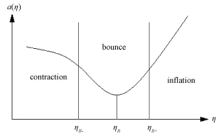
1 Tensor perturbation in bounce inflation scenarioIn bounce inflation scenario, the universe experiences a phase, showed in Fig. 1, before inflation, in which a varying with η is the scale factor of the universe, ηB- is the beginning time of bounce phase, ηB is the so-called bounce point at which Hubble Constant H=0, and ηB+ is the ending time of bounce phase. By contrast to the previous work, contracting phase does not keep symmetric to inflation, which also means HB-≠-HB+.
Fig. 1
 | Download: JPG larger image |
ηB is the so-called bounce point. Fig. 1 The bounce phase occurring between ηB- and ηB+ | |
We start with the second order perturbation action in which tensor perturbation γij presents the physical message in this time,
| $S_{{\gamma _{ij}}}^{\left( 2 \right)} = \int {{d^4}x{a^2}\left[ {{{\left( {{{\gamma '}_{ij}}} \right)}^2} - {{\left( {\partial {{\gamma '}_{ij}}} \right)}^2}} \right]} .$ | (1) |
| ${u''_k} + \left( {{k^2} - \frac{{a''}}{a}} \right){u_k} = 0,$ | (2) |
In contracting phase, the scale factor can be parameterized as
| ${{a}_{c}}\left( \eta \right)={{a}_{B-}}{{\left( \frac{\eta -{{{\tilde{\eta }}}_{B-}}}{{{\eta }_{B-}}-{{{\tilde{\eta }}}_{B-}}} \right)}^{\frac{1}{{{\epsilon }_{c}}-1}}},$ | (3) |
| ${{u}_{k}}=\frac{1}{\sqrt{2k}}{{\text{e}}^{\text{i}k\eta }}$ | (4) |
| ${{u}_{k}}=\frac{\sqrt{\text{ }\!\!\pi\!\!\text{ }\left| \eta -{{{\tilde{\eta }}}_{B-}} \right|}}{2}{{c}_{1,1}}H_{{{v}_{1}}}^{\left( 1 \right)}\left( k\left| \eta -{{{\tilde{\eta }}}_{B-}} \right| \right),$ | (5) |
In bounce phase, the scale factor can be parameterized as
| $a={{a}_{B}}{{\text{e}}^{\frac{1}{2}\alpha {{\left( t-{{t}_{B}} \right)}^{2}}}}.$ | (6) |
| ${{{u}''}_{k}}+\left( {{k}^{2}}-\alpha a_{B}^{2} \right){{u}_{k}}=0.$ | (7) |
| ${{u}_{k}}\left( \eta \right)={{c}_{2,1}}{{\text{e}}^{\sqrt{\alpha a_{B}^{2}-{{k}^{2}}}\left( \eta -{{\eta }_{B}} \right)}}+{{c}_{2,2}}{{\text{e}}^{-\sqrt{\alpha a_{B}^{2}-{{k}^{2}}}\left( \eta -{{\eta }_{B}} \right)}}.$ | (8) |
| ${{{u}''}_{k}}+\left\{ {{k}^{2}}-\left[ \alpha a_{B}^{2}+\frac{3}{2}{{\alpha }^{2}}a_{B}^{4}{{\eta }^{2}} \right] \right\}{{u}_{k}}=0.$ | (9) |
| ${{u}_{k}}\left( \eta \right)={{c}_{2,1}}{{D}_{-F-\frac{1}{2}}}\left( \text{i}G\eta \right)+{{c}_{2,2}}{{D}_{F-\frac{1}{2}}}\left( G\eta \right),$ | (10) |
In inflationary phase, the scale factor is
| ${{a}_{\text{inf}}}\left( \eta \right)={{a}_{B+}}{{\left( \frac{\eta -{{{\tilde{\eta }}}_{B+}}}{{{\eta }_{B+}}-{{{\tilde{\eta }}}_{B+}}} \right)}^{\frac{1}{{{\varepsilon }_{\inf }}-1}}},$ | (11) |
| $\begin{array}{l}{u_k} = \frac{{\sqrt {{\rm{ \mathsf{ π} }}\left| {\eta - {{\tilde \eta }_{B + }}} \right|} }}{2}\left[ {{c_{3,1}}H_{{v_2}}^{\left( 1 \right)}\left( {k\left| {\eta - {{\tilde \eta }_{B + }}} \right|} \right) + } \right.\\\;\;\;\;\;\;\left. {{c_{3,2}}H_{{v_2}}^{\left( 2 \right)}\left( {k\left| {\eta - {{\tilde \eta }_{B + }}} \right|} \right)} \right],\end{array}$ | (12) |
1.1 Narrow bounceWe first consider the narrow bounce (8). Using the continuous condition that the solution and its derivative of different phases should be continuous at ηB- point and ηB+ point, one can get the transport matric
| $\left( {\begin{array}{*{20}{c}}{{{\rm{c}}_{3,1}}}\\{{{\rm{c}}_{3,2}}}\end{array}} \right) = {\mathscr{M}^{\left( {3,2} \right)}} \times {\mathscr{M}^{\left( {3,2} \right)}} \times \left( {\begin{array}{*{20}{c}}{{{\rm{c}}_{1,1}}}\\{{{\rm{c}}_{1,2}}}\end{array}} \right).$ | (13) |
| $\begin{array}{l}\mathscr{M}_{11}^{\left( {2,1} \right)} = \frac{{\sqrt {{\rm{ \mathsf{ π} }}{x_1}} }}{{4l}}{{\rm{e}}^{ - l{y_1}}}\left[ {\left( {l + \alpha a_B^2{y_1}} \right)H_{{v_1}}^{\left( 1 \right)}\left( {k{x_1}} \right) - } \right.\\\;\;\;\;\;\;\;\;\;\;\;\;\left. {kH_{{v_1} - 1}^{\left( 1 \right)}\left( {k{x_1}} \right)} \right],\end{array}$ | (14) |
| $\begin{array}{l}\mathscr{M}_{12}^{\left( {2,1} \right)} = \frac{{\sqrt {{\rm{ \mathsf{ π} }}{x_1}} }}{{4l}}{{\rm{e}}^{ - l{y_1}}}\left[ {\left( {l + \alpha a_B^2{y_1}} \right)H_{{v_1}}^{\left( 2 \right)}\left( {k{x_1}} \right) - } \right.\\\;\;\;\;\;\;\;\;\;\;\;\;\left. {kH_{{v_1} - 1}^{\left( 2 \right)}\left( {k{x_1}} \right)} \right],\end{array}$ | (15) |
| $\begin{array}{l}\mathscr{M}_{21}^{\left( {2,1} \right)} = \frac{{\sqrt {{\rm{ \mathsf{ π} }}{x_1}} }}{{4l}}{{\rm{e}}^{l{y_1}}}\left[ {\left( {l - \alpha a_B^2{y_1}} \right)H_{{v_1}}^{\left( 1 \right)}\left( {k{x_1}} \right) - } \right.\\\;\;\;\;\;\;\;\;\;\;\;\;\left. {kH_{{v_1} - 1}^{\left( 1 \right)}\left( {k{x_1}} \right)} \right],\end{array}$ | (16) |
| $\begin{array}{l}\mathscr{M}_{22}^{\left( {2,1} \right)} = \frac{{\sqrt {{\rm{ \mathsf{ π} }}{x_1}} }}{{4l}}{{\rm{e}}^{l{y_1}}}\left[ {\left( {l - \alpha a_B^2{y_1}} \right)H_{{v_1}}^{\left( 2 \right)}\left( {k{x_1}} \right) - } \right.\\\;\;\;\;\;\;\;\;\;\;\;\;\left. {kH_{{v_1} - 1}^{\left( 2 \right)}\left( {k{x_1}} \right)} \right],\end{array}$ | (17) |
| $\begin{array}{l}\mathscr{M}_{11}^{\left( {3,2} \right)} = \frac{{{\rm{i}}\sqrt {{\rm{ \mathsf{ π} }}{x_2}} }}{2}{{\rm{e}}^{l{y_2}}}\left[ {\left( {l - \alpha a_B^2{y_2}} \right)H_{{v_2}}^{\left( 2 \right)}\left( {k{x_2}} \right) + } \right.\\\;\;\;\;\;\;\;\;\;\;\;\;\left. {kH_{{v_2} - 1}^{\left( 2 \right)}\left( {k{x_2}} \right)} \right],\end{array}$ | (18) |
| $\begin{array}{l}\mathscr{M}_{12}^{\left( {3,2} \right)} = \frac{{{\rm{i}}\sqrt {{\rm{ \mathsf{ π} }}{x_2}} }}{2}{{\rm{e}}^{ - l{y_2}}}\left[ {\left( { - l - \alpha a_B^2{y_2}} \right)H_{{v_2}}^{\left( 2 \right)}\left( {k{x_2}} \right) + } \right.\\\;\;\;\;\;\;\;\;\;\;\;\;\left. {kH_{{v_2} - 1}^{\left( 2 \right)}\left( {k{x_2}} \right)} \right],\end{array}$ | (19) |
| $\begin{array}{l} - \mathscr{M}_{21}^{\left( {3,2} \right)} = \frac{{{\rm{i}}\sqrt {{\rm{ \mathsf{ π} }}{x_2}} }}{2}{{\rm{e}}^{l{y_2}}}\left[ {\left( {l - \alpha a_B^2{y_2}} \right)H_{{v_2}}^{\left( 1 \right)}\left( {k{x_2}} \right) + } \right.\\\;\;\;\;\;\;\;\;\;\;\;\;\left. {kH_{{v_2} - 1}^{\left( 1 \right)}\left( {k{x_2}} \right)} \right],\end{array}$ | (20) |
| $\begin{array}{l} - \mathscr{M}_{22}^{\left( {3,2} \right)} = \frac{{{\rm{i}}\sqrt {{\rm{ \mathsf{ π} }}{x_2}} }}{2}{{\rm{e}}^{ - l{y_2}}}\left[ {\left( { - l - \alpha a_B^2{y_2}} \right)H_{{v_2}}^{\left( 1 \right)}\left( {k{x_2}} \right) + } \right.\\\;\;\;\;\;\;\;\;\;\;\;\;\left. {kH_{{v_2} - 1}^{\left( 1 \right)}\left( {k{x_2}} \right)} \right],\end{array}$ | (21) |
For large k and small k-mode approximations, we have
| $\begin{array}{l}{\left| {{c_{3,1}} - {c_{3,2}}} \right|^2} \approx 1 - A\sin \left( {\frac{{2k}}{{{\mathscr{H}_{B + }}}}} \right) - \\\;\;\;\;\;\;\;\;\;\;\;\;\;\;\;\;\;A\sin \left( {\frac{{2k}}{{{\mathscr{H}_{B + }}}} + 2k\Delta {\eta _B}} \right),\end{array}$ | (22) |
| $\begin{align} & {{\left| {{c}_{3,1}}-{{c}_{3,2}} \right|}^{2}}\approx \frac{{{2}^{\frac{2}{1-{{\epsilon }_{c}}}}}}{\text{ }\!\!\pi\!\!\text{ }}{{\mathit{\Gamma }}^{2}}\left( \frac{1}{2}-\frac{1}{{{\epsilon }_{c}}-1} \right)\times \\ & \ \ \ \ \ \ \ \ \ \ \ \ \ \ \ \ \ {{\left( {{\epsilon }_{c}}-1 \right)}^{\frac{2}{{{\epsilon }_{c}}-1}}}f\left( \Delta {{\eta }_{B}} \right){{\left( \frac{k}{{{\mathscr{H}}_{B+}}} \right)}^{\frac{2{{\epsilon }_{c}}}{{{\epsilon }_{c}}-1}}}, \\ \end{align}$ | (23) |
| $\begin{array}{*{20}{c}}{f\left( {\Delta {\eta _B}} \right) = \left[ {\left( {1 - \frac{{{l^2}\Delta {\eta _B}}}{{2{\mathscr{H}_{B + }}}}} \right)\cosh \left( {l\Delta {\eta _B}} \right) + \frac{l}{2}\left( {\frac{1}{{{\mathscr{H}_{B + }}}} - } \right.} \right.}\\{{{\left. {\left. {\Delta {\eta _B} + \frac{{{l^2}}}{{4{\mathscr{H}_{B + }}}}\Delta \eta _B^2} \right)\sinh \left( {l\Delta {\eta _B}} \right)} \right]}^2}.}\end{array}$ |
| $\begin{align} & \mathscr{M}_{11}^{\left( 2,1 \right)}=-\left[ \left( \sqrt{\text{ }\!\!\pi\!\!\text{ }}\left( \left( -2\left( {{\epsilon }_{c}}-3 \right)H_{{{v}_{1}}}^{\left( 1 \right)}\left( k\left( -{{\eta }_{B-}}+ \right. \right. \right. \right. \right. \right. \\ & \ \ \ \ \ \ \ \ \ \ \ \left. \left. {{{\tilde{\eta }}}_{B-}} \right) \right)-2\left( {{\epsilon }_{c}}-1 \right)k\left( {{\eta }_{B-}}- \right. \\ & \ \ \ \ \ \ \ \ \ \ \ \left. {{{\tilde{\eta }}}_{B-}} \right)H_{1+{{v}_{1}}}^{\left( 1 \right)}\left( k\left( -{{\eta }_{B-}}+ \right. \right. \\ & \ \ \ \ \ \ \ \ \ \ \ \left. \left. {{{\tilde{\eta }}}_{B-}} \right) \right){{D}_{F-\frac{1}{2}}}\left( G\left( -{{\eta }_{B}}+{{\eta }_{B-}} \right) \right)- \\ & \ \ \ \ \ \ \ \ \ \ \ {{a}_{B}}\left( 1-{{\epsilon }_{c}} \right)\left( {{\eta }_{B-}}-{{{\tilde{\eta }}}_{B-}} \right)H_{{{v}_{1}}}^{\left( 1 \right)}\left( k\left( -{{\eta }_{B-}}+ \right. \right. \\ & \ \ \ \ \ \ \ \ \ \ \ \left. \left. {{{\tilde{\eta }}}_{B-}} \right) \right)\left( -\left( -2+\sqrt{6} \right){{a}_{B}}\alpha \left( {{\eta }_{B}}- \right. \right. \\ & \ \ \ \ \ \ \ \ \ \ \ \left. {{\eta }_{B-}} \right){{D}_{F-\frac{1}{2}}}\left( G\left( -{{\eta }_{B}}+{{\eta }_{B-}} \right) \right)- \\ & \ \ \ \ \ \ \ \ \ \ \ \left. \left. \left. 2\sqrt{\sqrt{6}\alpha }{{D}_{F+\frac{1}{2}}}\left( G\left( -{{\eta }_{B}}+{{\eta }_{B-}} \right) \right) \right) \right) \right]/ \\ & \ \ \ \ \ \ \ \ \ \ \ \left[ 4\sqrt[4]{6}{{a}_{B}}\left( 1-{{\epsilon }_{c}} \right)\sqrt{-{{\eta }_{B-}}+{{{\tilde{\eta }}}_{B-}}} \right. \\ & \ \ \ \ \ \ \ \ \ \ \ \left( -\text{i}\sqrt{\alpha }{{D}_{-F+\frac{1}{2}}}\left( \text{i}G\left( -{{\eta }_{B}}+{{\eta }_{B-}} \right) \right) \right. \\ & \ \ \ \ \ \ \ \ \ \ \ {{D}_{F-\frac{1}{2}}}\left( G\left( -{{\eta }_{B}}+{{\eta }_{B-}} \right) \right)+{{D}_{-F-\frac{1}{2}}} \\ & \ \ \ \ \ \ \ \ \ \ \ \left( \text{i}G\left( -{{\eta }_{B}}+{{\eta }_{B-}} \right) \right)\left( \sqrt[4]{6}{{a}_{B}}\alpha \left( {{\eta }_{B}}+{{\eta }_{B-}} \right) \right. \\ & \ \ \ \ \ \ \ \ \ \ \ {{D}_{F-\frac{1}{2}}}\left( G\left( -{{\eta }_{B}}+{{\eta }_{B-}} \right) \right)+ \\ & \ \ \ \ \ \ \ \ \ \ \ \left. \left. \left. \left. \sqrt{\alpha }{{D}_{F+\frac{1}{2}}}\left( G\left( -{{\eta }_{B}}+{{\eta }_{B-}} \right) \right) \right) \right) \right) \right] \\ \end{align}$ | (24) |
| $\begin{align} & M_{11}^{\left( 3,2 \right)}=\frac{\text{i}}{4\left( {{\epsilon }_{\text{inf}}}-1 \right)\sqrt{-{{\eta }_{B+}}+{{{\tilde{\eta }}}_{B+}}}}\sqrt{\text{ }\!\!\pi\!\!\text{ }}\left( \left( 2\left( {{\epsilon }_{\text{inf}}}- \right. \right. \right. \\ & \ \ \ \ \ \ \ \ \ \ \ \left. 3 \right)H_{{{v}_{2}}}^{\left( 2 \right)}\left( k\left( -{{\eta }_{B+}}+{{{\tilde{\eta }}}_{B+}} \right) \right)+2\left( {{\epsilon }_{\text{inf}}}- \right. \\ & \ \ \ \ \ \ \ \ \ \ \ \left. 1 \right)k\left( {{\eta }_{B+}}-{{{\tilde{\eta }}}_{B+}} \right)H_{1+{{v}_{2}}}^{\left( 2 \right)}\left( k\left( -{{\eta }_{B+}}+ \right. \right. \\ & \ \ \ \ \ \ \ \ \ \ \ \left. \left. {{{\tilde{\eta }}}_{B+}} \right) \right){{D}_{-F-\frac{1}{2}}}\left( \text{i}G\left( -{{\eta }_{B}}+{{\eta }_{B+}} \right) \right)- \\ & \ \ \ \ \ \ \ \ \ \ \ \text{i}{{a}_{B}}\left( 1-{{\epsilon }_{\text{inf}}} \right)\left( -{{\eta }_{B+}}-{{{\tilde{\eta }}}_{B+}} \right)H_{{{v}_{2}}}^{\left( 2 \right)} \\ & \ \ \ \ \ \ \ \ \ \ \ \left( k\left( -{{\eta }_{B+}}+{{{\tilde{\eta }}}_{B+}} \right) \right)\left( \text{i}\left( 2+\sqrt{6} \right) \right. \\ & \ \ \ \ \ \ \ \ \ \ \ {{a}_{B}}\alpha \left( {{\eta }_{B}}-{{{\tilde{\eta }}}_{B+}} \right){{D}_{-F-\frac{1}{2}}}\left( \text{i}G\left( -{{\eta }_{B}}+ \right. \right. \\ & \ \ \ \ \ \ \ \ \ \ \ \left. \left. {{\eta }_{B+}} \right) \right)+2\sqrt[4]{6}\sqrt{\alpha }{{D}_{-F+\frac{1}{2}}}\left( \text{i}G\left( -{{\eta }_{B}}+ \right. \right. \\ & \ \ \ \ \ \ \ \ \ \ \ \left. \left. \left. \left. {{\eta }_{B+}} \right) \right) \right) \right). \\ \end{align}$ | (25) |
2 The figures of power spectrumUsing the technology and above conclusion to get |c3, 1-c3, 22|, namely PT, we get the power spectrum of tensor perturbation in bounce inflation.
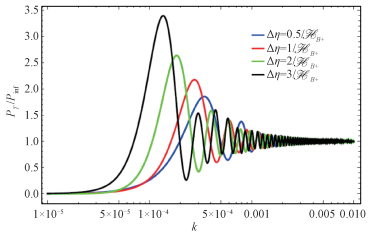
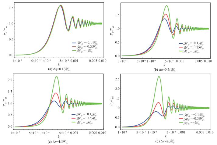
Figure 2 shows the spectra with different bounce durations. Considering that the bounce no longer contains symmetry in broad bounce, we plot Fig. 3, in which the first wave crest of spectrum is depressed with the increasing of asymmetry of bounce shape at a determined bounce duration, and this feature turns more obvious in broad bounce.
Fig. 2
 | Download: JPG larger image |
Fig. 2 | |
Fig. 3
 | Download: JPG larger image |
Fig. 3 Power spectra with different bounce times | |
Figures 4(a), 4(b), and 4(c) show the differences between the narrow and broad bounces. The curve of the second order turns to be abnormal when bounce turns to be broad. Though the bounce inflation has not been verified by experiment, some fitting studies have been carried out, such as Ref.[25]. If we detect the power spectrum in such a shape in future, we can accurately check the theory and distinguish between the broad bounce and the narrow bounce.
Fig. 4
 | Download: JPG larger image |
Fig. 4 Contrast between narrow bounce and broad bounce | |
The first order for narrow bounce, and the second order for broad bounce.
3 DiscussionThe bounce inflation is successful in solving the initial singularity problem of inflation and is also competitive in explaining the power deficit in CMB at large scale. This might provide a chance to comprehend the origin of inflation thoroughly. Theoretically, previous work successfully deals with the case with the narrow bounce. It is not only for a much extensive prediction, but also for the completion of the theory. We naturally generalize the narrow bounce to the broad bounce. In this study, we calculate the tensor perturbation in the bounce inflation scenario with the broad bounce. We get the result in a more precise approximation, and compare our result with that in narrow bounce model.
References
| [1] | Guth A H. Inflationary universe:a possible solution to the horizon and flatness problems[J]. Physical Review D, 1981, 23(2): 347-356. |
| [2] | Linde A D. A new inflationary universe scenario:a possible solution of the horizon, flatness, homogeneity, isotropy and primordial monopole problems[J]. Physics Letters B, 1982, 108(6): 389-393. DOI:10.1016/0370-2693(82)91219-9 |
| [3] | Albrecht A, Steinhardt P J. Cosmology for grand unified theories with radiatively induced symmetry breaking[J]. Physical Review Letters, 1982, 48(17): 1220-1223. DOI:10.1103/PhysRevLett.48.1220 |
| [4] | Komatsu E, Smith K M, Dunkley J, et al. Seven-year wilkinson microwave anisotropy probe (WMAP) observations: cosmological interpretation[C]//Intelligent Signal Processing and Communication Systems (ISPACS), 2010 International Symposium on. IEEE, 2010: 1-4. |
| [5] | Piao Y S, Feng B, Zhang X. Suppressing the CMB quadrupole with a bounce from the contracting phase to inflation[J]. Physical Review D, 2013, 88(6): 90-103. |
| [6] | Piao Y S. Possible explanation to a low CMB quadrupole[J]. Physical Review D, 2005, 71(8): 287-294. |
| [7] | Piao Y S, Tsujikawa S, Zhang X. Inflation in string-inspired cosmology and suppression of CMB low multipoles[J]. Classical & Quantum Gravity, 2003, 21(18): 4455-4461. |
| [8] | Biswas T, Mazumdar A. Super-inflation, non-singular bounce, and low multipoles[J]. Classical & Quantum Gravity, 2013, 31(2): 25019-25025. |
| [9] | Liu Z G, Guo Z K, Piao Y S. Obtaining the CMB anomalies with a bounce from the contracting phase to inflation[J]. Physical Review D, 2013, 88(6): 063539. DOI:10.1103/PhysRevD.88.063539 |
| [10] | Liu Z G, Guo Z K, Piao Y S. CMB anomalies from an inflationary model in string theory[J]. European Physical Journal C, 2014, 74(8): 3006. DOI:10.1140/epjc/s10052-014-3006-0 |
| [11] | Falciano F T. Classical bounce:constraints and consequences[J]. Physical Review D, 2012, 77(8): 284-299. |
| [12] | Lilley M, Lorenz L, Clesse S. Observational signatures of a non-singular bouncing cosmology[J]. Journal of Cosmology & Astroparticle Physics, 2011, 6(6): 1167-1183. |
| [13] | Mielczarek J. Gravitational waves from the big bounce[J]. Journal of Cosmology & Astroparticle Physics, 2008, 2008(11): 458-461. |
| [14] | Xia J Q, Cai Y F, Li H, et al. Evidence for bouncing evolution before inflation after BICEP2[J]. Physical Review Letters, 2014, 112(25): 251301. DOI:10.1103/PhysRevLett.112.251301 |
| [15] | Wang Y T, Piao Y S. Parity violation in pre-inflationary bounce[J]. Physics Letters B, 2015, 741(C): 55-60. |
| [16] | Qiu T, Wang Y T. G-bounce inflation:towards nonsingular inflation cosmology with galileon field[J]. Journal of High Energy Physics, 2015, 4(4): 1-28. |
| [17] | Wan Y, Qiu T, Huang F P, et al. Bounce inflation cosmology with standard model higgs boson[J]. Journal of Cosmology & Astroparticle Physics, 2015(12): 19. |
| [18] | Cai Y, Wan Y, Li H G, et al. The effective field theory of nonsingular cosmology[J]. Journal of High Energy Physics, 2017(1): 90. |
| [19] | Cai Y, Li H G, Qiu T, Piao Y S. The effective field theory of nonsingular cosmology:Ⅱ[J]. The European Physical Journal C, 2017, 77(6): 369. DOI:10.1140/epjc/s10052-017-4938-y |
| [20] | Cai Y, Piao Y S. A covariant Lagrangian for stable nonsingular bounce[J]. Journal of High Energy Physics, 2017, 2017(9): 27. DOI:10.1007/JHEP09(2017)027 |
| [21] | Cai Y, Wang Y T, Piao Y S. Pre-inflationary primordial perturbations[J]. Phys Rev D, 2015, 92. |
| [22] | Battefeld D, Peter P. A critical review of classical bouncing cosmologies[J]. Physics Reports, 2014, 571: 1-66. |
| [23] | Lehners J L. Cosmic bounces and cyclic universes[J]. Classical & Quantum Gravity, 2011, 28(20): 3990-3997. |
| [24] | Guzzetti M C, Bartolo N, Liguori M, et al. Gravitational waves from inflation[J]. Nuovo Cimento Rivista Serie, 2016, 39: 399-495. |
| [25] | Li H G, Cai Y, Piao Y S. Towards the bounce inflationary gravitational wave[J]. European Physical Journal C, 2016, 76(12): 699. DOI:10.1140/epjc/s10052-016-4554-2 |
