Yong Wang1,2,Rongzheng Zhang1,2
(1.Research Institute of Electronic Engineering Technology, Harbin Institute of Technology, Harbin 150001, China; 2. Key Laboratory of Marine Environmental Monitoring and Information Processing, Ministry of Industry and Information Technology, Harbin 150001, China)
Abstract:
High-resolution of Inverse Synthetic Aperture Radar (ISAR) in the azimuth direction can be achieved by increasing the coherent accumulation angle of the target rotation. However, in practice, the coherent accumulation angle may be small. In this paper, a novel algorithm for high-resolution ISAR imaging based on the SParse Iterative Covariance-based Estimation (SPICE) is proposed. As a nonparametric sparse spectrum estimation algorithm, the SPICE algorithm does not need to set any parameters and it converges globally, so it can realize high quality imaging with limited measurements. In addition, a fast implementation of the SPICE algorithm based on the Gohberg-Semencul (G-S) factorization is introduced in this paper. The ISAR imaging of simulated and measured data was analyzed to illustrate the effectiveness of the novel approach.
Key words: ISAR high-resolution SPICE fast implementation
DOI:10.11916/j.issn.1005-9113.18109
Clc Number:TN957.51
Fund:
Yong Wang, Rongzheng Zhang. High-Resolution ISAR Imaging Based on Sparse Iterative Covariance-Based Estimation[J]. Journal of Harbin Institute of Technology (New Series), 2019, 26(3): 1-6. DOI: 10.11916/j.issn.1005-9113.18109.

Fund Sponsored by the National Natural Science Foundation of China(Grant Nos. 61622107 and 61871146) Corresponding author Winner of the National Science Fund for Excellent Youth Scholars and the Program for New Century Excellent Talents in University of Ministry of Education. Yong Wang, E-mail: wangyong6012@hit.edu.cn Article history Received: 2018-09-10
Contents Abstract Full text Figures/Tables PDF
High-Resolution ISAR Imaging Based on Sparse Iterative Covariance-Based Estimation
Yong Wang1,2

 , Rongzheng Zhang1,2
 1. Research Institute of Electronic Engineering Technology, Harbin Institute of Technology, Harbin 150001, China;
2. Key Laboratory of Marine Environmental Monitoring and Information Processing, Ministry of Industry and Information Technology, Harbin 150001, China
Received: 2018-09-10
Fund: Sponsored by the National Natural Science Foundation of China(Grant Nos. 61622107 and 61871146)
Corresponding author: Winner of the National Science Fund for Excellent Youth Scholars and the Program for New Century Excellent Talents in University of Ministry of Education. Yong Wang, E-mail: wangyong6012@hit.edu.cn
Abstract: High-resolution of Inverse Synthetic Aperture Radar (ISAR) in the azimuth direction can be achieved by increasing the coherent accumulation angle of the target rotation. However, in practice, the coherent accumulation angle may be small. In this paper, a novel algorithm for high-resolution ISAR imaging based on the SParse Iterative Covariance-based Estimation (SPICE) is proposed. As a nonparametric sparse spectrum estimation algorithm, the SPICE algorithm does not need to set any parameters and it converges globally, so it can realize high quality imaging with limited measurements. In addition, a fast implementation of the SPICE algorithm based on the Gohberg-Semencul (G-S) factorization is introduced in this paper. The ISAR imaging of simulated and measured data was analyzed to illustrate the effectiveness of the novel approach.
Keywords: ISAR high-resolution SPICE fast implementation
1 Introduction ISAR imaging system obtains the high range resolution by transmitting wideband signals and the azimuth resolution by the coherent accumulation of the target echo to achieve a Range-Doppler image. Due to the fact that the actual system may have a limited number of echoes or some of the echoes are subject to strong interference, the resolution of the traditional FFT-based Range-Doppler algorithm may not be able to meet the requirements. When the coherent accumulation angle is limited, it is necessary to use the super-resolution method for ISAR imaging[1-2].
At present, most common ISAR super-resolution imaging methods are mainly classified into the nonparametric spectral estimation[3-5] and the Compressive Sensing (CS)[6-8]. The nonparametric spectrum estimation has a wide range of applications because no parameter needs to be set, while its resolution improvement is limited and the calculation is cumbersome. The CS algorithm exploits the sparseness of the echo at the scattering point, which makes a breakthrough to the Nyquist sampling theorem and can obtain a higher resolution. However, the use of the algorithm needs to predict the sparsity level of the signal and may lose part of the information.
In this paper, a nonparametric sparse spectrum estimation algorithm for ISAR imaging based on SPICE[9-11] is proposed. The algorithm uses the sparseness of the signal without setting any parameters, which can effectively improve the resolution of ISAR imaging. In order to reduce the amount of calculation, this paper also introduces a fast implementation of the SPICE algorithm based on the G-S factorization[12-13]. The ISAR imaging of simulated and measured data can illustrate the effectiveness of the SPICE algorithm.
The structure of this paper is as follows. The ISAR imaging principle is introduced in Section 2. Section 3 presents the principle of SPICE and the fast implementation of the SPICE algorithm is described in Section 4. The imaging results are discussed in Section 5 with the conclusions drawn in Section 6.
2 Signal Model The general situation of ISAR imaging is that the radar does not move while the target moves. To simplify the model, as shown in Fig. 1, we assumed that the translational component of the target motion has been compensated, leaving only the rotational component.
Fig.1
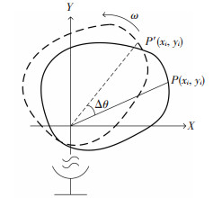 Fig.1 The turntable imaging geometry
 It is assumed that during the observation process, the target turns a small angle against the reference point. At a slow time, the signal in each range cell can be expressed as
$\begin{array}{*{20}{c}}{y\left( {{t_m}} \right) = \sum\limits_{i = 1}^K {{\sigma _i}} \exp \{ \frac{{ - {\rm{j}}4\pi }}{\lambda }\left[ {{x_i}\sin \left( {\omega {t_m}} \right) + } \right.}\\{{y_i}\left( {1 - \cos \left( {\omega {t_m}} \right)} \right)]\} }\end{array}$ (1)
where λ denotes the wavelength, ω is the angular velocity of rotation, σi denotes the magnitude of the scattering point, and (xi, yi) denotes the position of the scattering point. If tm is small, then sin(ωtm)≈ω tm and cos(ω tm)≈1. Therefore, the signal within each range cell can be represented as single frequency signals as follows:
$y\left( {{t_m}} \right) = \sum\limits_{i = 1}^K {{\sigma _i}} \exp \left( {\frac{{ - {\rm{j}}4\pi {x_i}\omega {t_m}}}{\lambda }} \right)$ (2)
In practice, there are only a few effective scattering points in a range cell, so the SPICE algorithm can be used to improve the resolution.
3 SPICE Algorithm Let K denote the number of sampling points in the frequency domain. If y =[y(t1), …, y(tN)]T denotes a time domain signal of length N, ak=[exp(j ωk t1), …, exp(j ωk tN)]T denotes a Fourier vector at ωk, then we can rewrite formula (2) in the sparse form as follows:
$\boldsymbol{y}=\sum\limits_{k=1}^{K} s_{k} \boldsymbol{a}_{k}+{\varepsilon}=\left[\boldsymbol{a}_{1}, \cdots, \boldsymbol{a}_{K}, \boldsymbol{I}\right]\left[\begin{array}{l}{\boldsymbol{s}} \\ {\boldsymbol{\varepsilon}}\end{array}\right]=\boldsymbol{A} \boldsymbol{\beta}$ (3)
where
$\begin{array}{l}{\boldsymbol{s}=\left[s_{1}, \cdots, s_{k}\right]^{\mathrm{T}}, \boldsymbol{\beta}=\left[\boldsymbol{s}^{\mathrm{T}}, \boldsymbol{\varepsilon}^{\mathrm{T}}\right]^{\mathrm{T}}} \\ {\boldsymbol{A}=\left[\boldsymbol{a}_{1}, \cdots, \boldsymbol{a}_{K}, \boldsymbol{I}\right]=\left[\boldsymbol{a}_{1}, \cdots, \boldsymbol{a}_{K+N}\right]}\end{array}$ (4)
where ε denotes noise term, {sk}k=1K denotes the corresponding amplitude at ωk. Since y is a sparse signal, most of the elements in {sk}k=1K are zero. If the noise covariance matrix is expressed as diag{σ1, σ2, …, σN}, the covariance matrix of the signal can be expressed as
$ \boldsymbol{R}= E\left(\boldsymbol{y} \boldsymbol{y}^{\mathrm{H}}\right)=\sum\limits_{k=1}^{K}\left|s_{k}\right|^{2} \boldsymbol{a}_{k} \boldsymbol{a}_{k}^{\mathrm{H}}+\\ \operatorname{diag}\left\{\sigma_{1}, \sigma_{2}, \right., \cdots, \sigma_{N} \} \triangleq \boldsymbol{A} \boldsymbol{P} \boldsymbol{A}^{\mathrm{H}} $ (5)
where H represents the conjugate transpose and
$\begin{aligned} \boldsymbol{P}=& \operatorname{diag}\left\{\left|s_{1}\right|^{2}, \cdots, \left|s_{K}\right|^{2}, \sigma_{1}, \cdots, \sigma_{N}\right\}=\\ & \operatorname{diag}\left\{p_{1}, \cdots, p_{N+K}\right\} \end{aligned}$ (6)
Using the covariance fitting criterion, the following optimization problem is obtained
$f=\left\|\boldsymbol{R}^{-1 / 2}\left(\boldsymbol{y} \boldsymbol{y}^{\mathrm{H}}-\boldsymbol{R}\right)\right\|^{2}$ (7)
where ‖·‖ represents the Frobenius norm of the matrix, and R-1/2 is the square root of the Hermitian positive definite matrix R-1. After a calculation[4], it can be deduced that the minimization of f is the same as that of the following problem
$\mathop {\min }\limits_p {\mathit{\boldsymbol{y}}^{\rm{H}}}{\mathit{\boldsymbol{R}}^{ - 1}}\mathit{\boldsymbol{y}} + \sum\limits_{k = 1}^{K + N} {w_k^2} {p_k};{w_k} = \frac{{\left\| {{\mathit{\boldsymbol{a}}_k}} \right\|}}{{\left\| \mathit{\boldsymbol{y}} \right\|}}$ (8)
For the convenience of calculation, Eq. (8) is changed to the following constraint minimization problem
$\begin{aligned} \min\limits_{p, \beta} \boldsymbol{\beta}^{\mathrm{H}} \boldsymbol{P}^{-1} \boldsymbol{\beta} &+\sum\limits_{k=1}^{K+N} w_{k}^{2} p_{k} \\ \text { s.t } \boldsymbol{A} \boldsymbol{\beta} &=\boldsymbol{y} \end{aligned}$ (9)
During the iteration, we can fix P to calculate the update of β, and the results can be obtained from Ref. [4] as follows:
$\boldsymbol{\beta}=\boldsymbol{P} \boldsymbol{A}^{\mathrm{H}} \boldsymbol{R}^{-1} \boldsymbol{y}$ (10)
After completing the update of β, P needs to be calculated by using formula (9). Since the scattering points of the target are independent from each other, the minimum update of each frequency point can be calculated separately. So Eq.(9) can be reduced to the following form
$\min\limits_{p \geqslant 0} \frac{|\beta|^{2}}{p}+w^{2} p$ (11)
The optimal solution is
$p_{k}=\frac{\left|\beta_{k}\right|^{2}}{w_{k}}, k=1, 2, \cdots, K+N$ (12)
It can be seen from the above analysis that, through iterative operations, the values of {pk}k=1K+N and β are updated alternately so that the algorithm runs stably. According to Ref. [9], for any initial value {pk≥0}, the results of the iteration will converge to the optimal solution. However, the initialization of pk=|ak* y |2/‖ak‖4(k=1, 2, …, K+N) by the single-frequency least-squares (SFLS) method can accelerate the convergence speed.
4 Fast Implementation of SPICE The iteration of SPICE needs the calculation of the inverse of the covariance matrix R-1 in Eq.(10), and the computational cost of computing R-1 is O(N3). Since the running time of the SPICE algorithm is dominated by calculating the inverse of the covariance matrix, a method is introduced in this section for the fast calculation of R-1 in the SPICE algorithm. R is rewritten as
$\boldsymbol{R}_{N}=\sum\limits_{k=1}^{K}\left|s_{k}\right|^{2} \boldsymbol{a}_{k} \boldsymbol{a}_{k}^{*}+\operatorname{diag}\left\{\sigma_{1}, \sigma_{2}, \cdots, \sigma_{N}\right\}=\\\left[\begin{array}{cccc}{r_{0}+\sigma_{1}} & {r_{1}} & {\cdots} & {r_{N-1}} \\ {r_{1}^{*}} & {r_{0}+\sigma_{2}} & {\cdots} & {r_{N-2}} \\ {\vdots} & {\vdots} & {\ddots} & {\vdots} \\ {r_{N-1}^{*}} & {r_{N-2}^{*}} & {\cdots} & {r_{0}+\sigma_{N}}\end{array}\right]$ (13)
Suppose that the noise variance is constant throughout the slow time, i.e., σ1=…=σN=σ. RN becomes a Toeplitz and Hermitian matrix, so we can use the method in Refs. [6-7] to perform G-S factorization to reduce the amount of computation for inversion. First, RN is expressed as
$\boldsymbol{R}_{N}=\left[\begin{array}{cc}{r_{0}+\sigma} & {\boldsymbol{r}_{N-1}^{\mathrm{H}}} \\ {\boldsymbol{r}_{N-1}} & {\boldsymbol{R}_{N-1}}\end{array}\right]=\left[\begin{array}{cc}{\boldsymbol{R}_{N-1}} & {\hat{\boldsymbol{r}}_{N-1}^{*}} \\ {\hat{\boldsymbol{r}}_{N-1}^{\mathrm{T}}} & {r_{0}+\boldsymbol{\sigma}}\end{array}\right]$ (14)
where rN-1=[r1*, r2*, …, rN-1*]T and
$\boldsymbol{w}_{N-1}=-\boldsymbol{R}_{M-1}^{-1} \boldsymbol{r}_{M-1}$ (15)
$\alpha_{N-1}=r_{0}+\sigma-\boldsymbol{r}_{N-1}^{\mathrm{H}} \boldsymbol{R}_{N-1}^{-1} \boldsymbol{r}_{N-1}$ (16)
Let LN(t, Z)=[t, Zt, …, ZN-1t]. ZN denotes an M × M strictly lower-triangular matrix with ones on the first sub-diagonal and zeros everywhere else. So we can use G-S factorization to write R-1 as
$\boldsymbol{R}_{N}^{-1}=L_{N}\left(\boldsymbol{t}_{1}, \boldsymbol{Z}_{N}\right) L_{N}^{\mathrm{H}}\left(\boldsymbol{t}_{1}, \boldsymbol{Z}_{N}\right)-L_{N}\left(\boldsymbol{t}_{2}, \boldsymbol{Z}_{N}\right) L_{W}^{\mathrm{H}}\left(\boldsymbol{t}_{2}, \boldsymbol{Z}_{N}\right)$ (17)
where
$\begin{aligned} \boldsymbol{t}_{1} &=\frac{1}{\sqrt{\alpha_{M-1}}}\left[1, \boldsymbol{w}_{M-1}\right]^{\mathrm{T}} \\ \boldsymbol{t}_{2} &=\frac{1}{\sqrt{\alpha_{M-1}}}\left[0, \hat{\boldsymbol{w}}_{M-1}^{*}\right]^{\mathrm{T}} \end{aligned}$ (18)
From the above analysis, it can be seen that only wN-1 and αN-1 are needed to get R-1, and the calculation of wN-1 and αN-1 by the Levinson-Durbin algorithm[12, 14] requires only N2 operations. In Eq.(17), both LN(t1, ZN) and LN(t2, ZN) are triangular Toeplitz matrices, so the FFT can be used to calculate R-1y in Eq.(10)[14]. Compared with the direct calculation of R-1, the proposed method greatly reduces the amount of computation for each iteration.
The fast implementation ofthe SPICE algorithm can be summarized as follows:
Initialization:
Calculate {pk}k=1K+N using SFLS and calculate wk in Eq.(8).
The (i+1)th iteration:
1) Construct the covariance matrix R in Eq.(5) using FFT with O(Klog2K) flops[13];
2) Calculate wN-1 and αN-1 using the Levinson-Durbin (L-D)-type algorithm with O(N2) flops;
3) Calculate R-1y using FFT with O(N2log2N) flops, calculate β by Eq.(10), and then update {pk}k=1K+N by Eq.(12) with O(N2K) flops;
4) Stop the iterative operation according to the predetermined threshold.
5 Experiments and Discussion To verify the proposed method, we simulated a multi-component sinusoidal signal. The amplitude and frequency of the four components are (0.5, 1.46 Hz), (1.0, 2.34 Hz), (1.5, 3.26 Hz), and (1.5, 3.46 Hz). SPICE algorithm was used for spectral estimation of this signal. The number of sampling points is 128. Fig. 2 shows the relationship between the energy difference and the number of iterations for adjacent iterations of the SPICE algorithm.
Fig.2
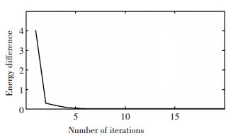 Fig.2 Relation between the energy difference and the number of iterations of SPICE
 In practical applications, we can assume that the iteration converges when the energy difference is less than one percent of the total energy and the number of iterations is usually less than ten. Fig. 3 (a) is the result of spectrum estimation by FFT, which indicates that if FFT is used directly, the resolution cannot meet the requirement due to the small number of sampling points. Fig. 3 (b) is the result of SPICE, which shows that the SPICE algorithm had lower sidelobes and is more accurate for the amplitude estimates than the FFT.
Fig.3
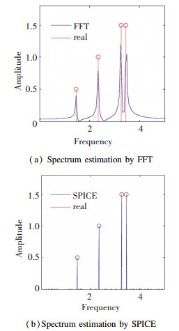 Fig.3 Results of spectrum estimation by FFT and SPICE
 Fig. 4 shows the flowchart for ISAR imaging using the SPICE algorithm. Motion compensation was performed on the high resolution range image, and the azimuth compression of the signal in each range cell was then performed using the improved SPICE algorithm proposed in this paper. In this experiment, the FFT, Iterative Adaptive Approach (IAA)[3, 15], and the SPICE algorithm were compared.
Fig.4
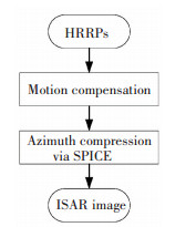 Fig.4 ISAR imaging using the SPICE algorithm
 The simulated MIG-25 data was used for the ISAR imaging experiment. The stepped-frequency radar works at 9 GHz and the pulse repetition frequency is 15 kHz. A total of 512 pulses, 64 samples were collected from each pulse. Figs. 5 (a)-(c) show the results of MIG-25 imaging by FFT, IAA, and the fast implementation of SPICE algorithm, respectively. It can be seen that both IAA and SPICE algorithm can improve the resolution of the image, while the SPICE algorithm works better than the IAA.
Fig.5
 Fig.5 Results of MIG-25 imaging by FFT, IAA, and the fast implementation of SPICE algorithm
 The entropy of the three images was calculated to compare their resolutions, whose results were 7.859 9, 7.272 5, and 6.549 6, respectively, which indicates that the ISAR image obtained by the SPICE algorithm has the best focus performance.
In order to verify the effectiveness of the SPICE in practice, the measured data from the Yak-42 plane was used. The radar transmits an LFM signal at a carrier frequency of 5 520 MHz with a bandwidth of 400 MHz. The pulse repetition frequency is 400 Hz. Here we only use 128 consecutive pulses. Fig. 6 (a) shows the result of Yak-42 imaging by FFT, which was blurry due to the short accumulation time. Fig. 6 (b) illustrates the result of IAA, which indicates that the IAA algorithm can improve the resolution of ISAR imaging. Fig. 6 (c) is the imaging result of the fast implementation of SPICE algorithm, which shows that the image quality was further improved.
Fig.6
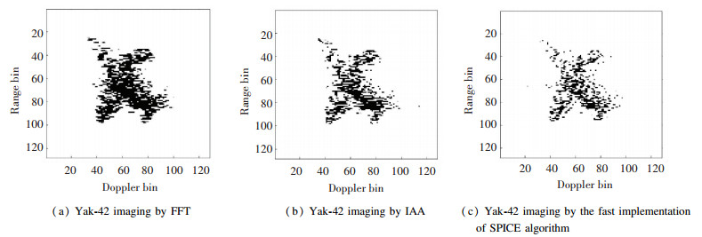 Fig.6 Results of Yak-42 imaging by FFT, IAA, and the fast implementation of SPICE algorithm
 The entropy of the three images was calculated, in which the image using FFT was 7.327 3, using IAA was 7.042 7, and using the fast implementation of SPICE algorithm was 6.613 1, among which the image resolution using the SPICE algorithm was the highest.
6 Conclusions In this paper, a novel high-resolution imaging algorithm based on SPICE is proposed to solve the problem of short accumulation time of ISAR imaging. The basic principles of ISAR imaging and SPICE algorithm were briefly described, and a fast implementation of the SPICE was introduced. The amount of calculation was reduced by G-S factorization and FFT. Experiments on simulated MIG-25 data and measured Yak-42 data show that the proposed algorithm can significantly improve the resolution of ISAR imaging.
References
[1] Bon N, Khenchaf A, Garello R. Airborne scan mode ISAR imagery of ships using high resolution spectral methods and particle filter. Proceedings of IGARSS 2004. 2004 IEEE International Geoscience and Remote Sensing Symposium. Piscataway: IEEE, 2004. 1506-1509. DOI: 10.1109/IGARSS.2004.1368707. (
 0)
0)[2] Mayhan J T, Burrows M L, Cuomo K M, et al. High resolution 3D "snapshot" ISAR imaging and feature extraction. IEEE Transactions on Aerospace and Electronic Systems, 2001, 37(2): 630-642. DOI:10.1109/7.937474 (
 0)
0)[3] Hu P, Xu S, Wu W, et al. IAA-based high-resolution ISAR imaging with small rotational angle. IEEE Geoscience and Remote Sensing Letters, 2017, 14(11): 1978-1982. DOI:10.1109/LGRS.2017.2744989 (
 0)
0)[4] Kalognomos G, Frangos P. Combining capon and APES noise covariance estimates for spectral estimation for ISAR applications. Proceedings of 2nd International Conference on Recent Advances in Space Technologies. Piscataway: IEEE, 2005. 694-698. DOI: 10.1109/RAST.2005.1512656. (
 0)
0)[5] Capon J. High-resolution frequency-wavenumber spectrum analysis. Proceedings of the IEEE, 1969, 57(8): 1408-1418. DOI:10.1109/PROC.1969.7278 (
 0)
0)[6] Wang Y, Kang J, Zhang R. ISAR imaging with random missing observations based on non-iterative signal reconstruction algorithm. Proceedings of 2014 12th International Conference on Signal Processing (ICSP). Piscataway: IEEE, 2014. 1876-1879. DOI: 10.1109/ICOSP.2014.7015318. (
 0)
0)[7] Ren X, Qiao L, Qin Y, et al. Sparse regularization based imaging method for inverse synthetic aperture radar. Proceedings of 2016 Progress in Electromagnetic Research Symposium (PIERS). Piscataway: IEEE, 2016. 4348-4351. DOI: 10.1109/PIERS.2016.7735622. (
 0)
0)[8] Qiu W, Zhao H, Zhou J, et al. High-resolution fully polarimetric ISAR imaging based on compressive sensing. IEEE Transactions on Geoscience and Remote Sensing, 2014, 52(10): 6119-6131. DOI:10.1109/TGRS.2013.2295162 (
 0)
0)[9] Stoica P, Babu P, Li J. New method of sparse parameter estimation in separable models and its use for spectral analysis of irregularly sampled data. IEEE Transactions on Signal Processing, 2011, 59(1): 35-47. DOI:10.1109/TSP.2010.2086452 (
 0)
0)[10] Stoica P, Babu P, Li J. SPICE: A SParse Covariance-based Estimation method for array processing. IEEE Transactions on Signal Processing, 2011, 59(2): 629-638. DOI:10.1109/TSP.2010.2090525 (
 0)
0)[11] Park H, Li J. A frequency-domain SPICE approach to high-resolution time delay estimation. IEEE Wireless Communications Letters, 2018, 7(3): 360-363. DOI:10.1109/LWC.2017.2778109 (
 0)
0)[12] Zhang Q, Abeida H, Xue M, et al. Fast implementation of SParse Iterative Covariance-based Estimation for array processing. Proceedings of 2011 Conference Record of the Forty Fifth Asilomar Conference on Signals, Systems and Computers (ASILOMAR). Piscataway: IEEE, 2011. 2031-2035. DOI: 10.1109/ACSSC.2011.6190383. (
 0)
0)[13] Xue M, Xu L, Li J. IAA spectral estimation: Fast implementation using the Gohberg-Semencul factorization. IEEE Transactions on Signal Processing, 2011, 59(7): 3251-3261. DOI:10.1109/TSP.2011.2131136 (
 0)
0)[14] Jain J. An efficient algorithm for a large Toeplitz set of linear equations. IEEE Transactions on Acoustics, Speech, and Signal Processing, 1979, 27(6): 612-615. DOI:10.1109/TASSP.1979.1163313 (
 0)
0)[15] Glentis G O, Jakobsson A. Efficient implementation of iterative adaptive approach spectral estimation techniques. IEEE Transactions on Signal Processing, 2011, 59(9): 4154-4167. DOI:10.1109/TSP.2011.2145376 (
 0)
0)