Rong Guo,Jimin Ye
(School of Mathematics and Statistics, Xidian University, Xi’an 710071, China)
Abstract:
Independent component analysis (ICA) can reveal the essential underlying structure of data, and independent component regression (ICR) methods usually obtain better performance than other regression methods such as principal component regression. However, when existing ICR methods separate or extract independent components using prewhitened data, the backward propagation of inevitable prewhitened errors deteriorates the final linear prediction accuracy. To overcome this weakness, first, we proposed using weighted orthogonal constraint condition to replace the prewhitening of the data in ICA. Next, the statistical independence of ICs and the close relationship between ICs and quality variables are considered at the same time. Then, by combining the merits of improved ICR and ensemble ICR algorithm which solved the problem of selecting an appropriate nonquadratic function in ICA iteration procedure, a modified independent component regression (MICR) method that directly used the measured process data was proposed. Finally, three experimental results were used to validate excellent performance of modified algorithm.
Key words: independent component analysis weighted orthogonal constraint independent component regression prewhitened data
DOI:10.11916/j.issn.1005-9113.17138
Clc Number:O212.4
Fund:
Rong Guo, Jimin Ye. Modified Independent Component Regression Method Without Prewhitening[J]. Journal of Harbin Institute of Technology (New Series), 2019, 26(4): 50-57. DOI: 10.11916/j.issn.1005-9113.17138.

Fund Sponsored by the National Natural Science Foundation of China (Grant No. 61573014) Corresponding author Jimin Ye, E-mail: jmye@mail.xidian.edu.cn Article history Received: 2017-11-14
Contents Abstract Full text Figures/Tables PDF
Modified Independent Component Regression Method Without Prewhitening
Rong Guo

 , Jimin Ye
 School of Mathematics and Statistics, Xidian University, Xi'an 710071, China
Received: 2017-11-14
Sponsored by the National Natural Science Foundation of China (Grant No. 61573014)
Corresponding author: Jimin Ye, E-mail: jmye@mail.xidian.edu.cn
Abstract: Independent component analysis (ICA) can reveal the essential underlying structure of data, and independent component regression (ICR) methods usually obtain better performance than other regression methods such as principal component regression. However, when existing ICR methods separate or extract independent components using prewhitened data, the backward propagation of inevitable prewhitened errors deteriorates the final linear prediction accuracy. To overcome this weakness, first, we proposed using weighted orthogonal constraint condition to replace the prewhitening of the data in ICA. Next, the statistical independence of ICs and the close relationship between ICs and quality variables are considered at the same time. Then, by combining the merits of improved ICR and ensemble ICR algorithm which solved the problem of selecting an appropriate nonquadratic function in ICA iteration procedure, a modified independent component regression (MICR) method that directly used the measured process data was proposed. Finally, three experimental results were used to validate excellent performance of modified algorithm.
Keywords: independent component analysis weighted orthogonal constraint independent component regression prewhitened data
1 Introduction In recent years, regression analyses had been applied more and more widely[1-3]. Common regression analysis includes: principal component regression (PCR), partial least squares regression (PLSR) and multiple linear regression (MLR). However, because of the high dimension and linear correlation between process variables and quality variable, it is hard to deal with data in MLR, and neither PCR nor PLSR will recover true latent variables. Additionally, PCR/PLSR can only tackle the first and second moment of data, ignoring higher moment. ICA can recover independent source signals from mixed signals. Independence was a condition that can reveal the essential underlying data structure and made full use of higher-order moments information[4-6].
Because of the advantages of ICA, ICR was developed for regression in recent years[6-9]. Although the conventional ICR model is meaningful for regression analysis, it still has some disadvantages. First, the random initialization of the demixing matrix can bring about different optimization solutions, which might generate uncertain model results. Second, there is no particular criterion to determine which nonquadratic function used in ICA algorithms is optimal. Third, even if the extracted ICs are independent of each other, they may not carry the information of the quality variable and do not contribute to predictions and interpretations. If we employ all separated ICs to interpret the quality variables, it will lead to complex modeling and overfitting easily in regression analysis. Lee and Qin[10] solved the first problem with modified ICA (MICA). MICA replaces the random initialization condition of the original ICA with fixing initialization condition to produce a specific ICA solution. With respect to the second weakness, the ensemble modified ICR (EMICR) method presented by Tong[11-12] built an ensemble model that combined the results of multiple regression models with three different nonquadratic functions. This integrated method possesses better performance than a single-model method. A dual-objective cost function is built by Zhao[13] to solve the third issue. Nevertheless, the above approaches apply a whitening procedure before separating the independent components.
Whitening procedures remove second-order dependence from data X and make it easier to solve the separation problem. Generally, the whitening error cannot be avoided and will reduce the accuracy of model. When some source signals are weak or the mixing matrix is ill-conditioned, this phenomenon will become more serious.
To overcome above issues, substituting the prewhitening step in ICA with weighted orthogonal constraint, combining the advantages of the improved ICR algorithm raised by Zhao[13] with those of the EMICR algorithm suggested by Tong[11], a modified independent component regression (MICR) method was put forward, which estimated the regression coefficients from measure data directly, and had better performance.
2 Theory 2.1 ICR Method Based on Prewhitened Data 2.1.1 Conventional ICR method ICR is the combination of an ICA model and regression analysis. Suppose that x=[x1, x2, …, xm]T represents the mixed variables. Assume that these variables are mixtures of some underlying latent variables s=[s1, s2, …, sd]T, namely, x=As, A∈Rm×d is mixing matrix, and that latent variables are mutually statistically independent, thus revealing the essential structure of the data. The idea of ICA is using observation variables x to estimate independent components vector[14]s and mixed matrix A. That is to find a separation matrix W and ?=Wx is the prediction of s. Before separating the independent components, the observation variable x is usually prewhitened. Prewhitened variable z=[z1, …, zd]T can be computed as below:
$\mathit{\boldsymbol{z}} = \mathit{\boldsymbol{Vx}}$ (1)
where V is the whitening matrix. The relationship between these variables is given by:
$\mathit{\boldsymbol{z}} = \mathit{\boldsymbol{VAs}} + \mathit{\boldsymbol{e}}$ (2)
where e∈Rd×1 is the residual vector. Using ICA, the separation matrix W is calculated, and the estimation of latent variable vector ? is obtained:
$\mathit{\boldsymbol{\hat s}} = \mathit{\boldsymbol{Wz}}$ (3)
Then, use the reconstructed latent variables ?1, ?2, …, ?d as the process variables for building a regression model:
$\left( {\begin{array}{*{20}{c}}{{y_1}}\\{{y_2}}\\ \vdots \\{{y_n}}\end{array}} \right) = \left( {\begin{array}{*{20}{c}}1&{{{\hat s}_{11}}}&{{{\hat s}_{12}}}& \cdots &{{{\hat s}_{1d}}}\\1&{{{\hat s}_{21}}}&{{{\hat s}_{22}}}& \cdots &{{{\hat s}_{2d}}}\\ \vdots & \vdots & \vdots & \vdots & \vdots \\1&{{{\hat s}_{n1}}}&{{{\hat s}_{22}}}& \cdots &{{{\hat s}_{nd}}}\end{array}} \right)\left( {\begin{array}{*{20}{c}}{{b_0}}\\{{b_1}}\\ \vdots \\{{b_d}}\end{array}} \right)$ (4)
${\rm{i}}{\rm{.e}}{\rm{.}}\;\mathit{\boldsymbol{y}} = \mathit{\boldsymbol{\hat Sb}}$ (5)
The regression coefficient can be obtained by the least square method as:
$\mathit{\boldsymbol{\hat b = }}{\left( {{{\mathit{\boldsymbol{\hat S}}}^{\rm{T}}}\mathit{\boldsymbol{\hat S}}} \right)^{ - 1}}{{\mathit{\boldsymbol{\hat S}}}^{\rm{T}}}\mathit{\boldsymbol{y}}$ (6)
Thus, estimation ? of regression coefficient h, which is directly related to mixed data X=[x1, x2, …, xn]T∈Rn×m, can be easily obtained from
$\mathit{\boldsymbol{y}} = \mathit{\boldsymbol{Z}}{\mathit{\boldsymbol{W}}^{\rm{T}}}\mathit{\boldsymbol{\hat b}} = \mathit{\boldsymbol{X}}{\mathit{\boldsymbol{V}}^{\rm{T}}}{\mathit{\boldsymbol{W}}^{\rm{T}}}\mathit{\boldsymbol{\hat b}} = \mathit{\boldsymbol{X}}{(\mathit{\boldsymbol{WV}})^{\rm{T}}}\mathit{\boldsymbol{\hat b}} = \mathit{\boldsymbol{X\hat h}}$ (7)
where
2.1.2 Ensemble modified ICR method In EMICR method, the cost function is based on the following approximation of negentropy [5]:
$J = {(E\{ G(y)\} - E\{ G(v)\} )^2}$ (8)
where v~N(0, 1), the EMICR model aims to build three ICR models base on three different nonquadratic functions instead employs a single ICR model, Hyv?rinen et al.[5] suggested three nonquadratic functions listed as follows:
$\left\{ {\begin{array}{*{20}{l}}{{G_1}(y) = \left( {1/{a_1}} \right)\log \cosh \left( {{a_1}y} \right)}\\{{G_2}(y) = \exp \left( { - {a_2}{y^2}/2} \right)}\\{{G_3}(y) = {y^4}}\end{array}} \right.$ (9)
Here, a1, a2∈[1,2], and generally, a1=a2=1. These equations are then combined into a single model. That is, we use the three different nonquadratic functions in Eq.(9) to build three different ICA models, and denote the three reconstructed latent variables as ?i,
${{\mathit{\boldsymbol{\hat s}}}_i} = {\mathit{\boldsymbol{W}}_i}\mathit{\boldsymbol{z}}$ (10)
where i=1, 2, 3, and the regression coefficient (according to the ith reconstructed latent variables) is:
${{\mathit{\boldsymbol{\hat b}}}_i} = {\left( {\mathit{\boldsymbol{\hat S}}_i^{\rm{T}}{{\mathit{\boldsymbol{\hat S}}}_i}} \right)^{ - 1}}\mathit{\boldsymbol{\hat S}}_i^{\rm{T}}\mathit{\boldsymbol{y}}$ (11)
${{\mathit{\boldsymbol{\hat h}}}_i} = {(\mathit{\boldsymbol{WV}})^{\rm{T}}}{{\mathit{\boldsymbol{\hat b}}}_i}$ (12)
Therefore, from Eqs.(7), (11) and (12), the prediction of quality variable y is:
${{\hat y}_i} = {\mathit{\boldsymbol{x}}^{\rm{T}}}{{\mathit{\boldsymbol{\hat h}}}_i}$ (13)
Then, combine the three regression formulas as a whole,
${\hat y_{{\rm{new}}}} = \sum\limits_{i = 1}^3 {{g_i}{{\hat y}_i}} $ (14)
where gi is obtained by optimizing the following Eq. (15):
$Q = \min \left\| {\mathit{\boldsymbol{y}} - \sum\limits_{i = 1}^3 {{g_i}{{\mathit{\boldsymbol{\hat y}}}_i}} } \right\|$ (15)
where y∈R1×n is the quality variable data vector and ? is the prediction of y.
Note that all of the existing ICR methods use data whitening z to separate the latent variables s. Prewhitening process will lead to error accumulation, and may deteriorate prediction accuracy, particularly when an online whitening process is used.
2.2 Modified ICR Method Based on Measured Data In both conventional ICRs and ensemble modified ICRs, latent variables are separated or extracted from prewhitened process variables. It is well known that prewhitening will introduce errors, and the backward propagation of those errors will reduce the prediction accuracy.
Replacing the prewhitening process with weighted orthogonal constraint condition on the separating matrix or extracting vectors, the latent variables can be directly separated or extracted from the measured process data[15], the error propagation is avoid. Additionally, in order to make the latent variables meaningful with respect to the quality variables, negentropy and the covariance between ICs and quality variables are simultaneously adopted for the iterative extraction of ICs. We propose the following dual-objective cost function based on measured process data:
$\begin{array}{l}J = \alpha \left\{ {E{{\left( {{\mathit{\boldsymbol{w}}^{\rm{T}}}\mathit{\boldsymbol{xy}}} \right)}^{\rm{T}}}E\left( {{\mathit{\boldsymbol{w}}^{\rm{T}}}\mathit{\boldsymbol{xy}}} \right)} \right\} + \\\;\;\;\;\;\;\;\;\beta {\left\{ {E\left\{ {G\left( {{\mathit{\boldsymbol{w}}^{\rm{T}}}\mathit{\boldsymbol{x}}} \right)} \right\} - E\left\{ {G(v)} \right\}} \right\}^2}\end{array}$ (16)
where α and β are the weight coefficients of each sub-optimization, and are defined to satisfy α+β=1.G is a nonquadratic function defined by Eq.(9). Because ICs are extracted individually, the weighted orthogonal constraint on extracting vectors
$\mathit{\boldsymbol{w}}_i^{\rm{T}}{\mathit{\boldsymbol{R}}_x}{\mathit{\boldsymbol{w}}_j} = {\delta _{i,j}}$ (17)
is used. Where wi denotes the extraction vector of the ith ICs. Simple calculation yields the gradient and Hessian matrix of J with respect to w
$\begin{array}{l}\nabla {J_w} = 2\alpha \mathit{\boldsymbol{R}}_x^{ - 1}E\left( {\mathit{\boldsymbol{x}}{\mathit{\boldsymbol{y}}^{\rm{T}}}} \right)E\left( {{\mathit{\boldsymbol{w}}^{\rm{T}}}\mathit{\boldsymbol{xy}}} \right) + \\\;\;\;\;\;\;\;2\beta \left( {E\left\{ {G\left( {{\mathit{\boldsymbol{w}}^{\rm{T}}}\mathit{\boldsymbol{x}}} \right)} \right\} - E\{ G(v)\} } \right) \cdot \\\;\;\;\;\;\;\;\;\mathit{\boldsymbol{R}}_x^{ - 1}E\left\{ {\mathit{\boldsymbol{x}}g\left( {{\mathit{\boldsymbol{w}}^{\rm{T}}}\mathit{\boldsymbol{x}}} \right)} \right\}\end{array}$ (18)
$\begin{array}{l}\frac{{{\partial ^2}J}}{{\partial {\mathit{\boldsymbol{w}}^2}}} = 2\alpha \mathit{\boldsymbol{R}}_x^{ - 1}\mathit{\boldsymbol{E}}\left( {\mathit{\boldsymbol{x}}{\mathit{\boldsymbol{y}}^{\rm{T}}}} \right)E\left( {\mathit{\boldsymbol{y}}{\mathit{\boldsymbol{x}}^{\rm{T}}}} \right) + \\\;\;\;\;\;\;\;2\beta \mathit{\boldsymbol{R}}_x^{ - 1}E\left\{ {\mathit{\boldsymbol{x}}g\left( {{\mathit{\boldsymbol{w}}^{\rm{T}}}\mathit{\boldsymbol{x}}} \right)} \right\}E{\left\{ {\mathit{\boldsymbol{x}}g\left( {{\mathit{\boldsymbol{w}}^{\rm{T}}}\mathit{\boldsymbol{x}}} \right)} \right\}^{\rm{T}}} + \\\;\;\;\;\;\;\;2\beta \left( {E\left\{ {G\left( {{\mathit{\boldsymbol{w}}^{\rm{T}}}\mathit{\boldsymbol{x}}} \right)} \right\} - E\{ G(v)\} } \right)E\left\{ {{g^\prime }\left( {{\mathit{\boldsymbol{w}}^{\rm{T}}}\mathit{\boldsymbol{x}}} \right)} \right\}\mathit{\boldsymbol{I}}\end{array}$ (19)
where g and g′ are respectively the first-order and second-order derivative of G. Using Newton's algorithm to solve the cost function (16), and applying a generalized Gram-Schmidt algorithm to implement the weighted orthogonal constraint on extracting vectors, the following iteration process is obtained:
$\Delta {\mathit{\boldsymbol{w}}_i} \propto {\left( {\frac{{{\partial ^2}J}}{{\partial \mathit{\boldsymbol{w}}_i^2}}} \right)^{ - 1}}\frac{{\partial J}}{{\partial {\mathit{\boldsymbol{w}}_i}}}$ (20)
${\mathit{\boldsymbol{w}}_i} = {\mathit{\boldsymbol{w}}_i} - \sum\limits_{j = 1}^{i - 1} {\left( {\mathit{\boldsymbol{w}}_i^{\bf{T}}{\mathit{\boldsymbol{R}}_x}{\mathit{\boldsymbol{w}}_j}} \right){\mathit{\boldsymbol{w}}_j}} $ (21)
${\mathit{\boldsymbol{w}}_i} = {\mathit{\boldsymbol{w}}_i}/\sqrt {\mathit{\boldsymbol{w}}_i^{\bf{T}}{\mathit{\boldsymbol{R}}_x}{\mathit{\boldsymbol{w}}_j}} $ (22)
Denoting W=[w1, …, wd]T then ?=XWT can be extracted directly from the observed data.And
$\mathit{\boldsymbol{y}} = \mathit{\boldsymbol{X}}{\mathit{\boldsymbol{W}}^{\rm{T}}}\mathit{\boldsymbol{\hat b}} = \mathit{\boldsymbol{X\hat h}}$ (23)
where
${\mathit{\boldsymbol{\hat S}}_i} = \mathit{\boldsymbol{XW}}_i^{\rm{T}}$ (24)
${\mathit{\boldsymbol{\hat b}}_i} = {\left( {\mathit{\boldsymbol{\hat S}}_i^{\rm{T}}{{\mathit{\boldsymbol{\hat S}}}_i}} \right)^{ - 1}}\mathit{\boldsymbol{\hat S}}_i^{\rm{T}}\mathit{\boldsymbol{y}}$ (25)
Thus,
Replacing prewhitening with weighted orthogonal constraint, error backward propagation is avoided. Using the covariance between ICs and quality variables, the extracted latent variables become meaningful to the quality variables. The solution produced by an ensemble approach is more effective and robust. We term the ICR method mentioned above as the modified ICR (MICR).
For the selection of optimized parameters α and β in Eq.(16), special criteria cannot be given easily which depend heavily on current practical applications. When prior knowledge is unavailable, the weight parameters can be determined by cross-validation and try and error method. If α>β, the correlation between ICs and quality variable is mainly considered. If α < β, the statistical independence of ICs is more important than the correlation between ICs and quality variable.Note, the prediction error is the most important factor in regression, generally, α is set bigger than β.
3 Experimental Results and Analysis In this chapter, we use three examples from different fields to verify the performance of the raised MICR approach. A rooted mean squared error (RMSE) index is employed to determine prediction accuracy:
${\rm{RMSE}} = \sqrt {\frac{{\sum\limits_{i = 1}^n {{{\left\| {\mathit{\boldsymbol{y}} - \mathit{\boldsymbol{\hat y}}} \right\|}^2}} }}{n}} $ (26)
where n is the number of test samples, ? and y are respectively predicted and real value vectors. Clearly, the smaller the RMSE value is, the higher the accuracy is.
3.1 Numerical Data Consider three source signals with the following distribution:
${s_1}(i) = 3\cos (0.02i)\sin (0.09i)$ (27)
${s_2}(i) = \sin (0.3i) + 2\cos (0.6i)$ (28)
${s_3}(i) = [ {\rm{rem}} (i,30) - 13]/9$ (29)
The rem function of Eq.(29) returns a remainder after division, while the mixing signals are generated by linear model x=As+e. The mixing matrix A is defined as:
$\mathit{\boldsymbol{A}} = \left( {\begin{array}{*{20}{r}}{0.67}&{0.79}&{0.86}\\{0.46}&{0.65}&{0.55}\\{ - 0.28}&{0.32}&{0.17}\\{0.27}&{0.12}&{- 0.33}\\{ - 0.89}&{ - 0.92}&{0.89}\\{0.76}&{0.74}&{0.35}\\{0.46}&{0.18}&{0.81}\\{0.02}&{0.41}&{0.01}\end{array}} \right)$ (30)
Noise e is a Gaussian variable of zero mean and standard deviation σ={0.1, 0.5, 1}. Setting y=3s1+s2+2s3, where y is the quality variable applied to regression analysis.The coefficients of s1, s2, and s3 can be randomly selected, and generally, the size of them are different, which means that the contribution of each IC to the quality variable is different. We can also employ two or one source signal to generate y. In MICR, the IC that does not contribute to the quality variable is extracted in the end, and will not be used as an explanatory variable. Even if it is used, from Eq. (25), we know that the estimated coefficient of it equals zero.
Choose one variance value (σ=0.1) of noise as an example. A total of 1 000 mixes are generated for model training, and 1 000 testing samples are generated for model prediction. A plot of the source signals can be seen in Fig. 1. Then, we use the numerical data to carry out the MICR method and conventional ICR with different G functions, and MICR method with EMICR method, using both measured and prewhitening data.
Fig.1
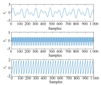 Fig.1 Source signals
 Note α should be bigger then β. Through try and error method we set α=0.7 and β=0.3. Fig. 2 and Fig. 3 describe the prediction results of the quality variable when selecting different number of ICs.
Fig.2
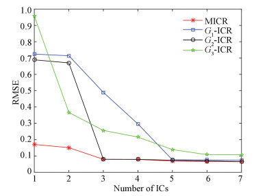 Fig.2 RMSE values vs. numbers of ICs (MICR and conventional ICR with different function G)
 Fig.3
 Fig.3 RMSE values vs. numbers of ICs(MICR and EMICR using whitening and measured data)
 Obviously, Fig. 2 and Fig. 3 illustrate that the MICR algorithm possesses better performance than conventional ICR and EMICR. It is easy to explain: in MICR, the error propagation is avoided because of dropping the prewhitening process, thus, the regression accuracy is improved, and MICR retains the merits of EMICR and improved ICR.
3.2 TE Process Data Tennessee Eastman (TE) process is a realistic industrial process[16] proposed by the Eastman Chemical Company. In the past few decades, the TE process has wide application in process control and detection[17-19]. The process is composed of a reactor, a condenser, a vapor-liquid separator, a recycle compressor, and a stripper, and measures 52 process variables in total. The process adopts 33 continuous variables with remaining 19 variables being composition measurements which are sampled less frequently. Table 1 lists some of the variables.
表 1
1Feed D
2Feed E
3Feed A
4Feed A and feed C
5Compressor cycle value
6Purge value
7Liquid flow of separator
8Stripper liquid flow value
9Stripper steam valve value
10Flow value of reactor cooling water
11Flow value of condenser cooling water
12Flow value of feed A
13Flow value of feed D
14Flow value of feed E
15Flow value of feed A and C
16Recycle flow
17Feed flow rate of reactor
18Reactor pressure
19Reactor level
20Reactor temperature
21Purge rate
22Separator temperature
23Separator level
24Separator pressure
25Separator bottom flow
26Stripper level
27Stripper pressure
28Stripper bottom flow
29Stripper temperature
30Upper steam flow of stripper
31Compressor power
32Outlet temperature of reactor cooling water
33Outlet temperature of separator cooling water
34A composition in purge
Table 1 Parts of variables for the TE process
In this case, the first 33 variables in Table 1 are the input variables and the last one is the output variable. We got the simulation datasets at http://web.mit.edu/braatzgroup/, and divided it into two parts: a training dataset contains 480 samples and a test dataset contains 960 samples. Suppose that the sampling intervals for input and output were 3 min and 6 min, respectively. The sub-optimization parameters were set to be α=0.8 and β=0.2. The selection of α and β is similar to the method used in chapter 2.2.
The quality prediction results (using the RMSE index) from the MICR algorithm can be seen in Fig. 4. Clearly, the proposed MICR algorithm yields a lower RMSE value than EMICR that uses prewhitening data and measured data. Additionally, only approximately 15 ICs require the use of regression analysis, successfully simplifying the model and improving system performance. The description of the actual value and the predicted value of the quality variable are shown in Fig. 5, which gives a visual impression of the quality variable and prediction. We can see that the predicted values are very close to the real values.
Fig.4
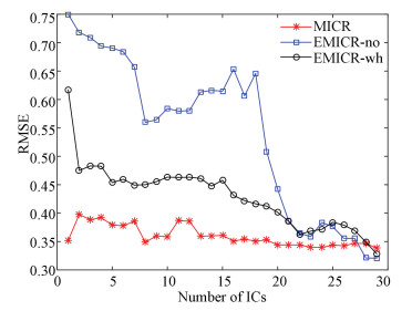 Fig.4 RMSE values vs. numbers of ICs(MICR and EMICR using whitening and measured data)
 Fig.5
 Fig.5 The comparison of quality variable and prediction
 3.3 Fetal Electrocardiogram Data (FECG) In present case study, to test the performance of the MICR method, we measured eight-channel cutaneous potential recordings on one pregnant woman's skin. Itis difficult to place an electrode directly on a baby because of several factors. Therefore, ECG recordings are usually measured on the mother's skin [20]. We download related data at the website: http://homes.esat.kuleuven.be/~smc/daisy/daisydata.html. Here, using the first 1500 samples as the training set, and an additional 1000 samples are used for evaluating the performance of model. Fig. 6 shows the potential test data recordings. In this example, recordings from channels 1 and 8 are used as quality variables y1 and y2 for regression analysis, and the signals from channels 2-7 are selected as the process variables x1-x6.
Fig.6
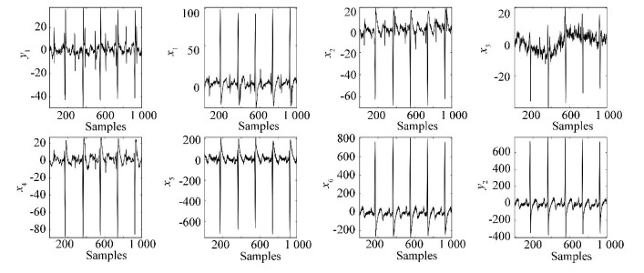 Fig.6 Recordings of FECG data
 Fig. 7 shows and compares the quality prediction results (using the RMSE index) from different algorithms in the case of whitening and non-whitening, respectively. The sub-optimization parameters are set as α=0.8 and β=0.2. They are calculated using 1000 samples and different numbers of ICs. The proposed MICR algorithm yields lower RMSE values than the EMICR algorithm using measured and prewhitening data. Additionally, only two ICs are needed to interpret variable y1 and one IC is needed to interpret variable y2. Thus, interpretation ability is improved and computational complexity is reduced. After model testing, we use different algorithms to calculate the RMSE values against different numbers of ICs and list final results in Table 2. In summary, the proposed MICR model predicts quality are more accurate than the EMICR model. Finally, the profiles of MICR method and conventional ICR with different functions G about quality variables y1 and y2 are given in Fig. 8. We can also see the advantages of ensemble learning in the ICR method.
Fig.7
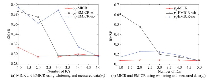 Fig.7 Description of RMSE values vs. numbers of ICs
 表 2
modelsOutput
variable1ICs2ICs3ICs4ICs5ICs
EMICR-whiteningy10.3850.3790.3100.3000.300
y20.6000.4800.2300.1800.140
EMICR-without
whiteningy10.3910.3600.3840.3190.291
y20.1800.2300.2100.2100.140
MICRy10.3280.2910.2890.3100.290
y20.1500.1400.1400.1300.130
Table 2 Results of the FECG dataset
Fig.8
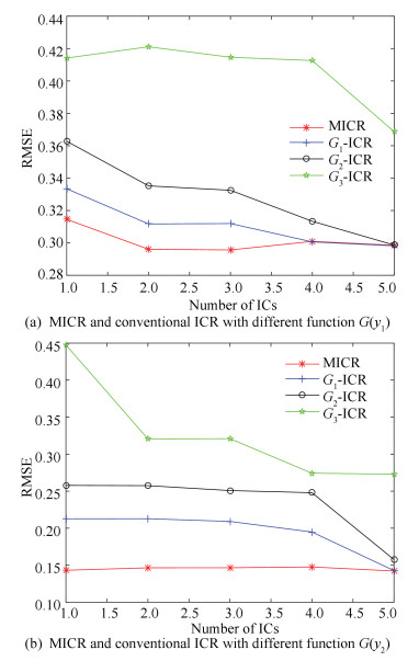 Fig.8 Description of RMSE values vs. numbers of ICs
 4 Conclusions The paper suggests an MICR method with non prewhitening process and considers the advantages of the EMICR and improved ICR algorithms. The proposed model is superior to the EMICR and improved ICR models because it uses three optimization objectives based on measured data in the IC extraction, which can separate more effective ICs. According to the experimental results, all simulations mentioned in this work have demonstrated that MICR method has effectiveness and better prediction performance than other methods.
While the present approach (without prewhitening) increases quality variable predictive capabilities and decreases data errors, the computational complexity of the model is sometimes high and holds promise for future research using the MICR algorithm.
References
[1] Rutledge R G, C?té C. Mathematics of quantitative kinetic PCR and the application of standard curves. Nucleic Acids Research, 2003, 31(16): e93. DOI:10.1093/nar/gng093 (
 0)
0)[2] Chung S J, Heymann H, Grün I U. Application of GPA and PLSR in correlating sensory and chemical data sets. Food Quality and Preference, 2003, 14(5-6): 485-495. DOI:10.1016/S0950-3293(03)00010-7 (
 0)
0)[3] Leone P A, Viscarra-Rossel R A, Amenta P, et al. Prediction of soil properties with PLSR and vis-NIR spectroscopy: Application to Mediterranean soils from southern Italy. Current Analytical Chemistry, 2012, 8(2): 283-299. DOI:10.2174/157341112800392571 (
 0)
0)[4] Pruim R H R, Mennes M, van Rooij D, et al. ICA-AROMA: A robust ICA-based strategy for removing motion artifacts from fMRI data. Neuroimage, 2015, 112: 267-277. DOI:10.1016/j.neuroimage.2015.02.064 (
 0)
0)[5] Hyv?rinen A, Oja E. Independent component analysis: Algorithms and applications. Neural Networks, 2000, 13(4-5): 411-430. DOI:10.1016/S0893-6080(00)00026-5 (
 0)
0)[6] Tong C, Palazoglu A, Yan X, et al. Improved ICA for process monitoring based on ensemble learning and Bayesian inference. Chemometrics & Intelligent Laboratory Systems, 2014, 135(14): 141-149. DOI:10.1016/j.chemolab.2014.04.012 (
 0)
0)[7] Kaneko H, Arakawa M, Funatsu A, et al. Development of a new regression analysis method using independent component analysis. Journal of Chemical Information & Modeling, 2008, 48(3): 534-541. DOI:10.1021/ci700245f (
 0)
0)[8] Westad F. Independent component analysis and regression applied on sensory data. Journal of Chemometrics banner, 2010, 19(3): 171-179. DOI:10.1002/cem.920 (
 0)
0)[9] Fan Liwei, Pan Sijia, Li Zimin, et al. An ICA-based support vector regression scheme for forecasting crude oil prices. Technological Forecasting & Social Change, 2016, 112: 245-253. DOI:10.1016/j.techfore.2016.04.027 (
 0)
0)[10] Lee J M, Qin S J, Lee I B. Fault detection and diagnosis based on modified independent component analysis. AiChE Journal, 2006, 52(10): 3501-3514. DOI:10.1002/aic.10978 (
 0)
0)[11] Tong Chudong, Lan Ting, Shi Xuhua. Soft sensing of non-Gaussian processes using ensemble modified independent component regression. Chemometrics & Intelligent Laboratory Systems, 2016, 157: 120-126. DOI:10.1016/j.chemolab.2016.07.006 (
 0)
0)[12] Tong Chudong, Lan Ting, Shi Xuhua. Double-layer ensemble monitoring of non-Gaussian processes using modified independent component analysis. ISA Transactions, 2017, 68: 181-188. DOI:10.1016/j.isatra.2017.02.003 (
 0)
0)[13] Zhao Chunhui, Gao Furong, Wang Fuli. An improved independent component regression modeling and quantitative calibration procedure. AiChE Journal, 2010, 56(6): 1519-1535. DOI:10.1002/aic.12079 (
 0)
0)[14] Hyv?rinen A, Hurri J, Hoyer P O. Independent Component Analysis. New Jersey: Wiley, 2001: 529-529. (
 0)
0)[15] Zhu Xiaolong, Zhang Xianda, Ding Zizhe, et al. Adaptive nonlinear PCA algorithms for blind source separation without prewhitening. IEEE Transactions on Circuits & Systems I Regular Papers, 2006, 53(3): 745-753. DOI:10.1109/TCSI.2005.858489 (
 0)
0)[16] Downs J J, Vogel E F. A plant-wide industrial process control problem. Computers & Chemical Engineering, 1993, 17(3): 245-255. DOI:10.1016/0098-1354(93)80018-I (
 0)
0)[17] Ms L H C, Russell E L, Braatz R D. Fault Detection and Diagnosis in Industrial Systems. London: Springer, 2001: 2001. (
 0)
0)[18] Ge Zhiqiang, Yang Chunjie, Song Zhihuan. Improved kernel PCA-based monitoring approach for nonlinear processes. Chemical Engineering Science, 2009, 64(9): 2245-2255. DOI:10.1016/j.ces.2009.01.050 (
 0)
0)[19] Hsu C C, Chen M C, Chen L S. A novel process monitoring approach with dynamic independent component analysis. Control Engineering Practice, 2010, 18(3): 242-253. DOI:10.1016/j.conengprac.2009.11.002 (
 0)
0)[20] Lathauwer L D, Moor B D, Vandewalle J. Fetal electrocardiogram extraction by blind source subspace separation. IEEE Transactions on Biomedical Engineering, 2002, 47(5): 567-572. DOI:10.1109/10.841326 (
 0)
0)