Li Zhang, Xin Gao,Xiao Xu
(School of Information, Liaoning University, Shenyang 110036, China)
Abstract:
Rolling bearings are important central components in rotating machines, whose fault diagnosis is crucial in condition-based maintenance to reduce the complexity of different kinds of faults. To classify various rolling bearing faults, a prognostic algorithm consisting of four phases was proposed. Since stacked denoising auto-encoder can be filtered, noise of large numbers of mechanical vibration signals was used for deep learning structure to extract the characteristics of the noise. Unsupervised pre-training method, which can greatly simplify the traditional manual extraction approach, was utilized to process the depth of the data automatically. Furthermore, the aggregation layer of stacked denoising auto-encoder (SDA) was proposed to get rid of gradient disappearance in deeper layers of network, mix superficial nodes' expression with deeper layers, and avoid the insufficient express ability in deeper layers. Principal component analysis (PCA) was adopted to extract different features for classification. According to the experimental data of this method and from the comparison results, the proposed method of rolling bearing fault classification reached 97.02% of correct rate, suggesting a better performance than other algorithms.
Key words: deep learning stacked denoising auto-encoder fault diagnosis PCA classification
DOI:10.11916/j.issn.1005-9113.17128
Clc Number:TP399
Fund:
Li Zhang, Xin Gao, Xiao Xu. Fault Diagnosis for Rolling Bearings with Stacked Denoising Auto-encoder of Information Aggregation[J]. Journal of Harbin Institute of Technology (New Series), 2019, 26(4): 69-77. DOI: 10.11916/j.issn.1005-9113.17128.

Fund Sponsored by the National Natural Science Foundation of China(Grant No.51704138) Corresponding author Li Zhang, E-mail: zhang_li@lnu.edu.cn Article history Received: 2017-10-02
Contents Abstract Full text Figures/Tables PDF
Fault Diagnosis for Rolling Bearings with Stacked Denoising Auto-encoder of Information Aggregation
Li Zhang

 , Xin Gao, Xiao Xu
 School of Information, Liaoning University, Shenyang 110036, China
Received: 2017-10-02
Sponsored by the National Natural Science Foundation of China(Grant No.51704138)
Corresponding author: Li Zhang, E-mail: zhang_li@lnu.edu.cn
Abstract: Rolling bearings are important central components in rotating machines, whose fault diagnosis is crucial in condition-based maintenance to reduce the complexity of different kinds of faults. To classify various rolling bearing faults, a prognostic algorithm consisting of four phases was proposed. Since stacked denoising auto-encoder can be filtered, noise of large numbers of mechanical vibration signals was used for deep learning structure to extract the characteristics of the noise. Unsupervised pre-training method, which can greatly simplify the traditional manual extraction approach, was utilized to process the depth of the data automatically. Furthermore, the aggregation layer of stacked denoising auto-encoder (SDA) was proposed to get rid of gradient disappearance in deeper layers of network, mix superficial nodes' expression with deeper layers, and avoid the insufficient express ability in deeper layers. Principal component analysis (PCA) was adopted to extract different features for classification. According to the experimental data of this method and from the comparison results, the proposed method of rolling bearing fault classification reached 97.02% of correct rate, suggesting a better performance than other algorithms.
Keywords: deep learning stacked denoising auto-encoder fault diagnosis PCA classification
1 Introduction Rolling bearing plays an important role in maintaining the normal operation of the entire machine[1]. The transform from a normal state to a fault state is a cumulative process, during which a timely prediction is crucial for industrial production and smooth economic progress. Different methods have been proposed to make such a diagnosis including signal processing, knowledge-based models, and deep learning methods[2].
Experienced maintenance men in other engineering fields can judge whether a machine runs normally by the sound features. For fault diagnosis, high identification accuracy depends on effective feature representations. However, it is difficult to extract valid characteristics because of the noises and complex structures in the observed signal. For this reason, a large amount of work relating to feature extraction and selection in fault diagnosis has been performed using different types of signals and algorithms. In this regard, studies based on machine learning techniques and statistical inference techniques have been performed from multiple aspects to improve the effectiveness of different fault state classifications, resulting in a number of classic and typical classification methods, such as vector machines[3-4] and random forest (RF)[5]. The important tasks for such studies are to effectively learn elemental feature information from complex and heterogeneous signals as indicators as well as accurately identify different bearing states of fault based on the indexes. However, capacities of diagnosis algorithms with simple architectures, such as one hidden layer neural network, have limitations when faced with complex non-linear relationships in fault diagnosis issues[6].
As a real-time online system, deep learning can improve the accuracy of sample detection, classification, and prediction[7], which can use historical training data and classify different faults for rolling bearings[8] without establishing a precise mode. A representative research called auto-encoder is a multi-layered feed-forward neural network[9], which was first proposed by Bengio in 2007. Aiming at improving the robustness and anti-interference ability of model, denoising auto-encoder was introduced by Wang et al.[10] A marginalized denoising auto-encoder for a non-linear representations model was proposed by Chen et al.[11] It was an improvement for DAE via marginalized noises of auto-encoder, which can reduce errors of reconstruction and the calculated number of models. Similarly, Gehring et al.[12] proposed a method by using stacked auto-encoder (SAE) to extract deep bearing features, whose main idea is to input noise before learning process. In the learning process, the model can reconstruct pure features from the infectant ones. Although fault diagnosis by deep learning method is widely used in different regions, it is a researchable task to further enhance accuracy in rolling bearing diagnosis[13].
In this paper, an improved method of stacked denoising auto-encoder is proposed to enhance classification accuracy with respect to complex sensory signals, in which an unsupervised learning algorithm and data deconstruction processes are used to achieve better features representations. The main states consist of the following steps. First, a denoising auto-encoder (DA) structure network with a single hidden layer was trained. Then, the DA output of the first layer was used as the input of the second single-hidden layer DA network structure and the previously trained weights and bias values were not updated. After that, the network was continuously trained, and the trained DA was connected and divided into encoder and decoder. Finally, the back propagation (BP) algorithm was applied to calculate the objective function and optimize the new network. The output of the hidden node of the aggregation layer was used as the input to train and adjust the support vector machine (SVM). Finally, classification tags were generated by D-S evidence method, and then the bearing fault data categories were obtained.
2 Improved Stacked Denoising Auto-encoder 2.1 Stacked Denoising Auto-encoder Stacked denoising auto-encoder (SDA)[14-16] uses a common denoising auto-encoder as the basic unit of a deep network and forms a deep neural network by superposing layers and adding a single-layer Softmax classifier as the last layer. It utilizes a greedy algorithm and exploits the feedback of the output code of the previous layer as the input of the current layer. Each unsupervised learning process only learns one hidden layer, and each layer is trained through DA by minimizing reconstruction errors. When the k-th layer has been trained, the training of the (k+1)th layer will start. After all layers are trained, fine-tuning as the second training phase starts, which is the supervision phase of the entire deep learning network. Therefore, the measurement error of the supervision tasks should be minimized in the same way as that in training multi-layer sensors. The structure of SDA is shown in Fig. 1, in which the arrow stands for input features, and each circle represents a neural node, different result is represented by corresponding output node.
Fig.1
 Fig.1 Structure of SDA
 Assume that the input sample is X=(x1, x2, …, xn), and the distribution of pulled randomized sample is X~N(0, σ2I), then the output of SDA is represented as
$\mathit{\boldsymbol{y}} = {f_\vartheta }(\mathit{\boldsymbol{X}}) = s\left( {\mathit{\boldsymbol{W}} \times \mathit{\boldsymbol{X}} + \mathit{\boldsymbol{b}}} \right)$ (1)
where W is the matrix of weights. After reconstruction, the de-coding can be expressed as
$\mathit{\boldsymbol{z}} = {g_\vartheta }\left( \mathit{\boldsymbol{Y}} \right) = s\left( {{\mathit{\boldsymbol{W}}^{\rm{T}}} \times \mathit{\boldsymbol{Y}} + {\mathit{\boldsymbol{b}}^{\rm{T}}}} \right)$ (2)
Linear decoder and non-linear decoder are different from traditional denoising auto-encoder in terms of loss functions, and the loss function of linear decoder can be described by
${L_{{\rm{linear}}}} = \frac{1}{2}\sum\limits_{x \in X} {{{\left( {{\mathit{\boldsymbol{x}}_i} - {\mathit{\boldsymbol{z}}_i}} \right)}^2}} $ (3)
where xi, zi∈X, Z. In general, Z is not the precise reconstruction of input variables (where X is the input vector), while it only highly approximates the original input vector under the condition of (X|Z). Therefore, the key problem is to optimize the reconstructive error function as
$L\left( {\mathit{\boldsymbol{X}},\mathit{\boldsymbol{Z}}} \right) \propto - {\log _2}p\left( {\mathit{\boldsymbol{X}}|\mathit{\boldsymbol{Z}}} \right)$ (4)
For Eq. (4), there are two cases of selection as follows:
Case 1??If X∈Rd: X|Z~N(Z, σ2I), then
$L\left( {\mathit{\boldsymbol{X}},\mathit{\boldsymbol{Z}}} \right) = {L_2}\left( {\mathit{\boldsymbol{X}},\mathit{\boldsymbol{Z}}} \right) = C\left( {{\sigma ^2}} \right){\left\| {\mathit{\boldsymbol{X}} - \mathit{\boldsymbol{Z}}} \right\|^2}$ (5)
In Eq.(5), C(σ2) is a constant decided by σ2.
Case 2??If X∈{0, 1}d: X|Z~B(Z), meaning non-linear one and X are the binary feature, then the reconstructive function of non-linear decoder can be derived from Eq.(6) as follows:
$\left( {\mathit{\boldsymbol{X}},\mathit{\boldsymbol{Z}}} \right) = - \sum\limits_j {{x_j}} {\log _2}{z_j} + \left( {1 - {x_j}} \right){\log _2}\left( {1 - {z_j}} \right)$ (6)
According to the definition of auto-encoder, it can be derived from the constrained condition equation as
$\mathit{\boldsymbol{W'}} = {\mathit{\boldsymbol{W}}^{\rm{T}}}$ (7)
Therefore, under the condition of Eq.(4), the main goal is to minimize the loss function of AE:
${\arg _{\theta ,\theta '}}\min {E_{q\left( X \right)}}\left[ {\rho {{\log }_2}p(\mathit{\boldsymbol{X}}|\mathit{\boldsymbol{Y}}) = {f_\theta }(x);\theta '} \right]$ (8)
An extra penalty function of the optimization problems can be formulated as follows:
$KL\left( {\rho \left\| {{\rho _j}} \right.} \right) = \rho {\log _2}\frac{\rho }{{{\rho _j}}} + (1 - \rho ){\log _2}\frac{{1 - \rho }}{{1 - {\rho _j}}}$ (9)
where ρ and ρj stand for the coefficient and average activation respectively[17].
When the network structure changes as the number of layers increases, sometimes the classification effects are not as good as those of superficial-layer networks. The reason is that when a deep network reverse propagates, the change rate of weight and bias value of underlying layers are far less than those of high layers, leading to the superposition of errors lack of deep expression. Furthermore, for each time, weight and bias value need to be updated and convergence is usually not good. Therefore, the improvement of SDA will be discussed.
2.2 Improvement of Hidden Layers The improved structure of SDA is shown in Fig. 2, in which the highest layer is an aggregation layer, which not only uses the previous layer as the input but also adds the inputs of multiple previous layers. Suppose that there are n hidden layers of the net, from each layer i, (i=1, 2, …, n-1), part of original information is preserved while other information come to the next layer. Thus, it can contain relatively complete information in terms of expressive ability.
Fig.2
 Fig.2 Hidden layers with aggregation layer
 Technically speaking, there is no best method to divide weights in aggregation layer, since weights depend on the proportion between original quantity of information and reconstructive information. Empirically, the proportion of original information is less than reconstructed ones. Thus, the proportion of 0.561:0.439 was confirmed through a different experiment.
2.3 Improvement of Structure Softmax is the most popular algorithm to solve industrial scale problems, while its advantages are not superior in terms of operation and efficiency compared with other algorithms. When the number of features is large, its logical regression is obviously degraded in performance. Although SVM can avoid many shortcomings of logical regression, it is structurally superficial and its ability to express complex functions is very limited. Hence, the structure uses SDA to train deep network and extract deep features of the input through fine-tuning as well as classifies the deep features of rolling bearing by the SVM method. Deep features were performed by D-S evidence[18] to obtain classification tags. The improved structure is shown in Fig. 3.
Fig.3
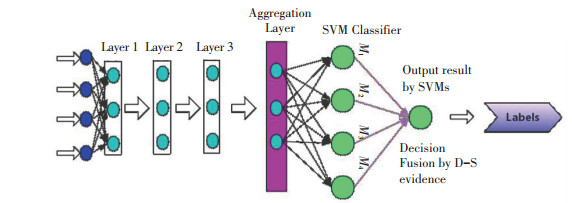 Fig.3 Structure with SVM classifiers
 2.4 Training Process of Improved SDA Assume that the input layer dimension is m, the number of hidden layers is l, and the network of each layer is marked as n1, n2, ..., nl. As the depth increased, the training duration also increased, which is described in Table 1.
表 1
Step 1Calculate the outputs of layers in the forward direction from the first hidden layer.
Step 2Use output(s) of the previous layer to train the next layer. Sequentially, train the output value, weight, and bias according to sample data until the (l-1)th layer.
Step 3Use the output of the (l-1)th layer nodes as the input of the lth layer.
Step 4Connect the trained network into two parts: encoder and decoder. The encoder part is the network from data input to the output of the final DA network, which is positive propagation. The decoder part is the network from the final auto encoding network to the original input data, which is reverse propagation.
Step 5Set different proportions and aggregate information for training and testing data.
Step 6Select the hidden node of the aggregation layer as the input of SVM. Train the SVM and adjust SVM parameters. So far, the whole ISDA process is completed.
Table 1 Back propagation learning procedure for the ISDA model
3 Fault Classification Applications Rolling bearings are important elements in rotary machinery components, and fault classification often plays an essential role in their performance and reliability[19]. Thus, the proposed fault diagnosis approach was used in rolling bearing with different noise and working conditions as an example. Fault classification using the proposed ISDA approach was compared with existing diagnosis algorithms, and the detailed results are listed below. Rolling bearing datasets employed in the experiments were obtained from the Bearing Data Center of CWRU[20]. The ISDA model was established based on a deep learning toolbox as indicated in Ref.[21]. All the experiments were conducted under the TensorFlow environment.
3.1 Experiment Description The datasets composed of multivariate vibration series were generated by a bearing test-rig as shown in Fig. 4. The experiment used an acceleration sensor to collect vibration signals. The sensor was mounted on the motor housing by using a magnetic base, and the data was obtained when the bearing was in normal, outer race fault, inner race fault, and rolling fault states under loads of 0 HP and 2 HP. The fault diameter of all fault states was 0.007″, and the speed of bearing revolution was 1 797 r/min and 1 750 r/min, respectively. The sampling point at the driving end and the sampling frequency was 12 kHz.
Fig.4
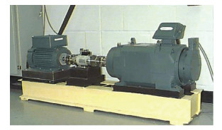 Fig.4 Bearing test rig used for experiment
 In the experiment, fault diameter of 0.007″ was used, and loads 0 HP and 2 HP were chosen from dataset. Detailed information is listed in Table 2.
表 2
(HP)Fault diameter
(mm)Speed of
revolution
(r/min)Samples
(unit)Tag
Normal0
2None
None1 797
1 750203
4040
1
Inner race0
20.007
0.0071 797
1 750101
1012
3
Outer race0
20.007
0.0071 797
1 750101
1014
5
Rolling0
20.007
0.0071 797
1 750102
1066
7
Table 2 Bearing information
3.2 Data Processing and Health State Definition The Drive End (DE) accelerometer data of the normal (ID: 97, 99), inner race fault (ID: 105, 107), rolling element fault (ID: 118, 120), and outer race fault (ID: 130, 132) conditions were acquired for classification.
Since vibration signals need to be inputted to the neural network and the activation function in the neural network needs to transform the features into the data of [0, 1] interval distribution, the following normalization is required:
${x_{io}} = \frac{{{x_i} - {x_{\min }}}}{{{x_{\max }} - {x_{\min }}}}$ (10)
where xio indicates the i-th feature parameter after the normalization, and xi is the i-th feature parameter after the preprocessing, while xmin and xmax are the minimum and maximum values of the current feature parameters, respectively. Finally, to improve the noise processing capability of the algorithm in practical application, random noises with mean value 0 were added to the data, in which 70% of each sample was taken as the training set, 15% as the verification set, and 15% as the test set.
3.3 Established Model An established optimal ISDA model had an impact on the diagnosis effect. Considering the stack characteristics of the deep learning process, the study in Ref.[21] conveys several parameters that have an important influence on the unsupervised learning process. In this section, receptive input size, numbers of hidden layers and units were tested to determine the optimal values in ISDA model. Reconstruction errors of auto-encoders were set to be the indicators for judging the employed parameters. Training set was used to provide data for reconstruction algorithm.
The reconstruction error
$L\left( {{\mathit{\boldsymbol{x}}^d},{{\mathit{\boldsymbol{\hat x}}}^d}} \right) = \frac{1}{2}{\left\| {{\mathit{\boldsymbol{x}}^d} - {{\mathit{\boldsymbol{\hat x}}}^d}} \right\|^2}$ (11)
$J\left( {\mathit{\boldsymbol{W}},\mathit{\boldsymbol{b}}} \right) = \left[ {\frac{1}{M}\sum\limits_{d = 1}^M L \left( {{\mathit{\boldsymbol{x}}^d},{{\mathit{\boldsymbol{\hat x}}}^d}} \right) + \frac{\lambda }{2}\sum\limits_{l = 1}^{{n_l} - 1} {\sum\limits_{i = 1}^{{s_l}} {\sum\limits_{j = 1}^{{s_{l + 1}}} {{{\left( {W_{ji}^l} \right)}^2}} } } } \right]$ (12)
3.3.1 Input size of receptive vector In general cases, the larger the input data is, the better the representations are. However, the receptive input size needs to be set based on computational constraints. To observe the changing influence, the experiment was first conducted based on the first auto-encoder, as shown in Fig. 5. The reconstruction error clearly deceased when larger receptive input size ranged from 100 to 600. However, the subsequent values were rather stable and less than 0.12, when the receptive input size was greater than 550, which means that employed input features covered enough information. Therefore, nodes of the aggregate layer were set to 550.
Fig.5
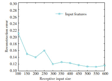 Fig.5 Receptive input size
 3.3.2 Number of hidden layers and nodes Hidden nodes are important to achieve high performance in the ISDA model, so does the depth of deep architecture. Take the example of two auto-encoders (i.e., SDA and improved algorithm) into account, where input size was set to 550 based on the experiment above, as illustrated in Fig. 6. It was noted that the two algorithms seemed to be satisfactory when the nodes were greater than 130. However, the SDA got the least reconstruction error which was 160, and ISDA was 150 (taking the last hidden layer into account). That is because with the aggregate layer, more information can be directly conveyed by the last layer without previous layers.
Fig.6
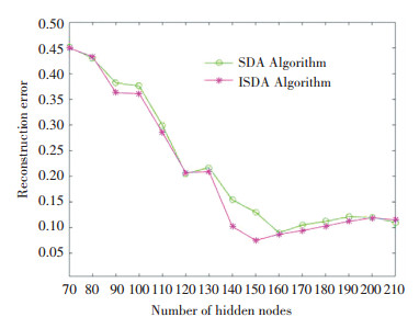 Fig.6 Number of hidden nodes of two algorithms
 By taking all the experimental results into account, further experiments of multiple hidden layers of two algorithms were conducted to demonstrate the effectiveness of ISDA. Conditions of each experiment are listed in Table 3.
表 3
input sizeHidden
layersHidden
nodesReconstruction
error
55021600.250 3
55031600.239 7
SDA55041600.177 5
algorithm55051600.155 1
55061600.074 9
55071600.073 8
55021500.211 9
55031500.178 6
55041500.148 8
ISDA
algorithm55051500.094 1
55061500.069 5
55071500.068 3
55081500.068 2
Table 3 Experi mental result comparison of two methods with different hidden layers
In Table 3, it can be found that changing with a different number of hidden layers is not clear and the expectation was that the number of hidden layers would be greater than 6. However, compared with SDA, by using the improved SDA algorithm, lower error levels were achieved in general with 7 or 8 hidden layers. Both algorithms reached lower errors of approximately 0.070 (7%), meaning that they are capable of mining salient bearing feature representations. Thus, 7 or 8 layers with 150 hidden units were employed. Since they have 8 different bearing operating states, the output layer has 8 nodes.
4 Bearing Diagnosis with Improved SDA As stated above, the method in this section is used to extract the hidden layer features of the test data. The outputs of the hidden layer of the trained model were extracted. In general, the fault characteristic of self-learning could be regarded as a type of dimension reduction process[22]. To verify the expressive ability of the extracted features, the principal component analysis (PCA)[23] method was used to extract the first three main components for visual analysis. Here, BP algorithm, RNN algorithm, and SDA algorithm were used to process the data set, where the fault diameter is 0.007″(mm). The visual analysis results were compared, as presented in Figs. 7-9 (Note: 7 layers are shown in Fig. 8(a) and Fig. 9(a), and 8 layers are shown in Fig. 8(b) and Fig. 9(b), in which dots of same color represent a category).
Fig.7
 Fig.7 PCA graph of PB
 Fig.8
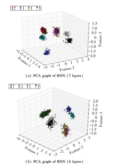 Fig.8 PCA graph of RNN
 Fig.9
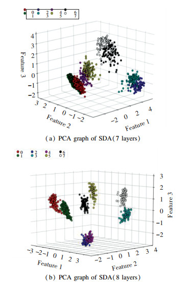 Fig.9 The PCA graph of SDA
 Fig. 7 illustrates the output of the single-llayer BP neural network hidden layer node, which was processed by PCA. Figs. 8(a) and (b) show the processing of the 7th and the 8th hidden layer nodes by SDA. Figs. 9(a) and (b) show the processing of the outputs of the 7th and the 8th hidden layer nodes by ISDA. The faults can be clearly differentiated in Fig. 7, but it is difficult to distinguish the different working conditions of each fault, indicating that the original information was not very well classified. In Figs. 8-9, faults were clearly classified even when the number of layers increased. However, the distinction between working conditions 0, 1, 4, 5 was still insufficient. Based on Fig. 9, Fig. 10 shows that the faults of working conditions 0, 1, 4, 5 were accurately classified and each feature was highlighted, suggesting the improvement of the classification accuracy. Another experiment utilized the data in Table 2, but added with different types of noise, with the learning rate of gradient descent set to 0.01, the times of pre-training to 25, and the fine tuning to 50 cycles, as shown in Table 4. The classification rate can be performed as follows:
${A_{{\text{cc}}}} = \frac{{{U_{{\text{predict}}}} - {U_{{\text{actual}}}}}}{{{U_{{\text{total}}}}}} \times 100\% $ (13)
Fig.10
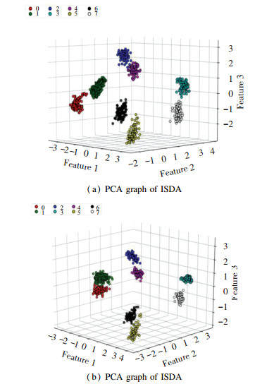 Fig.10 PCA graph of ISDA
 表 4
SNR is
14 dBSNR is
15 dBSNR is
16 dBSNR is
17 dBSNR is
18 dB
BP70.1271.1872.7574.2576.75
RNN87.6788.1592.2192.7393.65
SDA93.4393.5194.6595.1196.82
ISDA93.5893.7594.8395.7597.02
Table 4 Classification results
where Upredict are the classifications from test set, Uactual are the correct labels, and Utotal are the total numbers of test set.
From the diagnosis table, methods of RNN, SDA, and ISDA exhibited high correct classification rates of above 85%. However, SDA and ISDA produced relatively higher accuracy and stability in most cases for different SNRs owing to their ability of dealing with complex non-linear data. Moreover, compared with SDA, it seems that the data destruction process in ISDA was superior in terms of bearing diagnosis under the working conditions of strong space noise, with an accuracy improvement of 0.64% at 17 dB as an example. Also note that, the RNN algorithm had good anti-noise ability when SNR changed from 15 dB to 16dB, as shown in Fig. 11.
Fig.11
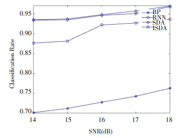 Fig.11 Methods with different SNRs
 Fig. 12 shows the training time for each algorithm, which became shorter when SNR increased from 14 dB to 18 dB. The training time was 371 s, 368 s, 376 s, and 64 s for ISDA, SDA, RNN, and BP at 18 dB. However, at 14 dB, the calculation time increased to 396 s, 398 s, 403 s, and 67 s, respectively. As mentioned above, the proposed method could achieve better diagnosis performance but it seems to be more time-consuming than other methods. It can be explained by their learning and back propagation mechanisms with aggregation layer. It is worth mentioning that compared with SDA at 14 dB, the improved algorithm received relatively less training time because the aggregate layer could contain previous information and data destruction could reduce back propagation time with better robustness.
Fig.12
 Fig.12 Training time for different methods
 5 Conclusions A classification algorithm using SVM with ISDA is proposed in this paper to reduce classification error and improve accuracy of rolling bearing. The classification accuracy may be influenced due to samples with noises. ISDA algorithm was used to extract features automatically, while BP and RNN algorithms need vibration signals, and a wide set of features were used as the inputs in the neural network models. Aggregate layers can make different features of layers together to get better expression of information. This method effectively divided different features of rolling bearing with different SNRs. The experimental results demonstrated the effectiveness of the proposed approach by comparing with the traditional BP, RNN, and SDA. The diagnostic result showed that ISDA had better generalized performance, higher diagnostic accuracy, and stronger robustness than other algorithms.
At the same time, the optimal parameter determination such as learning rate and the choosing of parameters of classifiers are still challenges for the further improvement of this paper.
References
[1] Lyu Feiya, Wen Chenglin, Bao Zejing, et al. Fault diagnosis based on deep learning. American Control Conference (ACC). Piscataway: IEEE, 2016.1-16. DOI: 10.1109/ACC.2016.7526751. (
 0)
0)[2] EI-Thalji I, Jantuman E. A summary of fault modeling and predictive health monitoring of rolling bearings. Mechanical Systems and Signal Processing, 2015, 60-61: 252-272. DOI:10.1016/j.ymssp.2015.02.008 (
 0)
0)[3] Li Min, Yang Jianhong, Wang Xiaojing. Fault feature extraction of rolling bearing based on an improved cyclical spectrum density method. Chinese Journal of Mechanical Engineering, 2015, 28(6): 1240-1247. DOI:10.3901/CJME.2015.0522.074 (
 0)
0)[4] Chen Jian. Fault Diagnosis for Rolling Bearing based on Fuzzy Rough Set and Artificial Neural Network. Chengdu: Southwest Jiaotong University, 2012 (
 0)
0)[5] Jegadeeshwaran R, Sugnmaran V. Fault diagnosis of automobile hydraulic brake system using statistical features and support vector machines. Mechanical Systems and Signal Processing, 2015, 52-53: 436-446. DOI:10.1016/j.ymssp.2014.08.007 (
 0)
0)[6] Zhang Xiaoli, Chen Wei, Wang Baojian, et al. Intelligent fault diagnosis of rotating machinery using support vector machine with ant colony algorithm for synchronous feature selection and parameter optimization. Neurocomputing, 2014, 167: 260-279. DOI:10.1016/j.neucom.2015.04.069 (
 0)
0)[7] Yang B S, Di Xiao, Han Tian. Random forest classifier for machine fault diagnosis. Journal of Mechanical Science and Technology, 2008, 22(9): 1716-1725. DOI:10.1007/s12206-008-0603-6 (
 0)
0)[8] Wang Z, Lu C, Ma J, et al. Novel method for performance degradation assessment and prediction of hydraulic servo system. Scientia Iranica B, 2015, 22(4): 1604-1615. (
 0)
0)[9] Bengio Y, Courville A, Vincent P. Representing learning: A review and new perspectives. Pattern Analysis and Machine Intelligence, 2013, 35(8): 1798-1821. DOI:10.1109/TPAMI.2013.50 (
 0)
0)[10] Wang X X, Wang Y. Improving content-based and hybrid music recommendation using deep learning. In Proceedings of the ACM International Conference on Multimedia. New York: ACM, 2014: 627-636. DOI: 10.1145/2647868.2654940. (
 0)
0)[11] Chen M, Weinberger K, Sha F, et al. Marginalized denoising auto-encoders for non-linear representations. Proceedings of the 31st International Conference on Machine Learning. Beijing, 2014.1476-1484 (
 0)
0)[12] Gehring J, Miao Yajie, Metze F, et al. Extracting deep bottleneck features using stacked auto-encoders. Proceedings of the 26th IEEE international Conference on Acoustics, Speech and Signal Processing. Piscataway: IEEE, 2013. 3377-3381 (
 0)
0)[13] Zhang Jinde, Cheng Junsheng, Yang Yu, et al. A rolling bearing fault diagnosis method based on multi-scale fuzzy entropy and variable predictive model baaed class discrimination. Mechanism and Machine Theory, 2014, 78: 187-200. DOI:10.1016/j.mechmachtheory.2014.03.014 (
 0)
0)[14] Bengio Y, Lee H. Editorial introduction to the neural networks special issue on deep learning of representation. Neural Networks, 2015, 64: 1-3. DOI:10.1016/j.neunet.2014.12.006 (
 0)
0)[15] LeCun Y, Bengio Y, Hinton G. Deep learning. Nature, 2015, 521: 436-443. DOI:10.1038/nature14539 (
 0)
0)[16] Vincent P, Larochelle H, Lajoie I, et al. Stacked denoising auto-encoders: Learning useful representations with D-S theory in a deep network with a local denoising criterion. Journal of Machine Learning Research, 2010, 11: 3371-3408. (
 0)
0)[17] Wang Yasi, Yao Hongxun, Zhao Sicheng. Auto-encoder based dimensional reduction. Neurocomputing, 2016, 184: 232-242. DOI:10.1016/j.neucom.2015.08.104 (
 0)
0)[18] Jiao Zaibin, Gong Heteng, Wang Yifei. A D-S evidence theory-based relay protection system hidden failure detection method in smart grid. IEEE Transactions on Smart Grid, 2006(99): 1-10. DOI:10.1109/TSG.2016.2607318 (
 0)
0)[19] Zhang Li, Zhao Jiaqiang, Zhang Xunan, et al. Study of a new improved PSO-BP neural network algorithm. Journal of Harbin Institute of Technology (New Series), 2013, 20(5): 106-112. DOI:10.11916/j.issn.1005-9113.2013.05.019 (
 0)
0)[20] Bearing Data Center of Case Western Reserve University. http://blog.csdn.net/x5675602/article/details/51315044.[2017-10-02] (
 0)
0)[21] Rasmusbergplam. Deep Learning Toolbox. https://github.com/rasmusbergpalm/DeepLearnToolbox#deeplearntoolbox.[2017-10-02] (
 0)
0)[22] Yang Yang, Shu Quang, Shanh M. Semi-supervised learning of feature hierarchies for object detection in a video. Proceedings of the IEEE Conference on Computer Vision and Pattern Recognition, 2013.1650-1657. DOI: 10.1109/CVPR.2013.216. (
 0)
0)[23] Weingessel A, Hornik K. Local PCA algorithms. IEEE Transactions on Neural Networks, 2000, 11(6): 1242-1250. DOI:10.1109/72.883408 (
 0)
0)