Yong Wang,Rongzheng Zhang
(Research Institute of Electronic Engineering Technology, Harbin Institute of Technology, Harbin 150001, China)
Abstract:
Through the coherent accumulation of target echoes, inverse synthetic aperture radar (ISAR) imaging achieves high azimuth resolution. However, because of the instability of the radar system, the echoes of the lSAR will be randomly lost. The conventional FFT processing methods can cause image blur and high sidelobes or other issues. A novel algorithm for ISAR missing-data imaging based on the Iterative Adaptive Approach (IAA) is proposed. The algorithm enjoys global convergence properties and does not need to set the parameters in advance. The missing-data ISAR imaging results for simulated and measured data illustrate the effectiveness of the algorithm.
Key words: iterative adaptive approach missing-data ISAR
DOI:10.11916/j.issn.1005-9113.17164
Clc Number:TN957.51
Fund:
Yong Wang, Rongzheng Zhang. ISAR Imaging of Missing Data Based on the Iterative Adaptive Approach[J]. Journal of Harbin Institute of Technology (New Series), 2018, 25(4): 41-47. DOI: 10.11916/j.issn.1005-9113.17164.

Fund Sponsored by the National Natural Science Foundation of China (Grant Nos. 61471149 and 61622107) Corresponding author Yong Wang, Winner of the National Science Fund for Excellent Youth Scholars and the Program for New Century Excellent Talents in University of Ministry of Education. E-mail: wangyong6012@hit.edu.cn Article history Received: 2017-12-20
Contents Abstract Full text Figures/Tables PDF
ISAR Imaging of Missing Data Based on the Iterative Adaptive Approach
Yong Wang

 , Rongzheng Zhang
 Research Institute of Electronic Engineering Technology, Harbin Institute of Technology, Harbin 150001, China
Received: 2017-12-20
Fund: Sponsored by the National Natural Science Foundation of China (Grant Nos. 61471149 and 61622107)
Corresponding author: Yong Wang, Winner of the National Science Fund for Excellent Youth Scholars and the Program for New Century Excellent Talents in University of Ministry of Education. E-mail: wangyong6012@hit.edu.cn
Abstract: Through the coherent accumulation of target echoes, inverse synthetic aperture radar (ISAR) imaging achieves high azimuth resolution. However, because of the instability of the radar system, the echoes of the lSAR will be randomly lost. The conventional FFT processing methods can cause image blur and high sidelobes or other issues. A novel algorithm for ISAR missing-data imaging based on the Iterative Adaptive Approach (IAA) is proposed. The algorithm enjoys global convergence properties and does not need to set the parameters in advance. The missing-data ISAR imaging results for simulated and measured data illustrate the effectiveness of the algorithm.
Key words: iterative adaptive approach missing-data ISAR
1 Introduction The ISAR imaging system transmits wideband signals to improve the range resolution, and improves the azimuth resolution by the coherent accumulation of the target echo. In practice, there is various perturbation factors that make the data received in the azimuth direction missing[1]. However, the instability of the radar system may cause radar echo randomly lost. At this point, the use of traditional FFT methods will lead to the target defocus and other issues, resulting in unidentifiable imaging results.
At present, the main method for ISAR imaging of missing data is the Compression Sensing (CS)[2-4], such as an iterative or non-iterative Orthogonal Matching Pursuit(OMP)[5] algorithm. As long as the signal satisfies a certain sparsity level, the time-domain can be sampled at a sampling frequency lower than the Nyquist theorem, so that the signal can be approximately reconstructed with high efficiency. However, the algorithm needs to predict the sparsity level of the signal, and when the percentage of missing is large, the recovery performance will be severely degraded.
Since the core issue is using the missing data to estimate the spectrum of the signal in each range unit, the spectral estimation algorithms can be used for ISAR imaging. In the past few years, modern spectral estimation algorithms have been widely used for ISAR super-resolution imaging[6-10]. As a branch of modern spectral estimation method, adaptive spectral estimation has been greatly developed recently. Among them are the Capon[11] and the Amplitude and Phase Estimation of a Sinusoid (APES)[12-13], which both perform spectrum estimation by adaptively constructing a filter bank.
Recently, the non-parametric weighted least-squares Iterative Adaptive Approach (IAA)[14-15] has further improved the accuracy of the adaptive spectral estimation method. IAA constructs the signal covariance matrix using the spectral estimation results of the previous iteration and takes its inverse matrix into the weighted least-squares optimization problem. Because this method is suitable for non-uniform sampling of data, IAA is applied to recover missing data[16]. The method is not affected by the signal parameters, the signal can be recovered in the case of a large proportion of missing data, accurate imaging with small rotational angle[10]. In this paper, we use IAA for missing data ISAR imaging. Using IAA for the azimuth compression of missing data can effectively solve the problem of spectrum leakage. The imaging results of simulated and measured data illustrate the effectiveness of IAA.
Structure of this paper: In Section 2, the ISAR imaging principle and the random missing data model is presented; Section 3 presents IAA; In Section 4, the ISAR missing-data imaging results based on IAA are presented, and through the comparison with OMP illustrates the superiority of IAA; Section 5 is the conclusion of the paper.
2 ISAR Imaging Principle and ISAR Random Missing Data Model In order to improve the range resolution, the radar usually emits wideband signals and the most widely used is the linear frequency modulated (LFM) signal. We set the pulse emitting time as tm=mT, m=0, 1, 2, ... is the slow time and the fast time is
$s\left( {\hat t,{t_m}} \right) = rec{t_{{T_p}}}\left( {\hat t} \right)\exp \left[ {{\rm{j}}2{\rm{ \mathsf{ π} }}\left( {{f_c}t + \frac{1}{2}k{{\hat t}^2}} \right)} \right]$ (1)
where k is the frequency modulation slope, fc is center frequency, rectTp(u) is a rectangular window of width Tp. Let the distance between the scattering points and the radar is Ri, the echo is:
$\begin{array}{*{20}{c}}{{s_r}\left( {\hat t,{t_m}} \right) = \sum\limits_{i = 1}^K {{A_i}} \cdot rec{t_{{T_p}}}\left( {\hat t} \right)\exp \left[ {{\rm{j}}2{\rm{ \mathsf{ π} }}\left( {\hat t - } \right.} \right.}\\{\left. {\left. {\frac{{2{R_i}\left( {{t_m}} \right)}}{c}} \right) + \frac{1}{2}k{{\left( {\hat t - \frac{{2{R_i}\left( {{t_m}} \right)}}{c}} \right)}^2}} \right]}\end{array}$ (2)
The signal after pulse compression by STRETCH processing in the fast time is:
$\begin{array}{*{20}{c}}{{S_r}\left( {\hat f,{t_m}} \right) = \sum\limits_{i = 1}^K {{A_i}} \cdot {\rm{sinc}}\left[ {{T_p}\left( {\hat f - \frac{{2k\mathit{\Delta }{R_i}\left( {{t_m}} \right)}}{c}} \right)} \right] \cdot }\\{\exp \left[ {\frac{{ - {\rm{j}}4{\rm{ \mathsf{ π} }}\mathit{\Delta }{R_i}\left( {{t_m}} \right)}}{\lambda }} \right]}\end{array}$ (3)
where λ is the wavelength of the transmitted signal, ΔRi(tm) is the distance between each scattering point and the reference point. After the motion compensation, the turntable imaging geometry is shown in Fig. 1.
Figure 1
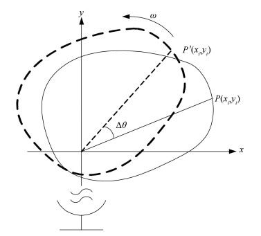 Figure 1 The turntable imaging geometry
 In Fig. 1, ω is the angular velocity of rotation, the relative distance can be expressed as
$\mathit{\Delta }{R_i}\left( {{t_m}} \right) = {x_i}\sin \left( {\omega {t_m}} \right) + {y_i}\cos \left( {\omega {t_m}} \right)$
If tm is very small, then we can obtain
$\sin \left( {\omega {t_m}} \right) \approx \omega {t_m},\cos \left( {\omega {t_m}} \right) \approx 1$
Therefore, at a slow time, the signal within each range cell can be represented as the sum of the single frequency signals:
$s\left( {{t_m}} \right) = \sum\limits_{i = 1}^K {{\sigma _i}\exp \left( {\frac{{ - {\rm{j}}4{\rm{ \mathsf{ π} }}{x_i}\omega {t_m}}}{\lambda }} \right)} $ (4)
If the signal s(tm) in each range cell is converted to the Doppler domain, the distribution of the scattering points in the azimuth can be obtained. In practice, there is various perturbation factors that make the data received in the azimuth direction appear missing. When part of the echo is missing, the signal at slow time can be expressed as[2]:
${s_g}\left( {{m_g}} \right) = \sum\limits_{i = 1}^K {{\sigma _i}\exp \left( {\frac{{ - {\rm{j}}4{\rm{ \mathsf{ π} }}{x_i}\omega {m_g}}}{\lambda }} \right)} $ (5)
where {mg}g=1G are the receipt times of valid data. At this point, if we still use the fast Fourier transform to analyze the Doppler spectrum of the signal, there will be serious spectrum leakage.
3 Weighted Least-Squares Iterative Adaptive Approach As aforementioned analysis, the missing data imaging problem can be translated into spectral estimation of non-uniformly sampled signal sg. Let K denote the number of sampling points in the frequency domain. Usually, K is more than the number of the points in the time domain. Let:
${\mathit{\boldsymbol{A}}_g} = \left[ {{\mathit{\boldsymbol{a}}_g}\left( {{\omega _1}} \right), \cdots ,{\mathit{\boldsymbol{a}}_g}\left( {{\omega _K}} \right)} \right]$ (6)
${\mathit{\boldsymbol{a}}_g}\left( {{\omega _k}} \right) = \left[ {\exp \left( {{\rm{j}}{\omega _k}{m_1}} \right), \cdots ,\exp \left( {{\rm{j}}{\omega _k}{m_G}} \right)} \right]$ (7)
where {ag(ωk)}k=1K is the Fourier vectors corresponding to sg at {ωk}k=1K. The valid data sg can be modeled as:
${\mathit{\boldsymbol{s}}_g} = {\mathit{\boldsymbol{A}}_g}\mathit{\boldsymbol{\alpha }} + e$ (8)
where α= [α(ω1), ..., α(ωK)]T is the vector of complex spectral amplitudes at frequency {ωk}, e is Gaussian complex noise, (·)T denotes the transpose. Assuming that the signal is not correlated with noise, the noise and interference covariance matrix for the valid data can be defined as:
$\mathit{\boldsymbol{Q}} = {\mathit{\boldsymbol{R}}_g} - {\left| {\alpha \left( {{\omega _k}} \right)} \right|^2}{\mathit{\boldsymbol{a}}_g}\left( {{\omega _k}} \right)\mathit{\boldsymbol{a}}_g^ * \left( {{\omega _k}} \right)$ (9)
$\mathit{\boldsymbol{R}} = \sum\limits_{k = 1}^K {{{\left| {\alpha \left( {{\omega _k}} \right)} \right|}^2}{\mathit{\boldsymbol{a}}_g}\left( {{\omega _k}} \right)\mathit{\boldsymbol{a}}_g^ * \left( {{\omega _k}} \right)} = \mathit{\boldsymbol{AP}}{\mathit{\boldsymbol{A}}^ * }$ (10)
where (·)* denotes conjugate transpose, R is the covariance matrix of the valid data, P is a K × K diagonal matrix of diagonal elements {|α(ωk)|2}k=1K of signal power at frequency {ωk}. The weighted least square (WLS) estimation is used to estimate the complex amplitudes {α(ωk)}k=1K, and the following optimization problem is obtained:
$\mathop {\min }\limits_{\alpha \left( {{\omega _k}} \right)} {\left( {{\mathit{\boldsymbol{s}}_g} - \alpha \left( {{\omega _k}} \right){\mathit{\boldsymbol{a}}_g}\left( {{\omega _k}} \right)} \right)^ * }{\mathit{\boldsymbol{Q}}^{ - 1}}\left( {{\mathit{\boldsymbol{s}}_g} - \alpha \left( {{\omega _k}} \right){\mathit{\boldsymbol{a}}_g}\left( {{\omega _k}} \right)} \right)$ (11)
$\hat \alpha \left( {{\omega _k}} \right) = \frac{{{\mathit{\boldsymbol{a}}^ * }\left( {{\omega _k}} \right){\mathit{\boldsymbol{Q}}^{ - 1}}{\mathit{\boldsymbol{s}}_g}}}{{{\mathit{\boldsymbol{a}}^ * }\left( {{\omega _k}} \right){\mathit{\boldsymbol{Q}}^{ - 1}}\mathit{\boldsymbol{a}}\left( {{\omega _k}} \right)}}$ (12)
The detailed implementation of it can be found in Ref. [16]. Using matrix inversion lemma, we can simplify Eq. (12) to:
$\hat \alpha \left( {{\omega _k}} \right) = \frac{{{\mathit{\boldsymbol{a}}^ * }\left( {{\omega _k}} \right){\mathit{\boldsymbol{R}}^{ - 1}}{\mathit{\boldsymbol{s}}_g}}}{{{\mathit{\boldsymbol{a}}^ * }\left( {{\omega _k}} \right){\mathit{\boldsymbol{R}}^{ - 1}}\mathit{\boldsymbol{a}}\left( {{\omega _k}} \right)}}$ (13)
Using the iterative method, first let P be the unit matrix as the initial value, and then calculate R by Eq.(10) and
Step 1??Find the receipt times {mg}g=1G of valid data Sg, construct the Fourier matrix A in the form of Eq.(6).
Step 2??Set P as the unit matrix, calculate the initial value of the covariance matrix R by Eq.(10).
Step 3??Calculate
Step 4??Calculate R by Eq. (10), return to the Step 3, until the iteration converges.
The computational cost of computing a one-dimensional signal using the proposed algorithm is N(2KG2+KG+G3)[17]. Where N is the number of iterations, G is the valid data length. The running time of the IAA algorithm is dominated by calculating the inverse of the covariance matrix. When valid data is large in length, iterations take a long time.
We simulate a multi-component complex sinusoidal signal, and use it to verify the missing data iterative adaptive method. The amplitude and frequency of these four complex sinusoidal signals are (0.5 Hz, 0.25 Hz), (1.0 Hz, 0.39 Hz), (1.5 Hz, 0.67 Hz), (1.5 Hz, 0.77 Hz). The number of sampling points is 100, and the complex Gaussian white noise with the mean value of 0 and variance 0.01 is added to the signal. To verify the ability of the IAA method to estimate line spectra with missing data, 50% of the data is randomly lost. Fig. 2(a) is the result of missing data spectrum estimated by FFT, it can be seen that the directly use of FFT will produce serious spectrum leakage. Fig. 2(b) is the result of IAA, it can be seen that the IAA algorithm can accurately estimate the spectrum of signal in the case of a large proportion of missing.
Figure 2
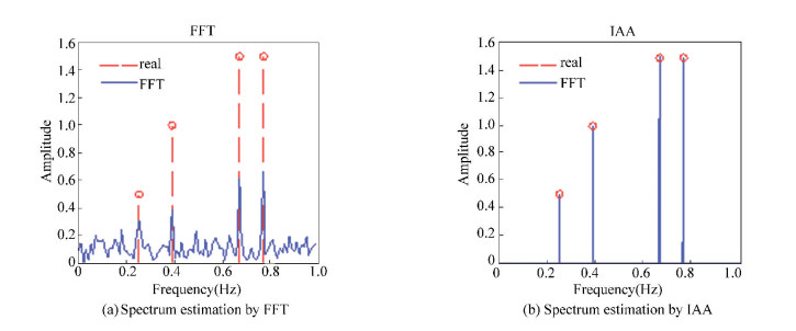 Figure 2 Result of missing data spectrum estimation by FFT and IAA
 4 ISAR Missing-Data Imaging Based on Iterative Adaptive Approach 4.1 Simulated Data Imaging To illustrate the superiority of the IAA algorithm in ISAR imaging, we used simulated MIG-25 data provided by the Naval Research Laboratory-ABD (NRL) for the missing data imaging experiments. The step frequency radar works at 9 GHz with a bandwidth of 512 MHz and the Pulse repetition frequency is 15 kHz. A total of 512 pulses, 64 samples are collected from each pulse. This experiment only takes the first 64 echoes, and randomly lost part of the echo. The proportions of missing data are 25%, 50% and 75%. Fig. 3 (a), (d) and (g) is the results of missing data imaging by FFT with 75%, 50% and 25% valid data, as expected, the distortion of the image becomes more and more serious as the valid data decreases, so we cannot obtain the information of the target; Fig. 3(b), (e) and (h) show the results of missing data imaging by IAA with 75%, 50% and 25% valid data, it can be seen that the IAA method can be used to get a clear image even in the absence of a large amount of echo, the image is enough to discern the shape of the target. Fig. 3(c), (f) and (i) are the results of missing data imaging by OMP with 75%, 50% and 25% valid data, it shows that OMP can also use missing data imaging, but the reduction effect is slightly worse than IAA.
Figure 3
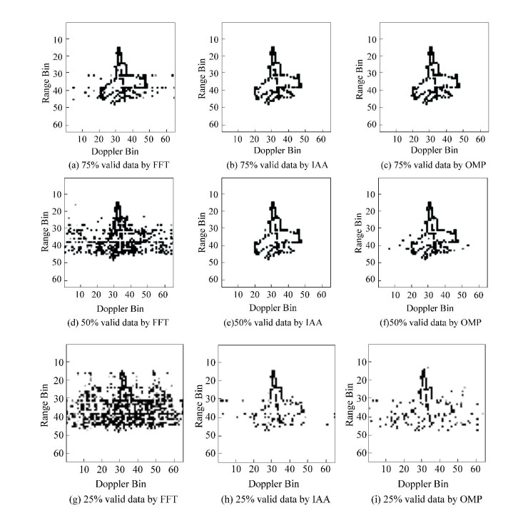 Figure 3 Result of simulated data imaging by FFT, IAA and OMP
 4.2 Measured Data Imaging To prove the validity of IAA method in practice, we used the real data from the Yak-42 plane to perform the missing data imaging experiment. The radar transmits a LFM signal at a carrier frequency of 5520 MHz with a bandwidth of 400 MHz. The pulse repetition frequency is 400 Hz and the pulse width is 25.6 μs. As with the previous data, we randomly discard some of the echoes. The proportions of missing data are 25%, 50% and 75%. Fig. 4(a), (d) and (g) are the results of missing data imaging by FFT with 75%, 50% and 25% valid data; Fig. 4(b), (e) and (h) show the results of missing data imaging by IAA with 75%, 50% and 25% valid data; Fig. 4(c), (f) and (i) is the results of missing data imaging by OMP with 75%, 50% and 25% valid data. It can be seen that both IAA and OMP can perform missing data imaging. Due to the sparseness of OMP algorithm, the resolution of the results is higher than that of IAA. However, the IAA has a clearer graphical outline, so the recovery capability is better.
Figure 4
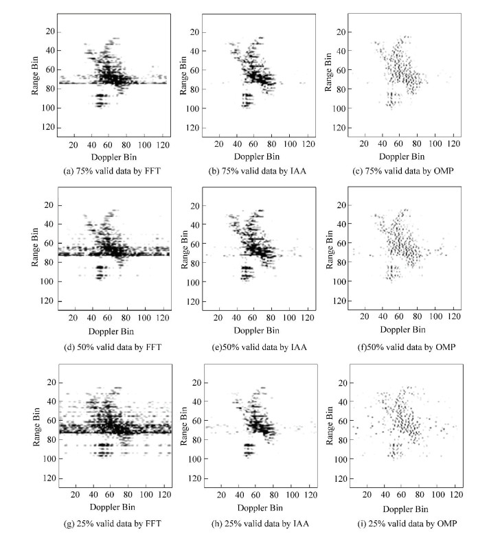 Figure 4 Result of real data imaging by FFT, IAA and OMP
 4.3 Imaging Effect Analysis The results of three methods of missing data imaging were quantitatively analyzed by correlation coefficients. The correlation coefficient of 2d image is defined as:
$r = \frac{{\sum\limits_{i = 1}^N {\sum\limits_{j = 1}^M {\left( {{a_{i,j}} - \bar a} \right)\left( {{b_{i,j}} - \bar b} \right)} } }}{{\sqrt {\sum\limits_{i = 1}^N {\sum\limits_{j = 1}^M {{{\left( {{a_{i,j}} - \bar a} \right)}^2}} } } \cdot \sqrt {\sum\limits_{i = 1}^N {\sum\limits_{j = 1}^M {{{\left( {{b_{i,j}} - \bar b} \right)}^2}} } } }}$ (14)
where
$\bar a = \frac{1}{{NM}}\sum\limits_{i = 1}^N {\sum\limits_{j = 1}^M {{a_{i,j}}} } ,\bar b = \frac{1}{{NM}}\sum\limits_{i = 1}^N {\sum\limits_{j = 1}^M {{b_{i,j}}} } $
where ai, j and bi, j are the grayscale of each point in the corresponding image. The correlation coefficient indicates the degree of correlation between two images. The larger the correlation coefficient is, the closer the two images are. Conversely, the smaller the correlation coefficient is, the greater the difference between the two images is. Therefore, in the case of using the same algorithm, the correlation coefficient between the missing data image and the corresponding complete data image indicates the ability of the algorithm for the missing data imaging. Here we use the simulated MIG-25 data in Section 4.1 to increase the data loss rate from 0 to 75%. For each data loss rate, the sampling loss time is randomly generated. 100 Monte Carlo experiments were performed to calculate the average correlation coefficient. The experimental results is shown in Fig. 5.
Figure 5
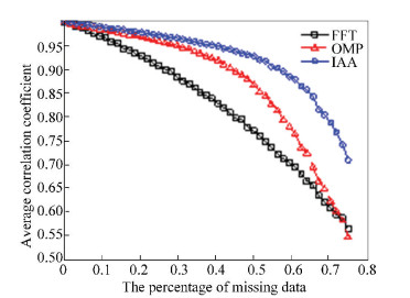 Figure 5 Average correlation coefficient of FFT, IAA and OMP
 The three curves in Fig. 5 show that the correlation coefficients between the original image and the restored image change with the missing data percentage when using FFT, IAA and OMP. When there is no missing data, the correlation coefficients of all three algorithms are 1, indicating that the two images are exactly the same. As the percentage of missing data increases, the correlation coefficient of the three algorithms starts to decline, indicating that images show different degrees of distortion. Overall, both IAA and OMP are better than FFT. When missing data is less than 40%, IAA's recovery is slightly better with OMP. When missing data is more than 40%, OMP's resilience declines rapidly because of the increased signal uncertainty over the transform domain as the missing data increases, and the signal will not satisfy the sparsity level. However, IAA's performance is relatively stable. Similar results are obtained for the measured data in Section 4.2.
5 Conclusions ISAR data loss may occur due to unstable radar systems and azimuth interference. The use of traditional FFT processing methods can lead to azimuth spectrum leakage. In this paper, an ISAR missing data imaging method based on IAA is proposed. The algorithm applies the weighted least squares estimation to obtain the spectrum of the non-uniformly sampled signal. The results of the simulated MIG-25 and the Yak-42 show that the algorithm can obtain a clear target image under the condition of random missing data.
References
[1] Larsson E G, Stoica P, Li Jian. Amplitude spectrum estimation for two-dimensional gapped data. In IEEE Transactions on Signal Processing, 2002, 50(6): 1343-1354. DOI:10.1109/TSP.2002.1003059 (
 0)
0)[2] Wang Y, Kang J, Zhang R. ISAR imaging with random missing observations based on non-iterative signal reconstruction algorithm. 2014 12th International Conference on Signal Processing (ICSP). Piscataway: IEEE, 2014, 1876-1879. DOI:10.1109/ICOSP.2014.7015318 (
 0)
0)[3] Ren Xiaozhen, Qiao Lihong, Qin Yao, et al. Sparse regularization based imaging method for inverse synthetic aperture radar. 2016 Progress in Electromagnetic Research Symposium (PIERS). Piscataway: IEEE, 2016, 4348-4351. DOI:10.1109/PIERS.2016.7735622 (
 0)
0)[4] Brajovi? M, Orovi? I, Dakovi? M, et al. The reconstruction of 2D sparse signals by exploiting transform coefficients variances. IEEE EUROCON 2017-17th International Conference on Smart Technologies. Piscataway: IEEE, 2017, 282-286. DOI:10.1109/EUROCON.2017.8011120 (
 0)
0)[5] Tropp J A, Gilbert A C. Signal recovery from random measurements via orthogonal matching pursuit. In IEEE Transactions on Information Theory, 2007, 53(12): 4655-4666. DOI:10.1109/TIT.2007.909108 (
 0)
0)[6] Freedman A, Steinberg B D, Chkhenkeli G. Applying the minimum free energy spectral estimation algorithm to ISAR imaging. 1996 IEEE International Conference on Acoustics, Speech, and Signal Processing, 1996.ICASSP-96. Conference Proceedings. Piscataway: IEEE, 1996, 2773-2776. DOI:10.1109/ICASSP.1996.550128 (
 0)
0)[7] Mayhan J T, Burrows M L, Cuomo K M, et al. High resolution 3D "snapshot" ISAR imaging and feature extraction. In IEEE Transactions on Aerospace and Electronic Systems, 2001, 37(2): 630-642. DOI:10.1109/7.937474 (
 0)
0)[8] Bon N, Khenchaf A, Garello R. Airborne scan mode ISAR imagery of ships using high resolution spectral methods and particle filter. IGARSS 2004. 2004 IEEE International Geoscience and Remote Sensing Symposium. Piscataway: IEEE, 2004, 2: 1506-1509. DOI:10.1109/IGARSS.2004.1368707 (
 0)
0)[9] Kalognomos G, Frangos P. Combining capon and APES noise covariance estimates for spectral estimation for ISAR applications. Proceedings of 2nd International Conference on Recent Advances in Space Technologies. Piscataway: IEEE, 2005, 694-698. DOI:10.1109/RAST.2005.1512656 (
 0)
0)[10] Hu P J, Xu S Y, Wu W Z, et al. IAA-based high-resolution ISAR imaging with small rotational angle. In IEEE Geoscience and Remote Sensing Letters, 2017, 14(11): 1978-1982. DOI:10.1109/LGRS.2017.2744989 (
 0)
0)[11] Capon J. High-resolution frequency-wavenumber spectrum analysis. In Proceedings of the IEEE, 1969, 57(8): 1408-1418. DOI:10.1109/PROC.1969.7278 (
 0)
0)[12] Stoica P, Li Hongbin, Li Jian. A new derivation of the APES filter. In IEEE Signal Processing Letters, 1999, 6(8): 205-206. DOI:10.1109/97.774866 (
 0)
0)[13] Palsetia M R, Li Jian. Using APES for interferometric SAR imaging. In IEEE Transactions on Image Processing, 1998, 7(9): 1340-1353. DOI:10.1109/83.709665 (
 0)
0)[14] He H, Li J, Stoica P. Spectral analysis of non-uniformly sampled data: A new approach versus the Periodogram. 2009 IEEE 13th Digital Signal Processing Workshop and 5th IEEE Signal Processing Education Workshop. Piscataway: IEEE, 2009, 375-380. DOI:10.1109/DSP.2009.4785952 (
 0)
0)[15] Yardibi T, Li J, Stoica P, et al. Source localization and sensing: A nonparametric iterative adaptive approach based on weighted least squares. In IEEE Transactions on Aerospace and Electronic Systems, 2010, 46(1): 425-443. DOI:10.1109/TAES.2010.5417172 (
 0)
0)[16] Stoica P, Li J, Ling J. Missing data recovery via a nonparametric iterative adaptive approach. IEEE International Conference on Acoustics, Speech and Signal Processing, 2009. ICASSP 2009. 2009.3369-3372.DOI: 10.1109/ICASSP.2009.4960347. (
 0)
0)[17] Glentis G O, Jakobsson A. Efficient implementation of iterative adaptive approach spectral estimation techniques. IEEE Transactions on Signal Processing, 2011, 59(9): 4154-4167. DOI:10.1109/TSP.2011.2145376 (
 0)
0)