Keyi Li, Xi Chen,Gongjian Zhou
(School of Electronics and Information Engineering, Harbin Institute of Technology, Harbin 150001, China)
Abstract:
Constrained modeling and state estimation have attracted much attention in recent years. This paper focuses on target motion modeling and tracking in road coordinates. An improved initialization method, which uses the optimal fusion of the position measurements in different directions, is presented for the constraint coordinate Kalman filter (CCKF). The CCKF is evaluated with a comprehensive comparison to the state-of-art linear equality constraint estimation methods. Numerical simulation results demonstrate the better performance of the CCKF. Then the interacting multiple model CCKF (IMM-CCKF) is proposed to manifest the advantages of the CCKF in complex motion modeling and state estimations. The effectiveness of the IMM-CCKF in maneuvering target tracking with spatial equality constraints is demonstrated by numerical experiments.
Key words: Ground Targets Motion modeling Road Constraints Initialization IMM
DOI:10.11916/j.issn.1005-9113.15261
Clc Number:TN953
Fund:
Keyi Li,Xi Chen,Gongjian Zhou. Complex Motion Modeling and State Estimation in Road Coordinates[J]. Journal of Harbin Institute of Technology, 2017, 24(1): 19-25. DOI: 10.11916/j.issn.1005-9113.15261.

Fund Sponsored by the National Natural Science Foundation of China (Grant No. 61201311) Corresponding author Gongjian Zhou, E-mail: zhougj@hit.edu.cn Article history Received: 2015-09-12
Contents Abstract Full text Figures/Tables PDF
Complex Motion Modeling and State Estimation in Road Coordinates
Keyi Li, Xi Chen, Gongjian Zhou


School of Electronics and Information Engineering, Harbin Institute of Technology, Harbin 150001, China
Received: 2015-09-12
Fund: Sponsored by the National Natural Science Foundation of China (Grant No. 61201311)
Corresponding author: Gongjian Zhou, E-mail: zhougj@hit.edu.cn
Abstract: Constrained modeling and state estimation have attracted much attention in recent years. This paper focuses on target motion modeling and tracking in road coordinates. An improved initialization method, which uses the optimal fusion of the position measurements in different directions, is presented for the constraint coordinate Kalman filter (CCKF). The CCKF is evaluated with a comprehensive comparison to the state-of-art linear equality constraint estimation methods. Numerical simulation results demonstrate the better performance of the CCKF. Then the interacting multiple model CCKF (IMM-CCKF) is proposed to manifest the advantages of the CCKF in complex motion modeling and state estimations. The effectiveness of the IMM-CCKF in maneuvering target tracking with spatial equality constraints is demonstrated by numerical experiments.
Key words: Ground Targets Motion modeling Road Constraints Initialization IMM
1 IntroductionRecently, dynamic system modeling and state estimation with equality constraints have attracted considerable attention, since the incorporation of state constraints will result in the improved performance and there indeed exists a host of real systems with various state constraints. The constraints can be abstracted from physical laws or mathematical properties[1]. For example, road constraints are common to vehicles travelling along the roads, in which their positions are constrained. Ground target tracking with road constraints is a typical equality constraints problem, when the road width can be ignored.
Great efforts have been made and as a result several effective methods of equality constrained estimation have been proposed[2-3]. There are four representative methods: model reduction[4-6], pseudo measurement[7-8], estimate projection[9-10] and the projection system[11-12].
The model reduction method transforms the original constrained state estimation problem to an unconstrained one by using the constraints on purpose to reduce the dimension of the system model[4-6]. Though it may have outstanding numerical stability and simplified computational complexity, the fact that physical meaning of the state variables might be lost[3, 13-14] cannot be ignored.
The pseudo measurement method simply treats the equality constraint as a new measurement without measurement noise which is perfect[7-8]. But the new measurement noise covariance is singular so there may be some numerical problems[3, 15].
The estimate projection method is projecting the unconstrained estimation onto the constraint surface[9-10]. This is of practical importance since the projective point is closer to the unconstrained estimate than any other points on the constraint surface. However, it does not mean that the projected point is close to the true constrained state. Consequently, this method cannot provide true optimal estimation[3].
The projection system method mainly has two kinds of implementation ideas. In Refs.[11] and [12], a conversion method is used to design the dynamic system which satisfies the constraints and the Kalman filter is employed for constrained state estimation. Direct elimination method is used to get constrained dynamic equations expected from unconstrained ones in Refs.[13], [15] and [16]. The projection methods mentioned above provide a new approach for constrained design and state estimation and really result in performance improvement. However the essential of all these means is using the existing unconstrained dynamic models to explore the issue of constrained system model and estimation[3]. In practical ground target tracking applications, target trajectory and motion are arbitrary and intensely complex, it may be arduous to get a satisfactory expression by conventional geographic coordinates space model, even if the interacting multiple model (IMM) method is adopted.
Besides the above four kinds of efforts, there is another work, the one-dimension (1D) motion model proposed by Yang et al.[17]. Target kinematic representation by using the arc-length of the road as a basic component is closer to the physical reality and is a promising method for tracking with spatial constraints. However, to our knowledge, there are few works following this idea. In Ref.[17], only simple motions on roads are considered and there is no in-depth study on the corresponding problems, such as filter initialization and so on. In Ref.[18], a more comprehensive solution to road target tracking based on the 1D motion model is presented, but only the motion with constant speed is explored. Accurate system modeling and state estimation for complex motion with constraints is still an open problem.
In this paper, the motion modeling of maneuvering targets on the road is explored and a comprehensive filtering method is presented. The complex motion modeling is carried out in the road coordinates and results in the one-dimensional state. The corresponding filtering method performs in the road coordinates and is referred to as constraint coordinates Kalman filter (CCKF) for generality. A new initialization method, which optimally fuses the redundant two-dimensional measurements to initial the one-dimensional state, is derived based on the scheme of minimum mean squared error for the CCKF. Then a comprehensive comparison of the performance of CCKF against those of the existing typical constraint estimation algorithms is presented. The advantage of one-dimension modeling is not only reflected in being close to physical reality, more to the point, it also makes the target trajectory and dynamic models mutually independent which greatly reduces the difficulty of studying complex motion problems in constrained space. The problem of tracking a target moving along a circular road with variable speed is taken as an example to discuss complex motion modeling and state estimation in road constraints. The interacting multiple model filter in constraint coordinate Kalman filter (IMM-CCKF) is proposed to estimate the maneuvering target states with road constraints. Numerical experiments demonstrate the effectiveness of the proposed initialization and filtering methods.
The rest of this paper is organized as follows. In Section 2, the CCKF, the two-dimension joint initialization and the IMM-CCKF are presented. Simulations are performed in Section 3 and the important conclusions are drawn in Section 4.
2 Constraint Coordinate Kalman Filter2.1 Modeling and State EstimationDifferent from the conventional motion modeling methods which express target kinematic models in the free ground coordinates, such as 2D or 3D Cartesian coordinates, the main idea of the constraint coordinate Kalman filter is considering the arc-length of the target on a road or constraint curve as a general coordinate. Target's motion can be expressed by the time evolution of the relative position and speed on the road or curve. This not only makes the motion modeling closer to the physical reality, but also makes the modeling of complex motions on road easier. In fact, the dynamic models of targets are now independent to the trajectory.
In this paper, the varying speed (VS) model is incorporated in addition to the constant speed (CS) model, which was the only motion model considered in the previous works[17-18], to express complex motions on the constraint curves.
Generally, it is difficult to provide an analytic expression of the arc-length of a road with complex shape. The solution of trajectory modeling here is similar to that in Ref.[17]. The straight and circular segments are used jointly to approximate the arcs of different curvatures[17].
The parameterizations of the straight and circular segments, as shown in Fig. 1, are described below.
Figure 1
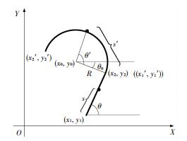 Figure 1 Parameterizations in road segments
 For linear segments, indispensable parameterizations are two pairs of points: the starting pair (x1, y1) and the ending pair (x2, y2). The length of the segment as well as its orientation can be calculated as
$\theta = {\tan ^{ - 1}}\left( {\frac{{{y_2} - {y_1}}}{{{x_2} - {x_1}}}} \right)$ (1)
$S = \sqrt {{{\left( {{x_2} - {x_1}} \right)}^2} + {{\left( {{y_2} - {y_1}} \right)}^2}} $ (2)
$S = \frac{{{x_2} - {x_1}}}{{\cos \theta }}$ (3)
$S = \frac{{{y_2} - {y_1}}}{{\sin \theta }}$ (4)
The states to be estimated are the arc-length or mileage count based vector, including its speed and acceleration. Denote the mileage count by s. Then we can obtain arbitrary points in this segment by
$\left\{ \begin{array}{l}x\left( s \right) = {x_1} + s\cos \theta \\y\left( s \right) = {y_1} + s\sin \theta \end{array} \right.$ (5)
where 0≤s≤S.
For curved segments, besides the starting pair (x1′, y1′) and the ending pair (x2′, y2′), we need circle center (x0, y0) to determine the initial angle and the radius of the circle as
${\theta _0} = {\tan ^{ - 1}}\frac{{{y_1}^\prime - {y_0}}}{{{x_1}^\prime - {x_0}}}$ (6)
$\begin{array}{l}R = \sqrt {{{\left( {{x_0} - {x_1}^\prime } \right)}^2} + {{\left( {{y_0} - {y_1}^\prime } \right)}^2}} = \\\;\;\;\;\;\;\sqrt {{{\left( {{x_0} - {x_2}^\prime } \right)}^2} + {{\left( {{y_0} - {y_2}^\prime } \right)}^2}} \end{array}$ (7)
$\mathit{\boldsymbol{ \boldsymbol{\varTheta} = }}{\cos ^{ - 1}}\left[ {1 - \frac{{{{\left( {{x_2}^\prime - {x_1}^\prime } \right)}^2} + {{\left( {{y_2}^\prime - {y_1}^\prime } \right)}^2}}}{{2{R^2}}}} \right]$ (8)
Similarly using s as the parameter, any point along the curved segment can be obtained by
$x\left( s \right) = {x_0} + R\cos \left( {{\theta _0} + \theta '} \right) = {x_0} + R\cos \left( {{\theta _0} + \frac{s}{R}} \right)$ (9)
$y\left( s \right) = {y_0} + R\sin \left( {{\theta _0} + \theta '} \right) = {y_0} + R\sin \left( {{\theta _0} + \frac{s}{R}} \right)$ (10)
where 0≤θ′≤Θ, θ0, R and Θ are given by Eqs.(6), (7) and (8), respectively.
Accordingly, it is expected that as long as a road of arbitrary shape can be approximated by linear and curved segments, we can invariably get any points along the road by
$\left\{ \begin{array}{l}x\left( s \right) = {g_x}\left( s \right)\\y\left( s \right) = {g_y}\left( s \right)\end{array} \right.$ (11)
where gx and gy are continuous functions of s, and 0≤s≤S.
Then we take several popular equality constrained estimation methods as comparisons. They are model reduction KF (MRKF)[4-6], pseudo measurement KF (PMKF)[7-8], estimate projection KF (EPKF)[9-10] and linear equality constraint KF (LECKF)[11-12].
The LECKF method constructed a LEC dynamic model which optimally fuses the linear equality constraint (LEC) and the unconstraint auxiliary dynamics. However, it may come over quite a few problems when the constraints are nonlinear, such as the multiple solutions problem and numerical problem. Moreover, the MMSE or LMMSE estimation of the constrained state may not obey the constraint in that condition[12].
Compared with these methods, CCKF has some outstanding advantages. Firstly, this method simplifies the kinematics model and it relates a tracking filter more closely to the physical reality. It also guarantees the target stay on the road and has only one degree of freedom (1DOF) along the road. That may be a hard task for the conventional motion modeling methods. Furthermore, it provides an effective way to introduce explicit constraints to state estimation. In other words, as long as the constraints can be explicitly represented, this method works. Finally we can see, in this method, the target trajectory is not determined by its velocity which means the dynamic models and target trajectory are mutually independent. This facilitates modeling of more complicated motion on the roads.
2.2 MeasurementsThe measurements are usually reported in sensor coordinates in real applications. For simplicity and focusing on the constraint problem, we assume that the measurements along the directions in ground coordinates are available[19-20]. The resulted methods in this paper can be extended to the sensor measurement case by taking the nonlinear transformation between Cartesian coordinates and sensor coordinates into account.
2.3 InitializationIn the problem of state estimation with equality constraints, the states in the whole duration are all expected to satisfy the constraints. However, most of the existing literatures concentrate the filtering procedure, while the initialization is not explored. In Refs. [8], [9] and [17], the true state value is used to initialize the filter, which is not practical in real applications. In the MRKF[4-6], PMKF[7-8] EPKF[9-10] and LECKF[11-12], the initialization problem is not discussed particularly. The conventional two-point difference initialization method can be used to start a filter in these methods based on Cartesian motion modeling[21]. However, the initialized states are not guaranteed to satisfy the constraints.
In this paper, a novel filtering initialization method is presented for the CCKF, using the minimum mean squared error fusion of the two dimensional measurements to improve the initial state accuracy and the filtering performance consequently. Additionally, the initialized states are constrained on the road.
In order to get the fusion results, we use the relationship between the mileage count and measurements in X or Y direction to calculate the one-dimension initialization ?x and ?y independently. Taking linear segment for example:
${{\hat s}_x} = g\left( x \right) = \frac{{x - {x_0}}}{{\cos \theta }}$ (12)
${{\hat s}_y} = g\left( y \right) = \frac{{y - {y_0}}}{{\sin \theta }}$ (13)
where x and y are the first two measurements, respectively. The variance of s in X and Y direction can be calculated by:
${\left( {\sigma _s^x} \right)^2} = {\left( {\frac{{\partial g}}{{\partial x}}} \right)^2}\sigma _x^2 = \frac{{\sigma _x^2}}{{{{\cos }^2}\theta }}$ (14)
${\left( {\sigma _s^y} \right)^2} = {\left( {\frac{{\partial g}}{{\partial y}}} \right)^2}\sigma _y^2 = \frac{{\sigma _y^2}}{{{{\sin }^2}\theta }}$ (15)
According to the minimum mean square error fusion method in Ref.[22], the fused state can be given by:
$\hat s = \frac{{{{\left( {\sigma _s^y} \right)}^2}}}{{{{\left( {\sigma _s^x} \right)}^2} + {{\left( {\sigma _s^y} \right)}^2}}}{{\hat s}_x} + \frac{{{{\left( {\sigma _s^x} \right)}^2}}}{{{{\left( {\sigma _s^x} \right)}^2} + {{\left( {\sigma _s^y} \right)}^2}}}{{\hat s}_y}$ (16)
Assuming σx=σy, then the joint initialization of ? in a linear segment can be written as
$\hat s = \cos \theta \cdot \left( {x - {x_0}} \right) + \sin \theta \cdot \left( {y - {y_0}} \right)$ (17)
And the corresponding variance is
$\sigma _s^2 = \frac{{{{\left( {\sigma _s^x} \right)}^2}{{\left( {\sigma _s^y} \right)}^2}}}{{{{\left( {\sigma _s^x} \right)}^2} + {{\left( {\sigma _s^y} \right)}^2}}}$
This initialization method is more reasonable than one-dimension measurements initialization in Eqs.(12) and (13). The redundant measurement in two-dimension are now fully utilized and information loss is avoided.
2.4 IMM-CCKFIn Refs.[20] and [23], CCKF is adopted under the assumption of constant target speed. But in realistic situation such as roads, the targets may slow-down or speed-up in particular segments despite the fact that they are at a constant speed most of time.
As mentioned earlier, CCKF has the advantage of making the target trajectory and dynamic models independent. This allows using multiple models to describe the complex motions on the road, regardless of what the shape of the road is. Consequently, the interacting multiple model CCKF (IMM-CCKF) performing in the constraint coordinates can be used to track maneuvering targets moving on the road[21, 23-24]. This section presents the IMM-CCKF with two motion models: one is CS (constant speed) model and the other is VS (varying speed) model.
The state vector for the CS model is defined as X (k)=[sk ???k]′ and the corresponding state-transition matrix is
$\mathit{\boldsymbol{F = }}\left[ {\begin{array}{*{20}{c}}1&T\\0&1\end{array}} \right]$ (18)
For the VS model, the second order derivative of mileage count
$\mathit{\boldsymbol{F = }}\left[ {\begin{array}{*{20}{c}}1&T&{0.5{T^2}}\\0&1&T\\0&0&1\end{array}} \right]$ (19)
One cycle of the IMM-CCKF algorithm is illustrated in Fig. 2.
${\mathit{\boldsymbol{ \boldsymbol{\varLambda} }}^j}\left( k \right) = \frac{1}{{\sqrt {\left| {2{\rm{ \mathsf{ π} }}S_k^j} \right|} }}\exp \left[ { - \frac{1}{2}{{\left( {\mathit{\boldsymbol{\nu }}_k^j} \right)}^\prime }{{\left( {\mathit{\boldsymbol{S}}_k^j} \right)}^{ - 1}}\mathit{\boldsymbol{\nu }}_k^j} \right]$ (20)
Figure 2
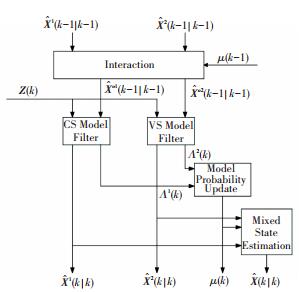 Figure 2 IMM-CCKF (one cycle)
 where
$\left\{ \begin{array}{l}\mathit{\boldsymbol{\nu }}_k^j = \mathit{\boldsymbol{Z}}\left( k \right) - {\mathit{\boldsymbol{H}}^j}\left( k \right){{\mathit{\boldsymbol{\hat X}}}^j}\left( {k\left| {k - 1} \right.} \right)\\\mathit{\boldsymbol{S}}_k^j = {\mathit{\boldsymbol{H}}^j}\left( k \right){\mathit{\boldsymbol{P}}^j}\left( {k\left| {k - 1} \right.} \right){\mathit{\boldsymbol{H}}^j}{\left( k \right)^\prime } + \mathit{\boldsymbol{R}}\left( k \right)\end{array} \right.$ (21)
Using the likelihood evaluated in Eq.(20), we can update the mode probability μ(k). Finally, the estimates of two filters are combined to find the overall estimate
In this cycle, UKF is introduced to obtain
3 Simulation ResultsSimulations and performance comparisons are presented in this section to evaluate the effectiveness of the proposed models and methods.
Firstly, a simple scenario, the nearly constant speed motion with linear equality constraint, is considered. The previously published methods, such as MRKF[4-6], EPKF[7-8], PMKF[9-10] and LECKF[11-12] are claimed to be able to deal with this case. Comprehensive comparisons of the proposed CCKF with the new initialization method against the methods mentioned above are presented in this case. Numerical results show the superiority of the CCKF and the effectiveness of the new initialization method.
A complex motion, switching between the nearly constant speed and the nearly constant acceleration model with a circular nonlinear equality constraint is then explored to illustrate the effectiveness of the proposed IMM-CCKF method. Due to the dependence between shape of trajectory and motion model, the four existing methods mentioned above all loss ability to provide proper estimation.
3.1 Scenario with Linear ConstraintThe target is assumed to move along a linear segment with a constant speed of 50 m/s. In this case, the width of the road is assumed to be comparable to the measurement error so that it can be ignored and we can regard the target as a point.
This segment starts from (200 m, 300 m). The linear equality constraint can be expressed by:
$\mathit{\boldsymbol{C}}{\mathit{\boldsymbol{x}}_k} = d$ (22)
where xk=[xk yk ?k ?k], C=[0 0 1-tan θ′], d=0 and θ′=36.87°.
All the filters are initialized by the first two measurements. The process noise standard deviations are set as 0.005 m/s2 while the measurement error standard deviations are 5 m. The sampling interval is T=1 s. Simulations are performed over 1 000 Monte Carlo runs.
We use absolute and relative root mean squared error (RMSE) of target's position as metrics to distinguish the performances of the constraint estimation methods.
${\rm{relative}}\;\;{\rm{RMSE = }}\frac{{{\rm{RMSE}}\;\;{\rm{of}}\;\;{\rm{constrained}}\;\;{\rm{Kalman}}\;\;{\rm{filter}}}}{{{\rm{RMSE}}\;\;{\rm{of}}\;\;{\rm{unconstrained}}\;\;{\rm{Kalman}}\;\;{\rm{filter}}}}$
Figs. 3 and 4 show the estimation performance of all five constrainted estimation methods. It can be easily seen that the performance can be divided into three levels, the PMKF and EPKF as the worst level, the LECKF and MRKF as the middle level and the CCKF as the best level. The error curves of the filters using the pseudo measurement method and the projection method overlap with each other. That means they have the same performance in this case. Besides, the filters using the model reduction method and the linear equality constraint Kalman filter method perform better than those two methods. It can be also seen that the CCKF outperforms the other four obviously during all the filtering stages.
Figure 3
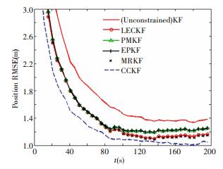 Figure 3 Position RMSE comparison
 Figure 4
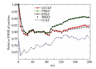 Figure 4 Relative position RMSE comparison
 Also, the performances of the joint initialization in two-dimension and the simple initialization in one-dimension of CCKF are compared as shown in Fig. 5. It can be easily seen that joint initialization as introduced in section 2.2 does improve the performance in initial stage of filtering process since it adopts minimum mean square error fusion method to reduce the error.
Figure 5
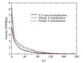 Figure 5 Initialization comparison of CCKF
 Finally, the computational load is explored. We use the ratio between unconstrained KF (UCKF) and other filters as the metric. All the filters are performed on the same desktop computer by MATLAB. As shown in Table 1, the processing time spent by RCKF is smaller than that of MRKF and LECKF but larger compared to that of PMKF and EPKF. Considering the outstanding performance of CCKF, this computational efficiency is acceptable.
表 1
Ratio 1.0 1.3 1.3 2.2 2.3 3.0
Table 1 Relative computational load
3.2 Scenario with Complex MotionThen, we take a circle segment as an example in order to show the performance of IMM-CCKF in tracking ground target with nonlinear constraint and complicated motion. The trajectory, starting from (10 000 m, 3 000 m) with the radius of 5 000 m and the center at (6 000 m, 6 000 m), is shown in Fig. 6 as well as the measurements and the estimates.
Figure 6
 Figure 6 Trajectory with nonlinear constraint
 The target is assumed to travel at a speed of 50 m/s in 0-100 s and there is an acceleration of 0.5 m/s2 in the period of 100-200 s. After that, the speed keep constant again during 200-300 s and in 300-400 s there is a deceleration of 0.5 m/s2.
Two algorithms are taken as contrasts to the proposed IMM-CCKF method: (1) The IMM filter working in the two-dimensional Cartesian state space with constant velocity (CV) and constant acceleration (CA) models (IMM-CVCA); (2) The IMM filter working in the two-dimensional Cartesian state space with CV, CA and CT models (IMM-CVCACT). All the filters are initialized by the first two measurements. The process noise standard deviations are set as 0.005 m/s2 and the measurement error standard deviations as 5 m. The sampling interval is T=5 s. Simulations are performed over 1 000 Monte Carlo runs. The model transition probability matrix of IMM-CCKF is designed as:
$\left[ {\begin{array}{*{20}{c}}{0.85}&{0.15}\\{0.15}&{0.85}\end{array}} \right]$
And the probability matrix of the IMM-CVCACT is designed as:
$\left[ {\begin{array}{*{20}{c}}{0.90}&{0.05}&{0.05}\\{0.05}&{0.90}&{0.05}\\{0.05}&{0.05}&{0.90}\end{array}} \right]$
The root mean squared error (RMSE) of target's position and velocity are used as metrics to distinguish the performances of the maneuvering target tracking methods.
Figs. 7 and 8 show the comparison of IMM-CCKF with the two algorithms. Obvious results can be seen that IMM-CCKF brings better filtering accuracy. When the target enters acceleration stage, the other two IMM algorithms show divergence in different degrees due to the model mismatch.
Figure 7
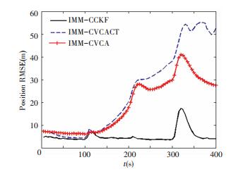 Figure 7 Position RMSE comparison of IMM-CCKF
 Figure 8
 Figure 8 Velocity RMSE comparison of IMM-CCKF
 The model probabilities of IMM-CCKF are shown in Fig. 9. It shows that two models work properly in the IMM-CCKF algorithm. When the target is moving forward at a constant speed in the first 100 s and 200-300 s, the model probability of the CS model is higher than that of VS model. Also we can see in 100-200 s and 300-400 s, the VS model has a higher probability than the CS model due to the acceleration in these periods.
Figure 9
 Figure 9 Model probabilities of IMM-CCKF
 4 ConclusionsThis paper deals with the motion modeling and tracking in road coordinates. An improved initialization method, which uses the optimal fusion of the position measurements in different directions, was presented for the constraint coordinate Kalman filter (CCKF). The nearly constant speed (CS) and varying speed (VS) models in constraint coordinates were used to express complex motions on roads and the corresponding IMM-CCKF was proposed. Simulation results demonstrated the outperformance of the CCKF over the state-of-art linear equality constraint estimation methods due to the modified initialization and more reasonable motion models. The effectiveness of the IMM-CCKF in complex motion modeling and state estimation was also illustrated by numerical experiments.
References
[1]Julier S J, LaViola J J. On Kalman filtering with nonlinear equality constraints.IEEE Transactions on Signal Processing, 2007, 55(6): 2774-2784.DOI:10.1109/TSP.2007.893949(
 0)
0)[2]Pizzinga A. Further investigation into restricted Kalman filtering.Statistics and Probability Letters, 2009, 79(2): 264-269.DOI:10.1016/j.spl.2008.08.005(
 0)
0)[3]Simon D. Kalman filtering with state constraints: A survey of linear and nonlinear algorithms.IET Control Theory and Applications, 2010, 4(8): 1303-1318.DOI:10.1049/iet-cta.2009.0032(
 0)
0)[4]Hemami H, Wyman B. Modeling and control of constrained dynamic systems with application to biped locomotion in the frontal plane.IEEE Transactions on Automatic Control, 1979, 24(4): 526-535.DOI:10.1109/TAC.1979.1102105(
 0)
0)[5]Pizzinga A. Constrained Kalman filtering: Additional results.International Statistical Review, 2010, 78(2): 189-208.DOI:10.1111/j.1751-5823.2010.00098.x(
 0)
0)[6] Wen W, Durrant-Whyte H F. Model-based multi-sensor data fusion. Proceedings of IEEE International Conference on Robotics and Automation, Piscataway:IEEE, 1992.1720-1726. (
 0)
0)[7]Doran H E. Constraining Kalman filter and smoothing estimates to satisfy time-varying restrictions.Review of Economic and Statistics, 1992, 74(3): 568-572.DOI:10.2307/2109505(
 0)
0)[8]Tahk M, Speyer J L. Target tracking problems subject to kinematic constraints.IEEE Transactions on Automatic Control, 1990, 35(3): 324-326.DOI:10.1109/9.50348(
 0)
0)[9]Simon D, Chia T L. Kalman filtering with state equality constraints.IEEE Transactions on Aerospace and Electronic Systems, 2002, 38(1): 128-136.DOI:10.1109/7.993234(
 0)
0)[10]Yang C, Blasch E. Kalman filtering with nonlinear state constraints.IEEE Transactions on Aerospace and Electronic Systems, 2009, 45(1): 70-84.DOI:10.1109/TAES.2009.4805264(
 0)
0)[11]Ko S, Bitmead R. State estimation for linear systems with state equality constraints.Automatica, 2007, 43(8): 1363-1368.DOI:10.1016/j.automatica.2007.01.017(
 0)
0)[12]Xu L, Li X R, Duan Z, et al. Modeling and state estimation for dynamic systems with linear equality constraints.IEEE Transactions on Signal Process, 2013, 61(11): 2927-2939.DOI:10.1109/TSP.2013.2255045(
 0)
0)[13] Duan Z, Li X R. Constrained target motion modeling-part I: Straight line track. Proceedings of the 16th International Conference on Information Fusion, Istanbul, 2013.2153-2160. (
 0)
0)[14]Hewett R J, Health M T, Butala M D, et al. A robust null space method for linear equality constrained state estimation.IEEE Transactions on Signal Processing, 2010, 58: 3961-3971.DOI:10.1109/TSP.2010.2048901(
 0)
0)[15] Duan Z, Li X R. Constrained target motion modeling-Part II: Circular track. Proceedings of the 16th International Conference on Information Fusion, Istanbul, 2013.2161-2167. (
 0)
0)[16] Duan Z, Li X R, Ru J F. Design and analysis of linear equality constrained dynamic systems. Proceedings of the 15th International Conference on Information Fusion, Singapore, 2012.2537-2544. (
 0)
0)[17] Yang C, Bakich M, Blasch E. Nonlinear constrained tracking of targets on roads. Proceedings of the 8th International Conference on Information Fusion, Philadelphia, PA, 2005. 235-242. (
 0)
0)[18]Ulmke M, Koch W. Road-map assisted ground moving target tracking.IEEE Transactions on Aerospace and Electronic Systems, 2006, 42(4): 1264-1274.DOI:10.1109/TAES.2006.314571(
 0)
0)[19]Kirubarajan T, Bar-Shalom Y, Pattipati K R, et al. Ground target tracking with variable structure IMM estimator.IEEE Transactions on Aerospace and Electronic Systems, 2000, 36(1): 26-46.DOI:10.1109/7.826310(
 0)
0)[20] Koch W. GMTI-tracking and information fusion for ground surveillance. Proceedings of SPIE, 2001.381-392. DOI:10.1117/12.492764. (
 0)
0)[21] Bar-Shalom Y, Li X R, Kirubarajan T. Estimation with Applications to Tracking and Navigation: Theory, Algorithms, and Software. New York: Wiley, 2001.453-457. (
 0)
0)[22] Bar-Shalom Y, Willett P K, Tian X. Tracking and Data Fusion: A Handbook of Algorithms, Storrs, CT: YBS Publishing, 2011. (
 0)
0)[23]Blom H A P, Bar-Shalom Y. The interacting multiple model algorithm for systems with markovian switching coefficients.IEEE Transactions on Automatic Control, 1988, 33(8): 780-783.DOI:10.1109/9.1299(
 0)
0)[24] Zhang M, Knedlik S, Loffeld O. An adaptive road-constrained IMM estimator for ground target tracking in GSM networks. Proceedings of the 11th International Conference on Information Fusion, Cologne, 2008.1-8. (
 0)
0)[25]Julier S J, Uhlmann J, Durrant-Whyte H F. A new method for the nonlinear transformation of means and covariances in filters and estimators.IEEE Transactions on Automatic Control, 2003, 45(3): 477-482.(
 0)
0)