Tie Gang1, Yilin Luan2, Chi Zhang1
(1. State Key Laboratory of Advanced Welding and Joining, Harbin Institute of Technology, Harbin 150001, China;2. School of Materials Science and Engineering, Heilongjiang University of Science and Technology, Harbin 150022, China)
Abstract:
A feature extraction method was proposed to sectorial scan image of Ti-6Al-4V electron beam welding seam based on principal component analysis to solve problem of high-dimensional data resulting in time-consuming in defect recognition. Seven features were extracted from the image and represented 87.3 % information of the original data. Both the extracted features and the original data were used to train support vector machine model to assess the feature extraction performance in two aspects: recognition accuracy and training time. The results show that using the extracted features the recognition accuracy of pore, crack, lack of fusion and lack of penetration are 93%, 90.7%, 94.7% and 89.3%, respectively, which is slightly higher than those using the original data. The training time of the models using the extracted features is extremely reduced comparing with those using the original data.
Key words: electron beam welding phased array ultrasonic sectorial scan image feature extraction principal component analysis
DOI:10.11916/j.issn.1005-9113.15287
Clc Number:TG115.28
Fund:
Tie Gang, Yilin Luan, Chi Zhang. Feature Extraction of Sectorial Scan Image of Thick-Walled Electron Beam Welding Seam Based on Principal Component Analysis[J]. Journal of Harbin Institute of Technology, 2017, 24(6): 45-51. DOI: 10.11916/j.issn.1005-9113.15287.

Fund Sponsored by the National Natural Science Foundation of China (Grant Nos.51575134 and 51205083) Corresponding author Yilin Luan, E-mail: ylluan@hit.edu.cn Article history Received: 2015-12-12
Contents Abstract Full text Figures/Tables PDF
Feature Extraction of Sectorial Scan Image of Thick-Walled Electron Beam Welding Seam Based on Principal Component Analysis
Tie Gang1, Yilin Luan2

 , Chi Zhang1
 1. State Key Laboratory of Advanced Welding and Joining, Harbin Institute of Technology, Harbin 150001, China;
2. School of Materials Science and Engineering, Heilongjiang University of Science and Technology, Harbin 150022, China
Received: 2015-12-12
Fund: Sponsored by the National Natural Science Foundation of China (Grant Nos.51575134 and 51205083)
Corresponding author: Yilin Luan, E-mail: ylluan@hit.edu.cn
Abstract: A feature extraction method was proposed to sectorial scan image of Ti-6Al-4V electron beam welding seam based on principal component analysis to solve problem of high-dimensional data resulting in time-consuming in defect recognition. Seven features were extracted from the image and represented 87.3 % information of the original data. Both the extracted features and the original data were used to train support vector machine model to assess the feature extraction performance in two aspects: recognition accuracy and training time. The results show that using the extracted features the recognition accuracy of pore, crack, lack of fusion and lack of penetration are 93%, 90.7%, 94.7% and 89.3%, respectively, which is slightly higher than those using the original data. The training time of the models using the extracted features is extremely reduced comparing with those using the original data.
Key words: electron beam welding phased array ultrasonic sectorial scan image feature extraction principal component analysis
1 Introduction In recent years, electron beam welding has been widely used in the field of thick-walled structures. Narrow heat affected zone, minimal distortion and rapid production time are obtained by this joining process when compares to conventional welding techniques[1-2]. Mechanical properties of welding seam are strongly influenced by welding quality[3-4]. Defects in different sizes and concentrations can significantly degrade strength and service performance of welding structures. Thus it is necessary to accurately evaluate quality of electron beam welding seam[5].
Conventional ultrasonic inspection usually uses a single-element probe which must be moved to sweep the beam through the whole welding seam. It has limited detection capability if a thick-walled welding structure has restricted space to move a probe. An advanced ultrasonic testing method, phased array ultrasonic, can resolve this problem. Phased array ultrasonic is based on the use of probe made up of individual elements that can each be independently driven and enable simultaneous or different emission and reception[6-7]. The beam from a phased array probe can be moved electronically without moving the probe, and can sweep through an angular range for a specific depth, which is called phased array sectorial scan[8].
In the following feature extraction procedure, choosing informative, discriminating and independent features is a crucial step for effective defect recognition algorithms[9]. Phased array sectorial scan makes welding inspection feasible and convenient than ever before. At the same time, it receives a large number of data, which make feature extraction complex. Some feature extraction methods have been performed on sectorial scan images, such as fractal-based feature extraction[10], texture feature extraction[11], and lifted wavelet transform[12]. These feature extraction methods extract informative features to a certain extent, but do not significantly reduce the dimensions of the data. This causes many problems. Algorithms that operate on high-dimensional data tend to be time-consuming. Many machine learning algorithms struggle with high-dimensional data[13]. Reducing high-dimensional data into low dimensions often makes machine learning algorithms more efficient and more accurate. Principal component analysis uses an orthogonal transformation to convert a set of correlated variables into a set of uncorrelated variables called principal components. The number of principal components is usually less than the number of original variables.
In this paper, a novel feature extraction method is proposed to phase array sectorial scan image of Ti-6Al-4V electron beam welding seam. The method is based on principal component analysis to extract linearly uncorrelated features from the original data. The aim of the study is not only to extract informative features that can contribute to classification, but to save time of defect recognition algorithms. The authors shall demonstrate the effectiveness in classification time saving of the method.
2 Experimental Methods 2.1 Specimens The material used in this study was Ti-6Al-4V alloy. The nominal composition of the alloy in weight percent is: Al, 5.8; V, 4.0; Fe, 0.3; O, 0.1; C, 0.08; N, 0.05; H, 0.015 and the balance Ti. The welding specimens were machined to a rectangular shape of 255 mm × 65 mm, and the thickness was 55 mm. The electron beam welding was performed in a Medard45 electron beam welding machine under the conditions of a beam current of 200 mA, an accelerating voltage of 70 kV, a convergent current of 773 mA.
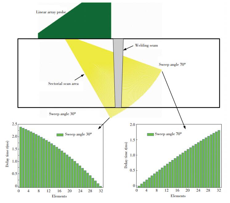
2.2 Phased Array Sectorial Scan Phased array sectorial scan was performed using a X-32 phased array testing system. A linear array probe with 32 elements and central frequency at 5 MHz was used. The elements were in a rectangular shape of 0.8 mm×12 mm and the gap between the elements was 0.04 mm. The material of the wedge was acryl glass and the angle of the wedge was 35°. The focal distance was 70 mm to guarantee the beam to sweep through the whole seam. The sweep angles varied from 30° to 70° with a step of 0.5°. The delay time of each element was calculated by the phased array testing system. The diagrammatic sketch of the sectorial scan and examples of the delay time were illustrated in Fig. 1.
Figure 1
 Figure 1 Diagrammatic sketch of the sectorial scan and examples of the delay time
 2.3 Metallographic Analysis The specimens were cut after ultrasonic testing and the cross sections of Ti-6Al-4V electron beam welding seam were prepared by standard polishing techniques. The microstructures of the welding seam were examined by an optical SZX12 microscope.
3 Feature Extraction The feature extraction of the sectorial scan images was performed based on principal component analysis. The first principal component has the largest possible variance which accounts for as much of the variability in the data as possible and each succeeding component in turn has the highest variance under the constraint that it is orthogonal to the preceding components[14]. This was why principal component analysis was chosen for the feature extraction. The procedures of the feature extraction using covariance method were as follows:
(1) Organised the data of the sectorial scan images of the defects.
Collected the sectorial scan images of the defects. Four kinds of defects were observed in Ti-6Al-4V electron beam welding seam. They were pore, crack, lack of fusion and lack of penetration. The number of the sectorial scan images for each kind of the defect were 720, 947, 813 and 952, respectively. The total number of the sectorial scan images was 3 432. A sectorial scan image comprised 81 A-scan signals and each A-scan signal comprised 720 variables. Therefore, each sectorial scan image consisted of 720×81=58 320 variables. The data of the sectorial scan images were arranged as a set of row vectors X1, X2, …, X3 432 with each Xi representing a single sectorial scan image of 58 320 variables. Placed the row vectors into a single matrix X of dimensions 3 432×58 320.
(2) Calculated the empirical mean of the matrix X.
Found the empirical mean along each dimension j=1, 2, ……, 58 320. Placed the calculated mean values into an empirical mean vector m of dimensions 1×58 320.
$\mathit{\boldsymbol{m}}\left( j \right) = \frac{1}{{3432}}\sum\limits_{i = 1}^{3432} {\mathit{\boldsymbol{X}}\left[ {i,j} \right]} $
(3) Calculated the deviations from the mean.
Subtracted the empirical mean vector m from each row of the data matrix X. Stored the mean subtracted data in the 3 432×58 320 matrix B.
$\mathit{\boldsymbol{B}} = \mathit{\boldsymbol{X}} - \mathit{\boldsymbol{hm}}$
where h was an 3 432×1 column vector of all ones.
(4) Found the covariance matrix.
Found the 58 320×58 320 covariance matrix Σ from the outer product of the matrix B with itself:
$\mathit{\boldsymbol{ \boldsymbol{\varSigma} = }}\frac{1}{{3432 - 1}}{\mathit{\boldsymbol{B}}^ * } \cdot \mathit{\boldsymbol{B}}$
where * was the conjugate transpose operator.
(5) Found the eigenvalues and the eigenvectors of the covariance matrix.
Computed the eigenvector matrix V,
${\mathit{\boldsymbol{V}}^{ - 1}}\mathit{\boldsymbol{ \boldsymbol{\varSigma} V}} = \mathit{\boldsymbol{D}}$
where matrix D was an 58 320×58 320 diagonal matrix,
$\mathit{\boldsymbol{D}}\left[ {i,j} \right] = \left\{ \begin{array}{l}{\lambda _i},\;\;\;\;\;\;i = j\\0,\;\;\;\;\;\;\;i \ne j\end{array} \right.$
where λi was the ith eigenvalue of the covariance matrix Σ.
The matrix V, with dimensions of 58 320×58 320, contained 58 320 column vectors, which represented the 58 320 eigenvectors of the covariance matrix Σ. Sorted the columns of the eigenvector matrix V and the eigenvalue matrix D in order of decreasing eigenvalue.
(6) Computed the cumulative energy content for each eigenvector.
The eigenvalues represented the distribution of the data's energy among each of the eigenvector, where the total eigenvectors formed a basis for the data. The cumulative energy content g for the kth eigenvector was the sum of the energy content across all of the eigenvalues from 1 through k:
$g\left( k \right) = \sum\limits_{i = 1}^k {{\lambda _i}\;} {\rm{for}}\;k = 1,2, \cdots \cdots ,58320$
(7) Selected a subset of the eigenvectors.
Chose a value of K (for 1≤K≤58 320) as small as possible while achieving a reasonably high value of g on a percentage basis. In this study, chose the smallest value of K such that:
$\frac{{g\left( K \right)}}{{g\left( {58320} \right)}} \times 100\% \ge 85\% $ (1)
Saved the first K columns of V as the 58 320×K matrix W:
$\begin{array}{l}\mathit{\boldsymbol{W}}\left[ {i,j} \right] = \mathit{\boldsymbol{V}}\left[ {i,j} \right]\;{\rm{for}}\;i = 1,2, \cdots \cdots ,58320,\\\;\;\;\;\;\;\;\;\;\;\;\;\;\;j = 1,2, \cdots ,K\end{array}$
(8) Extracted the features of the sectorial scan images.
Calculated the feature matrix F of dimensions 3 432×K:
$\mathit{\boldsymbol{F}} = \mathit{\boldsymbol{B}} \cdot \mathit{\boldsymbol{W}}$ (2)
The feature matrix F contained K column vectors F1, F2, …, FK. Each Fj of dimensions 3 432×1 represented a feature of the sectorial scan images. Fij was the jth feature of the ith sectorial scan image (for i=1, 2, …, 3 432, j=1, 2, …, K).
4 Defect Recognition The Defect recognition, which was performed using support vector machine (SVM), followed the feature extraction. SVM is a supervised learning model to construct an optimal hyperplane as the decision surface that the margin of separation between the closest data points belonging to two categories is maximised. For a binary classification problem, given a set of training data, each marked for belonging to one of two categories, a SVM training algorithm builds a model that assigns new data into one category or the other[15].
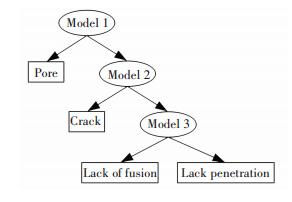
A binary decision tree was used for multi-category classification problem. A SVM in each node of the tree is trained using two of the categories. Considering the distinction of the four kinds of defects, the architecture of the binary decision tree was carefully designed as shown in Fig. 2. Three models needed to be trained by utilizing this architecture. The first model was trained to separate the pores from the other three kinds of defects. The pores were considered as one category and the other three kinds of defects were considered as the other category. In the similar way, the second model was trained to recognise the cracks from the lack of fusions and the lack of penetrations. The cracks were considered as one category and the lack of fusions and the lack of penetrations were considered as the other category. The third model was trained to distinguish the lack of fusions from the lack of penetrations.
Figure 2
 Figure 2 Architecture of the binary decision tree for the defect recognition
 It often happens that the data are not linearly separable in that space. To solve the problem, the original finite-dimension space should be mapped into a much higher-dimensional space by applying a kernel function[16]. The radial basis function kernel was chosen in the recognition:
$K\left( {x,y} \right) = \exp \left( { - \gamma {{\left\| {x - y} \right\|}^2}} \right)$
where γ was kernel parameter.
The following procedures were utilised during the training stage:
1) Prepared the training and the testing set. The data instances were selected randomly from the feature matrix. For each kind of the defect, the number of the data instances was 500. A 40% of the data instances were set aside as the training set and the remaining 60% of the data instances were used as the testing set. Note that the training and the testing set were different for different models.
2) Determined parameter C and γ (Parameter C is a user specified positive value that controls the trade-off between maximizing the margin and minimizing the error). Grid search method was used to estimate accuracy for all possible combinations of C and γ.
3) Trained the model using the determined C and γ values.
Three models were trained according to the above procedures. Then the testing set was input to the binary decision tree. The recognition started at the root of the tree. At each node of the binary tree a decision was made by transferring the testing datum to the left node or to the right sub-tree. This was repeated recursively downward the tree until the datum reached a leaf node that represented the category it has been assigned to. The recognition accuracy RA for each kind of the defect was evaluated by:
${R_A} = \frac{{{N_r}}}{{{N_t}}} \times 100\% $ (3)
where Nr was the number of the testing set that had been correctly recognised and Nt was the total number of the testing set. Note that the recognition accuracy for the four kinds of defects should be calculated separately.
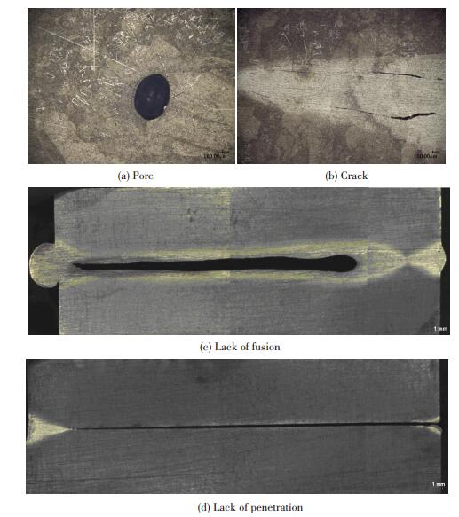
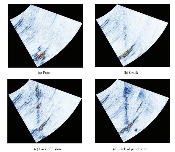
5 Results and Discussion Fig. 3 shows the typical microstructures of the pore, the crack, the lack of fusion and the lack of penetration which were observed in Ti-6Al-4V electron beam welding seam. Corresponding phased array sectorial scan images of the defects are shown in Fig. 4. Relationship between the defects and the sectorial scan images was built for further feature extraction analysis.
Figure 3
 Figure 3 Metallograph of the defects in Ti-6Al-4V electron beam welding seam
 Figure 4
 Figure 4 Sectorial scan images of the defects in Ti-6Al-4V electron beam welding seam
 The calculated covariance matrix Σ of the data matrix X is:
$\mathit{\boldsymbol{ \boldsymbol{\varSigma} }} = \left[ {\begin{array}{*{20}{c}}{0.404}&{0.404}& \cdots &{0.294}\\{0.404}&{0.591}& \cdots &{0.390}\\ \vdots&\vdots&\vdots&\vdots \\{0.294}&{0.390}& \cdots &{0.432}\end{array}} \right]$
The rearranged eigenvalue matrix D in order of decreasing eigenvalue is:
$\mathit{\boldsymbol{D}} = \left[ {\begin{array}{*{20}{c}}{31.1}&0& \cdots &0\\0&{4.5}& \cdots &0\\ \vdots&\vdots&\vdots&\vdots \\0&0& \cdots &{0.00001}\end{array}} \right]$
The smallest value of K was chosen according to Eq.(1). Table 1 shows the eigenvalues, the cumulative energy contents g and the g on a percentage basis. As can be seen from the table, the g on a percentage basis is achieved a value of 87.3% which is higher than 85% when K equals 7.
表 1
λ1 31.1 g(1) 31.1 57.9
λ2 4.5 g(2) 35.6 66.2
λ3 2.9 g(3) 38.5 71.5
λ4 2.7 g(4) 41.2 76.5
λ5 2.4 g(5) 43.6 80.9
λ6 1.9 g(6) 45.5 84.4
λ7 1.6 g(7) 47.1 87.3
Table 1 The eigenvalues and the cumulative energy contents
Then subset matrix W with dimensions of 7×58 320 is:
$\mathit{\boldsymbol{W}} = \left[ {\begin{array}{*{20}{c}}{ - 0.252}&{ - 0.418}&{ - 0.199}&{0.233}&{ - 0.091}&{ - 0.048}&{ - 0.063}\\{ - 0.357}&{ - 0.112}&{0.149}&{0.596}&{0.550}&{ - 0.393}&{ - 0.017}\\ \vdots&\vdots&\vdots&\vdots&\vdots&\vdots&\vdots \\{ - 0.311}&{0.007}&{ - 0.263}&{0.068}&{ - 0.027}&{ - 0.057}&{ - 0.053}\end{array}} \right]$
The feature matrix F obtained by Eq.(2) was:
$\mathit{\boldsymbol{F}} = \left[ {\begin{array}{*{20}{c}}{0.173}&{0.515}&{0.855}&{0.309}&{0.352}&{0.142}&{0.512}\\{0.919}&{0.139}&{0.405}&{0.640}&{0.671}&{0.188}&{0.029}\\ \vdots&\vdots&\vdots&\vdots&\vdots&\vdots&\vdots \\{0.512}&{0.724}&{0.028}&{0.435}&{0.468}&{0.957}&{0.410}\end{array}} \right]$
The original data matrix X of dimensions 3 432×58 320 is transformed to the feature matrix F with dimensions of 3 432×7. The feature extraction method significantly reduces the dimensions of the original data. The time consume of the feature extraction is 5.54 s. The purpose of the feature extraction is to choose discriminating features for recognition algorithm. Whether the extracted features can make machine learning algorithm effective or not, the following recognition results give the answer.
Three defect recognition models are shown in Fig. 5. Symbols '○' and '△' represent two different categories. Note that symbols in different models have different meanings. The hyperplane is a 6-dimensional space, which is only given the projection in the plane of feature F1 and feature F2. It separates the space into two half spaces. The recognition results estimated by Eq.(3) show that recognition accuracy of the pore, the crack, the lack of fusion and the lack of penetration are 93.3 %, 90.7 %, 94.7 % and 89.3 %, respectively. It can be seen that these four kinds of defects are successfully recognised. That means the extracted features are effective in the SVM algorithm.
Figure 5
 Figure 5 Recognition models
 The defect recognition using the original data of sectorial scan image was also performed using the same method mentioned in Section 4 for comparison in training time and recognition accuracy with the feature extraction method. Table 2 shows the training time of two kinds of recognition models. It can be seen that the training time of the models using the extracted features are extremely decreased comparing with those of using the original data. The feature extraction method solves the time-consuming problem which often occurs in high-dimensional data learning algorithms. Recognition accuracy comparison is shown in Table 3. The algorithm that operates on the extracted feature obtains slightly higher accuracy than that operates on the original data.
表 2
Model 1 9.41 184.76
Model 2 7.83 156.37
Model 3 6.45 134.89
Table 2 Training time comparison
表 3
pore 93.3 91.3
crack 90.7 89.3
lack of fusion 94.7 92.7
lack of penetration 89.3 88.7
Table 3 Recognition accuracy comparison
6 Conclusions From the above study we may reasonably arrive at the conclusion that the features of the defects in Ti-6Al-4V electron beam welding seam are extracted successfully from the sectorial scan image using the proposed algorithm. The extracted seven features represent 87.3% information of the original data, which are contributive to defect classification. The recognition accuracy of the pore, the crack, the lack of fusion and the lack of penetration are 93.3%, 90.7%, 94.7% and 89.3%, respectively. It also significantly decreases training time of the recognition model. The phased array ultrasonic is applied not only to welding seam but to many other fields, such as casting and adhesive structure. The algorithm shall be applied to other sectorial scan inspections to analyse its universal ability in our further study.
AcknowledgementThe authors are grateful to all the members of nondestructive testing research team of State Key Laboratory of Advanced Welding and Joining in Harbin Institute of Technology for their helps.
References
[1] Vráblík F, Clau U, Stolar P. Electron beam welding-A key technology to construct vehicles for road, rail, sea, air and space. Proceedings of 19th International Conference on Metallurgy and Materials. Roznov pod Radhostem: TANGER Ltd., 2010. 590-595. (
 0)
0)[2] AyresK R, Hurrell P R, Gill C M, et al. Development of reduced pressure electron beam welding process for thick section pressure vessel welds. American Society of Mechanical Engineers, Pressure Vessels and Piping Division (Publication) PVP. Washington, 2010, 6: 39-48. DOI: 10.1115/PVP2010-25957. (
 0)
0)[3] Reimche W, Bach F W, Mroz G, et al. High strength 3D non-vacuum electron beam weld joints-setting of gradient material properties and testing of weld quality. Steel Research International, 2008, 79(3): 225-232. DOI:10.1002/srin.2008.79.issue-3 (
 0)
0)[4] Neuenschwander J, Blau B, Christin R, et al. Quality monitoring of the electron beam welding of the CMS conductor using ultrasonics. IEEE Transactions on Applied Superconductivity, 2014, 14(2): 526-529. DOI:10.1109/TASC.2004.829711 (
 0)
0)[5] Zhou Q, Liu F J, Li Z J, et al. Application of ultrasonic phased array imaging in electron beam welding inspection. China Welding, 2002, 11(2): 114-118. (
 0)
0)[6] Waters C. Phased array ultrasonic inspection of welds -A new solution. Materials Forum, 2006, 30: 45-48. (
 0)
0)[7] Miki M, Ogata M. Phased array ultrasonic testing methods for welds in bogie frames of railway vehicles. Insight Non-Destr. Test Cond. Monit, 2015, 57: 382-388. DOI:10.1784/insi.2015.57.7.382 (
 0)
0)[8] Lozev M G, Shell E B, Spencer R L, et al. Testing superaustenitic stainless steel welds using phased array ultrasonics. Materials Evaluation, 2004, 62(11): 1135-1141. (
 0)
0)[9] Lampinen J, Smolander S. Self-organizing feature extraction in recognition of wood surface defects and color images. International Journal of Pattern Recognition and Artificial Intelligence, 1996, 10(2): 97-113. DOI:10.1142/S0218001496000098 (
 0)
0)[10] Zhan X L, Jin S J. A fractal-based flaw feature extraction method for ultrasonic phased array nondestructive testing. Proceedings of IEEE International Conference on Mechatronics and Automation. Piscataway: IEEE Computer Society, 2009. 1606-1611. DOI: 10.1109/ICMA.2009.5246076. (
 0)
0)[11] Yang X X, Chen S L, Jin S J, et al. Crack orientation and depth estimation in a low-pressure turbine disc using a phased array ultrasonic transducer and an artificial neural network. Sensors, 2013, 13(9): 12375-12391. DOI:10.3390/s130912375 (
 0)
0)[12] Li J, Zhan X L, Jin S J. New flaw feature extraction method for ultrasonic phased array nondestructive testing. Proceedings of 8th International Conference on Intelligent Control and Automation. Piscataway: Institute of Electrical and Electronics Engineers Inc., 2010. 6998-7003. DOI: 10.1109/WCICA.2010.5554254. (
 0)
0)[13] Choi J Y, Bae S H, Qiu X H, et al. High performance dimension reduction and visualization for large high-dimensional data analysis. Proceedings of IEEE/ACM International Symposium on Cluster, Cloud, and Grid Computing. Piscataway: IEEE Computer Society, 2010. 331-340. DOI: 10.1109/CCGRID.2010.104. (
 0)
0)[14] Jolliffe I T. Principal Component Analysis. New York: Springer, 2002, 28-40. (
 0)
0)[15] Vapnik V N. The Nature of Statistical Learning Theory. New York: Springer, 2000, 138-146. (
 0)
0)[16] Boser B E, Guyon I M, Vapnik V N. A training algorithm for optimal margin classifiers. Proceedings of 5th International Conference on Computational learning theory. New York: ACM Press, 1992. 144-152. (
 0)
0)