Small phenomenology on gluon evolution through the BFKL equation in light of a constraint in multi-
本站小编 Free考研考试/2022-01-02
Pragyan Phukan,, Madhurjya Lalung,, Jayanta Kumar Sarma,1HEP laboratory, Department of Physics, Tezpur University, India
First author contact:1 Author to whom any correspondence should be addressed. Received:2019-10-9Revised:2019-11-10Accepted:2019-11-26Online:2020-02-05
Abstract We investigate the impact of so-called kinematic constraint on gluon evolution at small x. Implanting the constraint on the real emission term of the gluon ladder diagram, we obtain an integro-differential form of the Balitsky-Fadin-Kuraev-Lipatov (BFKL) equation. Later we solve the equation analytically using the method of characteristics. We sketch the Bjorken x and transverse momentum ${k}_{t}^{2}$ dependence of our solution of unintegrated gluon distributions $f(x,{k}_{t}^{2})$ in the kinematic constraint supplemented BFKL equation and contrasted the same with the original BFKL equation. Then we extract the integrated gluon density xg(x, Q2) from unintegrated gluon distributions $f(x,{k}_{t}^{2})$ and compared our theoretical prediction with that of global data fits, namely NNPDF3.1sx and CT14. Finally we illustrate the phenomenological implication of our solution for unintegrated gluon distribution $f(x,{k}_{T}^{2})$ towards exploring high precision HERA DIS data by the theoretical prediction of proton structure functions (F2 and FL). Keywords:parton evolution equation;gluon distribution function;perturbative QCD
PDF (1022KB)MetadataMetricsRelated articlesExportEndNote|Ris|BibtexFavorite Cite this article Pragyan Phukan, Madhurjya Lalung, Jayanta Kumar Sarma. Small x phenomenology on gluon evolution through the BFKL equation in light of a constraint in multi-Regge kinematics. Communications in Theoretical Physics, 2020, 72(2): 025201- doi:10.1088/1572-9494/ab61ee
1. Introduction
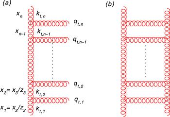
The parton distribution functions (PDFs) serve as a very important tool for the calculation of inclusive cross sections in hadronic collision processes. In perturbative QCD, particularly for moderate values of Bjorken x and large interaction scale Q2, DIS observables are determined by the mass factorization theorem in which the collinear logarithmic singularities arising from gluon splitting are characterized by collinear parton distribution functions. These collinear PDFs are determined by the DGLAP evolution equation [1–6], which resums the leading ${\alpha }_{s}\mathrm{ln}{Q}^{2}$ contributions associated with a space-like chain of n gluons with strongly ordered successive gluon transverse momentum along the chain. On the other hand, at sufficiently high energies ($\sqrt{S}$) or small x, the leading logarithmic contribution of ${\alpha }_{s}\mathrm{ln}(1/x)$ cannot be neglected along the gluon chain. In this regime, the dominant parton is the gluon and the key ingredient to calculate the scattering observables is the unintegrated gluon distributions (ugd’s) entering through kt factorization formula. The ugd’s are characterised by BFKL evolution [7–9], which sums the leading ${\alpha }_{s}\mathrm{ln}(1/x)$ contributions, usually written in the form$\begin{eqnarray}\begin{array}{l}-x\displaystyle \frac{\partial f\left(x,{k}_{t}^{2}\right)}{\partial x}=\displaystyle \frac{{\alpha }_{s}{N}_{c}{k}_{t}^{2}}{\pi }{\displaystyle \int }_{{k}_{0}^{{\prime} 2}}^{\infty }\displaystyle \frac{{{\rm{d}}{k}}_{t}^{{\prime} 2}}{{k}_{t}^{{\prime} 2}}\\ \quad \times \,\left[\displaystyle \frac{f(x,{k}_{t}^{{\prime} 2})-f\left(x,{k}_{t}^{2}\right)}{| {k}_{t}^{{\prime} 2}-{k}_{t}^{2}| }+\displaystyle \frac{f\left(x,{k}_{t}^{2}\right)}{\sqrt{{k}_{t}^{4}+4{k}_{t}^{{\prime} 4}}}\right],\end{array}\end{eqnarray}$where $f\left(x,{k}_{t}^{2}\right)$ denotes the gluon density unintegrated over the gluon transverse momentum kt and ${k}_{0}^{{\prime} 2}$ is the infrared cutoff of the evolution. To gain insight of (1) we refer to figure 1(a), which shows a chain of sequential gluon emission. The BFKL kernel in (1) corresponds to the sum of the gluon ladder diagram in figure 1(b), which is formed by squaring the amplitude of figure 1(a). The real emission is characterized by the first term in the kernel while the second term corresponds to the diagrams with virtual corrections. The apparent singularity observed at ${k}_{t}^{{\prime} 2}={k}_{t}^{2}$ cancels between real and virtual contributions to ensure that there is no overall singularity in (1).
Figure 1.
New window|Download| PPT slide Figure 1.(a) Chain of sequential gluon emission, which forms the basis of the BFKL equation. On squaring the amplitude of (a) the ladder (b) is generated, which, when summed, gives the BFKL kernel.
The real emission term in the BFKL kernel interprets the $k^{\prime} \to k+q$ splitting inside the hadron as shown in figure 1(a). In BFKL multi-regge kinematics the longitudinal component of the gluon momentum is strongly ordered ${x}_{1}\ll {x}_{2}.....\ll {x}_{n-1}\ll {x}_{n}$ whereas there is no ordering in the transverse component ${k}_{1t}\sim {k}_{2t}\sim ....\sim {k}_{{\rm{n}}-1t}\sim {k}_{{\rm{n}}t}$ and the virtuality of the gluon comes dominantly from the transverse component of the momentum i.e.$\begin{eqnarray}{k}^{2}=2{k}^{+}{k}^{-}-{k}_{t}^{2}\approx {k}_{t}^{2}.\end{eqnarray}$As a consequence of these BFKL kinematics, so-called kinematic constraint or consistency constraint comes into the picture and it is implemented in different forms:$\begin{eqnarray}{q}_{t}^{2}\lt \displaystyle \frac{{k}_{t}^{2}}{z}\ \ \ \ \ \ \mathrm{LDC}\ [10,13],\end{eqnarray}$$\begin{eqnarray}{q}_{t}^{2}\lt \displaystyle \frac{(1-z){k}_{t}^{2}}{z}\ \ [14],\end{eqnarray}$$\begin{eqnarray}{k}_{t}^{{\prime} 2}\lt \displaystyle \frac{{k}_{t}^{2}}{z}\ \ \ \ \ \ \ \ \mathrm{BFKL}\ [14,15].\end{eqnarray}$The relation (5) can be considered as a special case of (3) owing to the fact that for a fixed value of kt, a high qt2 would imply an equally high ${k}_{t}^{{\prime} 2}$ [10]. Although other constraints exist as a consequence of energy momentum conservation, this bound is considerably tighter than the latter [10].
Our primary goal of this work is to investigate the effect of this kinematic constraint on the small x regime of gluon evolution. Accordingly, we organise the content of the paper as follows. In section 2.1, we first implemented the kinematic constraint to the ordinary BFKL equation and then solved the kinematic constraint supplemented BFKL equation analytically. We adopt the method of characteristics to solve the PDE. In section 2.2, we built up the theoretical foundation in terms of factorization formula to predict DIS structure functions (F2 and FL). Then in section 3 we present the numerical analysis and portray our results for gluon evolution as well as structure functions. First we sketch both the small x and transverse momentum ${k}_{t}^{2}$ dependence of unintegrated gluon distributions $f(x,{k}_{t}^{2})$. Then we extract integrated gluon density xg(x, Q2) from ugd’s and study x and Q2 dependence of xg(x, Q2). Our theoretical predictions for integrated gluon density xg(x, Q2) is compared with that of global data fits NNPDF3.1sx [12] and CT14 [14]. We also investigate the sensitivity of the BFKL intercept in both x and ${k}_{t}^{2}$ evolution of ugd’s $f(x,{k}_{t}^{2})$. Later we sketched our predictions for DIS structure functions (F2 and FL) and contrasted our results with that of HERA DIS data. Finally in section 4 we summarize and outline our conclusion as well as possible future prospects.
2. Theory
2.1. Formulation and analytical solution of kinematic constrained BFKL
Recall that the BFKL equation can be written as an integral equation for unintegrated gluon distributions $f(x,{k}_{t}^{2})$ in the form [15],$\begin{eqnarray}\begin{array}{rcl}f(x,{k}_{t}^{2}) & = & {f}^{(0)}(x,{k}_{T}^{2})+\displaystyle \frac{{\alpha }_{s}}{2\pi }{\displaystyle \int }_{x}^{1}\displaystyle \frac{{\rm{d}}{z}}{z}\\ & & \times {\displaystyle \int }_{{k}_{0}^{{\prime} 2}}{{\rm{d}}{k}}_{t}^{{\prime} 2}\kappa ({k}^{2},{k}_{t}^{{\prime} 2},z)f\left(\displaystyle \frac{x}{z},{k}_{t}^{{\prime} 2}\right),\end{array}\end{eqnarray}$where the inhomogeneous driving term ${f}^{(0)}(x,{k}_{T}^{2})$ depicts gluon-proton coupling. The BFKL kernel is evaluated as$\begin{eqnarray}\begin{array}{l}\kappa ({k}^{2},{k}_{t}^{{\prime} 2},z)f\left(\displaystyle \frac{x}{z},{k}_{t}^{{\prime} 2}\right)\\ \quad =\,2{N}_{c}\displaystyle \frac{{k}_{t}^{2}}{{k}_{t}^{{\prime} 2}}\left[\displaystyle \frac{{\rm{\Theta }}\left(\tfrac{{k}_{t}^{2}}{z}-{k}_{t}^{{\prime} 2}\right)f\left(\tfrac{x}{z},{k}_{t}^{{\prime} 2}\right)-f\left(\tfrac{x}{z},{k}_{t}^{2}\right)}{\left|{k}_{t}^{{\prime} 2}-{k}_{t}^{2}\right|}\right.\\ \qquad \left.+\,\displaystyle \frac{f\left(\tfrac{x}{z},{k}_{t}^{2}\right)}{\sqrt{{k}_{t}^{4}+4{k}_{t}^{{\prime} 4}}}\right].\end{array}\end{eqnarray}$The so-called kinematic constraint ${k}_{t}^{{\prime} 2}\lt {k}^{2}/z$ is imposed onto the real-emission part of the kernel (7) through the Heaviside theta function ${\rm{\Theta }}\left(\tfrac{{k}_{t}^{2}}{z}-{k}_{t}^{{\prime} 2}\right)$. The BFKL kernel that we incorporated in (7) is at leading logarithmic 1/x (LLx) accuracy, whereas higher order correction upto NLLx are found to be quite large [16]. Implementation of the constraint in the evolution ensures the participation of only the LLx part of the higher order correction making the theory more realistic, which, in fact, highlights the importance of NLLx correction.
To get an integro differential equation, we differentiate (7) w.r.t. $\mathrm{ln}(1/x)$ and then using properties of Θ and Dirac-δ function, namely ${\rm{\Theta }}^{\prime} (t)=\delta (t)$ and $f(t)\delta (t-a)\,=f(a)\delta (t-a)$, one may show that$\begin{eqnarray}\begin{array}{l}\displaystyle \frac{\partial }{\partial \mathrm{ln}\tfrac{1}{x}}{\displaystyle \int }_{x}^{1}\displaystyle \frac{{\rm{d}}z}{z}{\rm{\Theta }}\left(\displaystyle \frac{{k}_{t}^{2}}{z}-{k}_{t}^{{\prime} 2}\right)f(x,{k}_{t}^{{\prime} 2})\\ \quad \longrightarrow \,{\rm{\Theta }}({k}_{t}^{2}-{k}_{t}^{{\prime} 2})f(x,{k}_{t}^{{\prime} 2})+{\rm{\Theta }}({k}_{t}^{{\prime} 2}-{k}_{t}^{2})f\left(\displaystyle \frac{{k}_{t}^{{\prime} 2}}{{k}_{t}^{2}}x,{k}_{t}^{{\prime} 2}\right).\end{array}\end{eqnarray}$Considering (8), we can express (7) in the following integro-differential form,$\begin{eqnarray}\begin{array}{l}-x\displaystyle \frac{\partial f\left(x,{k}_{t}^{2}\right)}{\partial x}=\displaystyle \frac{{\alpha }_{s}{k}_{t}^{2}{N}_{c}}{\pi }{\displaystyle \int }_{{k}_{0}^{{\prime} 2}}\displaystyle \frac{{{\rm{d}}{k}}_{t}^{{\prime} 2}}{{k}_{t}^{{\prime} 2}}\\ \quad \times \,\left[\displaystyle \frac{{\rm{\Theta }}\left({k}_{t}^{2}-{k}_{t}^{{\prime} 2}\right)f\left(x,{k}_{t}^{{\prime} 2}\right)+{\rm{\Theta }}({k}_{t}^{{\prime} 2}-{k}_{t}^{2})f\left(\tfrac{{k}_{t}^{{\prime} 2}}{{k}_{t}^{2}}x,{k}_{t}^{2}\right)}{\left|{k}_{t}^{{\prime} 2}-{k}_{t}^{2}\right|}\right.\\ \quad \left.-\,\displaystyle \frac{f(x,{k}_{t}^{2})}{| {k}_{t}^{{\prime} 2}-{k}_{t}^{2}| }+\displaystyle \frac{f\left(x,{k}_{t}^{2}\right)}{\sqrt{{k}_{t}^{4}+4{k}_{t}^{{\prime} 4}}}\right],\end{array}\end{eqnarray}$where we neglect the term $x\tfrac{\partial {f}^{(0)}}{\partial x}$ in (9) as it is much less singular than $x\tfrac{\partial f}{\partial x}$ at small x [8, 17].
In pQCD, the small-x behavior of the parton distribution is modulated by the intercept of an appropriate Regge trajectory. The BFKL dynamic itself is based on the concept of pomeranchuk theorem or pomeron: the Regge-pole carrying the quantum-numbers of the vacuum. The BFKL-pomeron intercept is yielded by$\begin{eqnarray*}{\alpha }_{P}^{{BFKL}}(0)=1+{\lambda }_{\mathrm{BFKL}},\end{eqnarray*}$where ${\lambda }_{\mathrm{BFKL}}=\tfrac{3{\alpha }_{s}}{\pi }4\mathrm{ln}2$ [7, 18]. However, the BFKL hard pomeron should be contrasted with non perturbative description of soft pomeron in the sense that BFKL intercept is potentially large ${\alpha }_{P}^{{BFKL}}(0)\approx 1.5$ (or ${\lambda }_{\mathrm{BFKL}}\sim 0.5$) for αs=0.2 compared to that of soft pomeron (αP(0)=1.08).
The Regge model provides a steep power law parametrization of DIS distribution functions, ${f}_{i}(x,{Q}^{2})\,={A}_{i}({Q}^{2}){x}^{-{\lambda }_{i}}$ (${\rm{i}}=\sum $ (singlet structure function) and g (gluon distribution)) [19, 20]. This motivates us to consider a simple form of Regge factorization as follows,$\begin{eqnarray}f\left(\displaystyle \frac{{k}_{t}^{{\prime} 2}}{{k}_{t}^{2}}x,{k}_{t}^{2}\right)\simeq {x}^{-{\lambda }_{\mathrm{BFKL}}}{\left(\displaystyle \frac{{k}_{t}^{2}}{{k}_{t}^{{\prime} 2}}\right)}^{{\lambda }_{\mathrm{BFKL}}}{ \mathcal L }({k}_{t}^{2})={\left(\displaystyle \frac{{k}_{t}^{2}}{{k}_{t}^{{\prime} 2}}\right)}^{\lambda }f\left(x,{k}_{t}^{2}\right),\end{eqnarray}$where we drop the subscript on λBFKL (referred as λ henceforth). Note that Regge factorization cannot be considered as good ansatz for the entire kinematic domain of x and ${k}_{t}^{2}$ [21] and it is supposed to be valid only if the quantity invariant mass, W $(=\sqrt{{Q}^{2}(1-x)/x})$ is much greater than all other variables. Therefore, we expect the Regge factorization in (10) to be justified if x is small enough, for any value of Q2.
Now considering the Regge factorization (10) and taking ${\rm{\Theta }}(\omega )=1-{\rm{\Theta }}(-\omega )$ we can express (9) as$\begin{eqnarray}\begin{array}{l}-x\displaystyle \frac{\partial f\left(x,{k}_{t}^{2}\right)}{\partial x}\\ \,=\,\displaystyle \frac{{\alpha }_{s}{N}_{c}{k}_{t}^{2}}{\pi }{\displaystyle \int }_{{k}_{0}^{{\prime} 2}}\displaystyle \frac{{\rm{d}}{k}{{\prime} }^{2}}{{k}_{t}^{{\prime} }{}^{2}}\left[{\rm{\Theta }}\left({k}_{t}^{2}-{k}_{t}^{{\prime} 2}\right)\displaystyle \frac{1-{\left(\tfrac{{k}_{t}^{2}}{{k}_{t}^{{\prime} 2}}\right)}^{\lambda }}{\left|{k}_{t}^{{\prime} 2}-{k}_{t}^{2}\right|}f\left(x,{k}_{t}^{{\prime} 2}\right)\right.\\ \,+\ \left.{\left(\displaystyle \frac{{k}_{t}^{2}}{{k}_{t}^{{\prime} 2}}\right)}^{\lambda }\displaystyle \frac{f\left(x,{k}_{t}^{2}\right)}{\left|{k}_{t}^{{\prime} 2}-{k}^{2}\right|}-\displaystyle \frac{f\left(x,{k}_{t}^{2}\right)}{\left|{k}_{t}^{{\prime} 2}-{k}^{2}\right|}+\displaystyle \frac{f\left(x,{k}_{t}^{2}\right)}{\sqrt{{k}_{t}^{4}+4{k}_{t}^{{\prime} 4}}}\right].\end{array}\end{eqnarray}$The above equation (11) is the integral form of the kinematic constraint improved BFKL equation.
As we have mentioned earlier, transverse gluon momenta in BFKL multi-Regge kinematics pose no ordering and this allows us to write the gluon distribution in Taylor’s expansion series,$\begin{eqnarray}\begin{array}{rcl}f\left(x,{k}_{t}^{{\prime} 2}\right) & = & f\left(x,{k}_{t}^{2}\right)+\displaystyle \frac{\partial f\left(x,{k}_{t}^{2}\right)}{\partial {k}_{t}^{2}}\left({k}_{t}^{{\prime} 2}-{k}_{t}^{2}\right)\\ & & +{ \mathcal O }\left({k}_{t}^{{\prime} 2}-{k}_{t}^{2}\right),\end{array}\end{eqnarray}$where the higher order terms in the series are denoted by ${ \mathcal O }\left({k}_{t}^{{\prime} 2}-{k}_{t}^{2}\right)$. The convergence of the series is inherent because of the no ordering of the transverse momenta ${k}_{t}^{{\prime} }\,-{k}_{t}\simeq 0$ resulting in higher order terms ${ \mathcal O }\left({k}_{t}^{{\prime} 2}-{k}_{t}^{2}\right)\to 0$. This ensures the insignificance of the higher order terms in the series and thereby ${ \mathcal O }\left({k}_{t}^{{\prime} 2}-{k}_{t}^{2}\right)$ can be neglected. Thus this assumption would hold good as long as no ordering condition of the transverse momenta in BFKL kinematics is concerned. This type of series expansion of unintegrated gluon distribution is well supported in the literature [15].
Now neglecting the higher order terms we can express (11) as$\begin{eqnarray}-x\displaystyle \frac{\partial f\left(x,{k}_{t}^{2}\right)}{\partial x}=\xi ({k}_{t}^{2})\displaystyle \frac{\partial f\left(x,{k}_{t}^{2}\right)}{\partial {k}_{t}^{2}}+\zeta ({k}_{t}^{2})f\left(x,{k}_{t}^{2}\right),\end{eqnarray}$where$\begin{eqnarray}\begin{array}{rcl}\xi ({k}_{t}^{2}) & = & \displaystyle \frac{{\alpha }_{s}{N}_{c}}{\pi }{k}_{t}^{2}\left[{\displaystyle \int }_{{k}_{t}^{2}}^{\infty }\displaystyle \frac{{{\rm{d}}{k}}_{t}^{{\prime} 2}}{{k}_{t}^{{\prime} 2}}{\left(\displaystyle \frac{{k}_{t}^{2}}{{k}_{t}^{{\prime} 2}}\right)}^{\lambda }\displaystyle \frac{{k}_{t}^{{\prime} 2}-{k}_{t}^{2}}{\left|{k}_{t}^{{\prime} 2}-{k}_{t}^{2}\right|}\right.\\ & & \left.+{\displaystyle \int }_{{k}_{0}^{{\prime} 2}}^{{k}_{t}^{2}}\displaystyle \frac{{{\rm{d}}{k}}_{t}^{{\prime} 2}}{{k}_{t}^{{\prime} 2}}\displaystyle \frac{{k}_{t}^{{\prime} 2}-{k}_{t}^{2}}{\left|{k}_{t}^{{\prime} 2}-{k}_{t}^{2}\right|}\right],\end{array}\end{eqnarray}$$\begin{eqnarray}\begin{array}{l}\zeta ({k}_{t}^{2})=\displaystyle \frac{{\alpha }_{s}{N}_{c}}{\pi }{k}_{t}^{2}\left[{\displaystyle \int }_{{k}_{t}^{2}}^{\infty }\displaystyle \frac{{{\rm{d}}{k}}_{t}^{{\prime} 2}}{{k}_{t}^{{\prime} 2}}{\left(\displaystyle \frac{{k}_{t}^{2}}{{k}_{t}^{{\prime} 2}}\right)}^{\lambda }\displaystyle \frac{1}{\left|{k}_{t}^{{\prime} 2}-{k}_{t}^{2}\right|}\right.\\ \quad \left.+\,{\displaystyle \int }_{{k}_{0}^{{\prime} 2}}^{\infty }\displaystyle \frac{{{\rm{d}}{k}}_{t}^{{\prime} 2}}{{k}_{t}^{{\prime} 2}}\displaystyle \frac{1}{\sqrt{{k}_{T}^{4}+4{k}_{t}^{{\prime} 4}}}-{\displaystyle \int }_{{k}_{t}^{2}}^{\infty }\displaystyle \frac{{{\rm{d}}{k}}_{t}^{{\prime} 2}}{{k}_{t}^{{\prime} 2}}\displaystyle \frac{1}{\left|{k}_{t}^{{\prime} 2}-{k}_{t}^{2}\right|}\right].\end{array}\end{eqnarray}$We get rid of the infrared singularities in the integrals ${I}_{1}={\int }_{{k}_{t}^{2}}^{\infty }\tfrac{{{\rm{d}}{k}}_{t}^{{\prime} 2}}{{k}_{t}^{{\prime} 2}}\tfrac{1}{\left|{k}_{t}^{{\prime} 2}-{k}_{t}^{2}\right|}$ and ${I}_{2}={\int }_{{k}_{t}^{2}}\tfrac{{{\rm{d}}{k}}_{t}^{{\prime} 2}}{{k}_{t}^{{\prime} 2}}{\left(\tfrac{{k}_{t}^{2}}{{k}_{t}^{{\prime} 2}}\right)}^{\lambda }\tfrac{1}{\left|{k}_{t}^{{\prime} 2}-{k}_{t}^{2}\right|}$ performing some angular integral prescription. First we consider the following two-fold azimuthal integral with the replacement of the variable ${k}_{t}^{{\prime} }\to {k}_{t}^{{\prime} }+{k}_{t}$ on the r.h.s.,$\begin{eqnarray}\int \displaystyle \frac{{{\rm{d}}}^{2}{k}_{t}^{{\prime} }}{{\left({k}_{t}^{{\prime} }-{k}_{t}\right)}^{2}}\displaystyle \frac{1}{{\left({k}_{t}^{{\prime} }-{k}_{t}\right)}^{2}+{k}_{t}^{{\prime} 2}}=\int \displaystyle \frac{{{\rm{d}}}^{2}{k}_{t}^{{\prime} }}{{k}_{t}^{{\prime} 2}}\displaystyle \frac{1}{{k}_{t}^{{\prime} 2}+{\left({k}_{t}^{{\prime} }+{k}_{t}\right)}^{2}}.\end{eqnarray}$Now recalling the standard trigonometric integral$\begin{eqnarray}{\int }_{0}^{2\pi }\displaystyle \frac{{\rm{d}}\theta }{P+Q\cos \theta }=\displaystyle \frac{2\pi }{\sqrt{{P}^{2}+{Q}^{2}}},\end{eqnarray}$we can express the l.h.s. and r.h.s. of (16) as follows$\begin{eqnarray}\begin{array}{l}\displaystyle \int \displaystyle \frac{{{\rm{d}}}^{2}{k}_{t}^{{\prime} }}{{\left({k}_{t}^{{\prime} }-{k}_{t}\right)}^{2}}\displaystyle \frac{1}{{\left({k}_{t}^{{\prime} }-{k}_{t}\right)}^{2}+{k}_{t}^{{\prime} 2}}\\ \quad =\,\pi \displaystyle \int \displaystyle \frac{{{\rm{d}}{k}}_{t}^{{\prime} 2}}{{k}_{t}^{{\prime} 2}}\displaystyle \frac{1}{\left|{k}_{t}^{{\prime} 2}-{k}_{t}^{2}\right|}-\pi \displaystyle \int \displaystyle \frac{{\rm{d}}{k}_{t}^{{\prime} 2}}{{k}_{t}^{{\prime} 2}\sqrt{4{k}_{t}^{{\prime} 4}+{k}_{t}^{4}}},\end{array}\end{eqnarray}$$\begin{eqnarray}\begin{array}{l}\displaystyle \int \displaystyle \frac{{\rm{d}}{k}_{t}^{{\prime} }{k}_{t}^{{\prime} }{\rm{d}}\theta }{{k}_{t}^{{\prime} 2}(2{k}_{t}^{{\prime} 2}+{k}_{t}^{2}+2{k}_{t}^{{\prime} }{k}_{t}\cos \theta )}\\ \quad =\,2\pi \displaystyle \int \displaystyle \frac{{\rm{d}}{k}_{t}^{{\prime} }{k}_{t}^{{\prime} }}{{k}_{t}^{{\prime} 2}\sqrt{4{k}_{t}^{{\prime} 4}+{k}_{t}^{4}}}=\pi \displaystyle \int \displaystyle \frac{{\rm{d}}{k}_{t}^{{\prime} 2}}{{k}_{t}^{{\prime} 2}\sqrt{4{k}_{t}^{{\prime} 4}+{k}_{t}^{4}}}.\end{array}\end{eqnarray}$From (18) and (19) we obtain,$\begin{eqnarray}\int \displaystyle \frac{{{\rm{d}}{k}}_{t}^{{\prime} 2}}{{k}_{t}^{{\prime} 2}}\displaystyle \frac{1}{\left|{k}_{t}^{{\prime} 2}-{k}_{t}^{2}\right|}=2\int \displaystyle \frac{{\rm{d}}{k}_{t}^{{\prime} 2}}{{k}_{t}^{{\prime} 2}\sqrt{4{k}_{t}^{{\prime} 4}+{k}_{t}^{4}}},\end{eqnarray}$which turns out to be well-behaved for both of the integration limits in the integral I1. For moderate ${k}_{t}^{{\prime} 2}$, in particular at ${k}_{{T}_{\min }}^{{\prime} 2}\leqslant {k}_{t}^{{\prime} 2}\leqslant {k}_{t}^{2}$, the longitudinal contribution to the gluon virtuality is negligible, preserving the no ordering condition of transverse momenta ${k}_{t}^{{\prime} 2}\approx {k}_{t}^{2}$ very strictly. In order to make our calculation simple, without altering the underlying physics, we therefore implant a factor ${\left({k}_{t}^{2}/{k}_{t}^{{\prime} 2}\right)}^{\lambda }$ inside the integrals, particularly with integration limit ${k}_{{T}_{\min }}^{{\prime} 2}\leqslant {k}_{t}^{{\prime} 2}\leqslant {k}_{t}^{2}$. In addition, this removes the infrared divergence of the second improper integral I2 lowering the infrared limit down to ${k}_{0}^{{\prime} 2}$.
Now considering these approximations in (14) and (15) and putting I1 in (15) we obtain$\begin{eqnarray}\begin{array}{rcl}\xi ({k}_{t}^{2}) & = & \displaystyle \frac{{\alpha }_{s}{N}_{c}{k}_{t}^{2}}{\pi }\left[{\displaystyle \int }_{{k}_{0}^{{\prime} 2}}^{{k}_{t}^{2}}\displaystyle \frac{{{\rm{d}}{k}}_{t}^{{\prime} 2}}{{k}_{t}^{{\prime} 2}}{\left(\displaystyle \frac{{k}_{t}^{2}}{{k}_{t}^{{\prime} 2}}\right)}^{\lambda }\displaystyle \frac{{k}_{t}^{{\prime} 2}-{k}_{t}^{2}}{\left|{k}_{t}^{{\prime} 2}-{k}_{t}^{2}\right|}\right.\\ & & \left.+{\displaystyle \int }_{{k}_{t}^{2}}^{\infty }\displaystyle \frac{{{\rm{d}}{k}}_{t}^{{\prime} 2}}{{k}_{t}^{{\prime} 2}}{\left(\displaystyle \frac{{k}_{t}^{2}}{{k}_{t}^{{\prime} 2}}\right)}^{\lambda }\displaystyle \frac{{k}_{t}^{{\prime} 2}-{k}_{t}^{2}}{\left|{k}_{t}^{{\prime} 2}-{k}_{t}^{2}\right|}\right]\\ & = & \displaystyle \frac{{\alpha }_{s}{N}_{c}{k}_{t}^{2}}{\pi }\displaystyle \frac{1}{\lambda }\left(2-{k}_{t}^{2\lambda }\right)\approx -\displaystyle \frac{{\alpha }_{s}{N}_{c}}{\pi \lambda }{\left({k}_{t}^{2}\right)}^{\lambda +1},\end{array}\end{eqnarray}$$\begin{eqnarray}\begin{array}{rcl}\zeta ({k}_{t}^{2}) & = & \displaystyle \frac{{\alpha }_{s}{N}_{c}}{\pi }{k}_{t}^{2}\left[{\displaystyle \int }_{{k}_{0}^{{\prime} 2}}^{\infty }{\left(\displaystyle \frac{{k}_{t}^{2}}{{k}_{t}^{{\prime} 2}}\right)}^{\lambda }\displaystyle \frac{{{\rm{d}}{k}}_{t}^{{\prime} 2}}{{k}_{t}^{{\prime} 2}}\displaystyle \frac{1}{\left|{k}_{t}^{{\prime} 2}-{k}_{t}^{2}\right|}\right.\\ & & \left.-{\displaystyle \int }_{{k}_{0}^{{\prime} 2}}^{\infty }\displaystyle \frac{{{\rm{d}}{k}}_{t}^{{\prime} 2}}{{k}_{t}^{{\prime} 2}}\displaystyle \frac{1}{\sqrt{{k}_{t}^{4}+4{k}_{t}^{{\prime} 4}}}\right]\\ & = & \displaystyle \frac{{\alpha }_{s}{N}_{c}}{\pi }\left[\displaystyle \frac{{k}_{t}^{2\lambda }}{\lambda }-{2}^{2-\tfrac{\lambda }{2}}{\lambda }^{-1}{k}_{t}^{2\lambda }{\left(1-\displaystyle \frac{\sqrt{{k}_{t}^{4}+4}}{{k}_{t}^{2}}\right)}^{\lambda /2}\right.\\ & & \left.\times {}_{2}{F}_{1}-\lambda \mathrm{ln}\left(\displaystyle \frac{{k}_{t}^{2}}{2}+\sqrt{1+\displaystyle \frac{{k}_{t}^{4}}{4}}\right)\right]\\ & \approx & \displaystyle \frac{{\alpha }_{s}{N}_{c}}{\pi }\left(\epsilon +\displaystyle \frac{{\left({k}_{t}^{2}\right)}^{\lambda }}{\lambda }\right),\end{array}\end{eqnarray}$where ${}_{2}{F}_{1}$=${}_{2}{{\rm{F}}}_{1}\left(-\tfrac{\lambda }{2},\tfrac{\lambda }{2};1-\tfrac{\lambda }{2};\tfrac{{k}_{t}^{2}+\sqrt{{k}_{t}^{4}+4}}{2{k}_{t}^{2}}\right)$ is a standard hypergeometric function. We have chosen the infrared cutoff ${k}_{0}^{{\prime} 2}=1\ {\mathrm{GeV}}^{2}$ as this suggested a very consistent results towards HERA DIS data for proton structure function F2 in the [22]. From phenomenological studies we have found that the term with hypergeometric function in (22) becomes irrelevant towards change in ${k}_{t}^{2}$ and tend to a constant value $(\approx -4.79)$. For small enough ${k}_{t}^{2}$, this contribution cannot be overlooked since at this range, the ${k}_{t}^{2\lambda }/\lambda $ contribution itself is small. On the other hand, the logarithmic term contribution in (22) is negligible in comparison to the net contribution for the entire ${k}_{t}^{2}$ domain of study. In consequence, the constant contribution from the hypergeometric term can be treated as a small perturbation ϵ to the dominant term ${k}_{t}^{2\lambda }/\lambda $ . We have performed a nonlinear regression technique to reduce the error to a minimum in determination of the constant perturbation parameter ϵ.
Now we are set to solve the PDE (13). To introduce the method of characteristics, let us recast the variables x and t in terms of two new variables S and τ, such that$\begin{eqnarray}\displaystyle \frac{{\rm{d}}{x}}{{\rm{d}}{S}}=x,\end{eqnarray}$$\begin{eqnarray}\displaystyle \frac{{{\rm{d}}{k}}_{t}^{2}}{{\rm{d}}{S}}=\xi ({k}_{t}^{2}),\end{eqnarray}$which are known as characteristic equations. Figure 2 indicates characteristic curves in the x-${k}_{t}^{2}$ plane. Now putting (23) and (24) in (13) we get$\begin{eqnarray}\displaystyle \frac{{\rm{d}}{f}(S,\tau )}{{\rm{d}}{S}}+\zeta (S,\tau )/2f(S,\tau )=0,\end{eqnarray}$which can be solved as$\begin{eqnarray}f(S,\tau )=f(0,\tau ){{\rm{e}}}^{-{\int }_{0}^{S}\zeta \left(S,\tau \right){\rm{d}}{S}}.\end{eqnarray}$
For the evolution of x, the gluon distribution function varies with x, while ${k}_{t}^{2}$ remains constant. Hence (23) can be used in (25), the solution of which is yielded by$\begin{eqnarray}f(S,\tau )=f(\tau ){\left(\displaystyle \frac{x}{{x}_{0}}\right)}^{\zeta (S,\tau )/2},\end{eqnarray}$where f(S, τ)=f(τ) for S=0, x=x0, provided x0 is chosen small enough to ensure the validity of the BFKL equation.
Replacing the coordinate system ($S,\tau $) to its original one ($x,{k}_{t}^{2}$), we get the x evolution of the unintegrated gluon distribution as$\begin{eqnarray}f(x,{k}_{t}^{2})=f({x}_{0},{k}_{t}^{2}){\left(\displaystyle \frac{x}{{x}_{0}}\right)}^{\zeta ({k}_{t}^{2})/2}.\end{eqnarray}$Similarly the ${k}_{t}^{2}$ evolution of the unintegrated gluon distribution will be$\begin{eqnarray}f(x,{k}_{t}^{2})=f(x,{k}_{0}^{2}){{\rm{e}}}^{-{\int }_{{k}_{0}^{2}}^{{k}_{t}^{2}}\tfrac{\zeta \left({k}_{t}^{2}\right)}{\xi \left({k}_{t}^{2}\right)}{{\rm{d}}{k}}_{t}^{2}}.\end{eqnarray}$In section 3, we present an analysis on the phenomenological aspect of the solutions for x evolution (28) and ${k}_{t}^{2}$ evolution (29) by picking some appropriate initial boundary condition.
2.2. Prediction for HERA DIS structure functions (F2 and FL)
The KC solutions of BFKL equation (28) and (29) can be deliberately used to predict the structure functions ${F}_{i}(x,{Q}^{2})$ at small x via the factorization theorem [23, 24],$\begin{eqnarray}{F}_{{i}}(x,{Q}^{2})={\int }_{x}^{1}\displaystyle \frac{{{\rm{d}}{x}}^{{\prime} }}{{x}^{{\prime} }}\int \displaystyle \frac{{{\rm{d}}{k}}_{T}^{2}}{{k}_{T}^{4}}f\left(\displaystyle \frac{x}{{x}^{{\prime} }},{k}_{T}^{2}\right){F}_{{i}}^{(0)}({x}^{{\prime} },{k}_{T}^{2},{Q}^{2}),\end{eqnarray}$with i=T, L and $\tfrac{x}{{x}^{{\prime} }}$ is the fractional momentum carried by gluon, which splits into the $q\bar{q}$ pair. The relevant diagram is shown in figure 3. The term ${F}_{i}^{(0)}$ characterizes the quark box as well as crossed box contribution in the photon-gluon fusion process as depicted in the upper part of figure 3. The gluon distribution term $f(x/x^{\prime} ,{k}_{T}^{2})$ in (30) represents the sum of the gluon ladder diagrams in the lower part of figure 3 given by BFKL evolution. The explicit formula for ${F}_{{\rm{i}}}^{(0)}({x}^{{\prime} },{k}_{T}^{2},{Q}^{2})$ can be found in [20]. Accordingly, the complete expression for ${F}_{i}(x,{Q}^{2})$ is yielded by$\begin{eqnarray}\begin{array}{rcl}{F}_{T}(x,{Q}^{2}) & = & 2\displaystyle \sum {e}_{q}^{2}\displaystyle \frac{{Q}^{2}}{4{\pi }^{2}}{\displaystyle \int }_{{k}_{0}^{2}}^{\infty }\displaystyle \frac{{{\rm{d}}{k}}_{T}^{2}}{{k}_{T}^{4}}{\displaystyle \int }_{0}^{1}{\rm{d}}\beta \displaystyle \int {{\rm{d}}}^{2}{\kappa }_{T}{\alpha }_{s}({\kappa }_{T})\\ & & \times \left\{[{\beta }^{2}+{\left(1-\beta \right)}^{2}]\left[\displaystyle \frac{{\kappa }_{T}^{2}}{{L}_{1}^{2}}-\displaystyle \frac{{\kappa }_{T}({\kappa }_{T}-{k}_{T})}{{L}_{1}{L}_{2}}\right]\right.\\ & & \left.+\displaystyle \frac{{m}_{q}}{{L}_{1}^{2}}-\displaystyle \frac{{m}_{q}^{2}}{{L}_{1}{L}_{2}}\right\}f\left(\displaystyle \frac{x}{{x}^{{\prime} }},{k}_{T}^{2}\right),\end{array}\end{eqnarray}$$\begin{eqnarray}\begin{array}{l}{F}_{L}({k}_{T}^{2},{Q}^{2})=2\displaystyle \sum {e}_{q}^{2}\displaystyle \frac{{Q}^{4}}{{\pi }^{2}}{\displaystyle \int }_{{k}_{0}^{2}}^{\infty }\displaystyle \frac{{{\rm{d}}{k}}_{T}^{2}}{{k}_{T}^{4}}{\displaystyle \int }_{0}^{1}{\rm{d}}\beta \\ \quad \times \,\displaystyle \int {{\rm{d}}}^{2}{\kappa }_{T}{\alpha }_{s}({\kappa }_{T}){\beta }^{2}{\left(1-\beta \right)}^{2}\left(\displaystyle \frac{1}{{L}_{1}^{2}}-\displaystyle \frac{1}{{L}_{1}{L}_{2}}\right)f\left(\displaystyle \frac{x}{{x}^{{\prime} }},{k}_{T}^{2}\right).\end{array}\end{eqnarray}$where the denominators Li are$\begin{eqnarray*}\begin{array}{rcl}{L}_{1} & = & {\kappa }_{T}^{2}+\beta (1-\beta ){Q}^{2}+{m}_{q}^{2},\\ {L}_{2} & = & {\left({\kappa }_{T}-{k}_{T}\right)}^{2}+\beta (1-\beta ){Q}^{2}+{m}_{q}^{2}.\end{array}\end{eqnarray*}$
Figure 3.
New window|Download| PPT slide Figure 3.Representation of the factorization formula (30) where gluon couples to a virtual photon through the (a) quark box and (b) crossed box diagrams.
In (31) and (32), mq denotes the quark mass and it is taken to be mq=1.28 GeV for charm quark while massless (mq=0) for light quarks (u, d and s). However, our phenomenology is limited for light quark (m = 0) only.
Note that the LLx gluon contribution as of (31) and (32) is not the only contribution to DIS structure functions. Towards higher x, gluonic contribution becomes weak and non BFKL contributions cannot be overlooked. Therefore for better theoretical estimation of structure functions, we must include some non-BFKL contribution ${F}_{i}^{{BG}}$ on the background [18] in addition to the above small x BFKL contribution. A reasonable choice of ${F}_{i}^{{BG}}$ is to treat the ${F}_{i}^{{BG}}$ evolution as x−0.8 in analogy to the soft pomeron with the intercept αP(0)=1.08 i.e.$\begin{eqnarray}{F}_{{\rm{i}}}^{\mathrm{BG}}(x,{Q}^{2})={F}_{{\rm{i}}}({x}_{0},{Q}^{2}){\left(\displaystyle \frac{x}{{x}_{0}}\right)}^{-0.08}.\end{eqnarray}$Accordingly, the resulting structure function would be ${F}_{i}={F}_{i}^{{BFKL}}+{F}_{i}^{{BG}}$. We have sketched a comparison between our theoretical predictions of structure functions with HERA DIS data in section 3.
3. Results and discussion
Recall the well-known solution of the linear BFKL equation [18]$\begin{eqnarray}f(x,{k}_{t}^{2})=\beta \displaystyle \frac{{x}^{-\lambda }\sqrt{{k}_{t}^{2}}}{\sqrt{\mathrm{ln}\tfrac{1}{x}}}\exp \left(-\displaystyle \frac{{\mathrm{ln}}^{2}({k}_{t}^{2}/{k}_{s}^{2})}{2{\rm{\Omega }}\mathrm{ln}(1/x)}\right),\end{eqnarray}$where $\lambda =\tfrac{3{\alpha }_{s}}{\pi }4\mathrm{ln}2,{\rm{\Omega }}=32.1{\alpha }_{s}$ and the nonperturbative parameter ${k}_{s}^{2}=1\ {\mathrm{GeV}}^{2}$ and the normalization constant β∼0.01 [23]. We take (34) as the input distribution for our solutions of x and ${k}_{t}^{2}$ evolution of KC-improved BFKL equation ((28) and (29) respectively). We have plotted the solution for respective x and ${k}_{t}^{2}$ evolution in figures 4 and 5. Our KC-improved BFKL prediction is contrasted with ordinary BFKL evolution (34) to assess the effect of kinematic constraint in gluon evolution. The x evolution of $f(x,{k}_{t}^{2})$ is shown in figure 4 for four ${k}_{t}^{2}$ values, namely $5\ {\mathrm{GeV}}^{2},35\ {\mathrm{GeV}}^{2},50\ {\mathrm{GeV}}^{2}$ and $100\ {\mathrm{GeV}}^{2}$. The input is taken at higher x value x=10−2 and then evolved down to smaller x upto x=10−6 thereby setting the kinematic range of the evolution ${10}^{-6}\leqslant x\leqslant {10}^{-2}$. We observe the singular ${x}^{-\lambda }$ growth of the gluon distribution in both of the evolutions, however the KC-improved BFKL is found to rise slowly compared to ordinary BFKL evolution towards very small x. The suppression in KC-improved BFKL compared to ordinary BFKL is roughly around 10%–30% at x=10−6 for all ${k}_{t}^{2}$ bins, however it is hard to establish any significant distinction between the two for x≥10−3 regime. The ${k}_{t}^{2}$ evolution is studied for the kinematic range $5\ {\mathrm{GeV}}^{2}\leqslant {k}_{t}^{2}\leqslant {10}^{3}\ {\mathrm{GeV}}^{2}$ corresponding to four different values of x as indicated in figure 5. Both KC-improved BFKL and ordinary BFKL forecast similar kinds of growth, however the evolution is slightly suppressed in the case of KC-improved BFKL. At smaller x bins (x=10−5, 10−6), the distinction between the two evolutions becomes more prominent.
Figure 4.
New window|Download| PPT slide Figure 4.x evolution of unintegrated gluon distribution $f(x,{k}_{T}^{2})$. Our KC solution of BFKL equation is contrasted with that of original BFKL evolution.
Figure 5.
New window|Download| PPT slide Figure 5.${k}_{t}^{2}$ evolution of unintegrated gluon distribution $f(x,{k}_{t}^{2})$. Our KC solution of BFKL equation is contrasted with that of original BFKL evolution.
The unintegrated gluon distribution is related to the conventional gluon density or the integrated gluon density ${xg}(x,{Q}^{2})$ with the standard relation,$\begin{eqnarray}{xg}(x,{Q}^{2})={\int }_{0}^{{Q}^{2}}\displaystyle \frac{{\rm{d}}{k}_{T}^{2}}{{k}_{T}^{2}}f(x,{k}_{T}^{2}).\end{eqnarray}$Using (35) we have extracted integrated gluon distribution from our KC solution of the BFKL equation, which is sketched in figures 6 and 7. Our predicted integrated gluon density is compared with that of LHAPDF global parameterization groups NNPDF 3.1sx [11] and CT 14 [12]. Both of the LHAPDF datasets include HERA as well as recent LHC data with high precision PDF sensitive measurements.
Figure 6.
New window|Download| PPT slide Figure 6.x evolution of integrated gluon distribution xg(x, Q2). Our extracted integrated gluon density from the KC solution of the BFKL equation is contrasted with that of global data fits NNPDF3.1sx and CT14.
Figure 7.
New window|Download| PPT slide Figure 7.Q2 evolution of integrated gluon distribution xg(x, Q2). Our extracted integrated gluon density from KC solution of the BFKL equation is contrasted with that of global data fits NNPDF3.1sx and CT14.
Our prediction of x evolution of integrated gluon distribution xg(x, Q2) is obtained for two Q2 values, namely 35 GeV2 and 100GeV2 while that of Q2 evolution is obtained for two x values, namely x=10−3 and 10−6. Our theory is roughly in agreement with data fits for the entire kinematic range of x and Q2. However at very small x regimes our theory predicts slightly faster growth than that of the data fits. This is expected, as the BFKL equation account for only gluon splitting and gluon fusion corrections are completely overlooked. To entertain the corrections from gluon fusion at very small x regime, one has to consider nonlinear evolution equations, for instance, the Balitsky–Kovchegov equation [26, 27], which is beyond the scope of this literature.
We have also performed an analysis (figures 8(a)–(b)) to check the sensitivity of the BFKL intercept λ on our KC solution of the BFKL equation. We have sketched both the x and ${k}_{t}^{2}$ evolution for three canonical choices of λ viz. λ=0.4, 0.5 and 0.6 corresponding to three αs values 0.15, 0.19 and 0.23. Our solution seems to be very sensitive towards a small change in λ. An apparent 50% change in λ (0.4 to 0.6) suggests at least around 70%–80% magnitude rise in the gluon distribution $f(x,{k}_{T}^{2})$ for x evolution. However, sensitiveness of λ is comparatively weak in case of ${k}_{t}^{2}$ evolution as it is seen in figure (8). For 50% change in λ (0.4 to 0.6) forecasts approximately around 40%–50% rise in $f(x,{k}_{T}^{2})$ for ${k}_{t}^{2}$ evolution.
Figure 8.
New window|Download| PPT slide Figure 8.BFKL intercept λ sensitivity of ugd’s $f(x,{k}_{t}^{2})$ in x evolution (left) and ${k}_{t}^{2}$ evolution (right).
The small x dependence of the structure functions F2 and FL is shown in figure 9–10 for four Q2 bins $5\ {\mathrm{GeV}}^{2},15\ {\mathrm{GeV}}^{2},35\ {\mathrm{GeV}}^{2}$ and $45\ {\mathrm{GeV}}^{2}$. The nonperturbative contribution ${F}_{i}^{{BG}}$ is evaluated by choosing x0 at some high x and then taking ${F}_{i}^{{BG}}({x}_{0},{Q}^{2})$ from data [30], which is also listed in the figure caption. The recent HERA data from H1 collaboration [28, 32] and ZEUS collaboration [29] is taken for comparison. The fixed target data from NMC collaboration [30] and BCDMS collaboration [31] available for x>10−2 is also shown. QCD prediction gives a satisfactory agreement with DIS data for both structure functions F2 and FL. Towards large x (≥10−2) the perturbative contribution is insignificant as it merges with nonperturbative ${F}_{i}^{{BG}}$ contribution, while it becomes visibly important for small x (≤10−3 ). Similarly at x>10−3, the size of the longitudinal structure function, FL is negligibly small, while towards very small x (≤10−3), an eventual growth of FL can be seen. This is attributed to the fact that FL directly probes the gluonic content of the proton, which is dominant at small x.
Figure 9.
New window|Download| PPT slide Figure 9.Prediction for proton structure function F2. Data is taken from HERA (H1 [28] and ZEUS [29]) as well as fixed target experiment (NMC [30] and BCDMS [31]). The background contribution is given by (33) with ${F}_{2}^{{BG}}({x}_{0}=0.1)\approx $ 0.316, 0.384, 0.391 and 0.406 corresponding to four Q2 values, namely $5\ {\mathrm{GeV}}^{2},15\ {\mathrm{GeV}}^{2},35\ {\mathrm{GeV}}^{2}$ and $45\ {\mathrm{GeV}}^{2}$.
Figure 10.
New window|Download| PPT slide Figure 10.Prediction for proton structure function FL. Data is taken from HERA H1 [32] and ZEUS [29]. The background contribution is given by (33) with ${F}_{L}^{{BG}}({x}_{0}=0.1)\approx 0.057$, 0.063, 0.071 and 0.073 corresponding to four Q2 values, namely 5 $\ {\mathrm{GeV}}^{2}$, 15 $\ {\mathrm{GeV}}^{2}$, 35 $\ {\mathrm{GeV}}^{2}$ and 45 $\ {\mathrm{GeV}}^{2}$.
Although theoretical predictions are somewhat good enough to comply with HERA data at small and moderate Q2 bins ($5\ {\mathrm{GeV}}^{2},15\ {\mathrm{GeV}}^{2}$ and $35\ {\mathrm{GeV}}^{2}$), however, at large Q2 bin ($45\ {\mathrm{GeV}}^{2}$), the theory seems to overestimate the HERA data for both structure functions, forecasting a strong evolution growth. This is in accordance with our expectation, since BFKL evolution is supposed to be meant for semi-hard probes only, thereby a significant growth can be attributed at large Q2. In [9], an extensive study on QCD prediction to the HERA DIS data has been done, but for the modified BFKL equation, which is a nonlinear evolution equation that takes gluon fusion processes into account. However, in that previous work, no significant contribution from gluon shadowing was observed for DIS observables as even the extreme choice of gluon shadowing under study indicated a suppression of only about 10% or less at x=10−3 for F2 structure function. This motivated us to perform similar studies at the linear level as the analytical solution of non-linear evolution equations usually involves a quite complicated form and also needs a bunch of assumptions. On the other hand, comparatively simpler form with less assumptions make our KC solution of linear BFKL equation more realistic and can be readily used for different analysis at least at current collier energies.
4. Conclusion
In conclusion, we have studied the small x behavior of the gluon distribution particularly in the regime ${10}^{-6}\leqslant x\leqslant {10}^{-2}$ and $5\ {\mathrm{GeV}}^{2}\leqslant {k}_{t}^{2}\leqslant {10}^{3}\ {\mathrm{GeV}}^{2}$. In this small x regime, it is necessary to resum the leading logarithmic $\mathrm{ln}(1/x)$ contribution and thereby the importance of unintegrated gluon distribution $f(x,{k}_{t}^{2})$ comes into play. The resummation of leading logarithmic $\mathrm{ln}(1/x)$ is accomplished by the linear BFKL evolution equation. As a consequence of BFKL multi-Regge kinematics, some higher order effects such as kinematic constraint $\theta ({k}^{2}/z-{k}^{{\prime} 2})$ becomes important, which actually ensures the validity of BFKL equation at small x. The major aim of this literature is to explore the effect of kinematic constraint on the small x gluon evolution. Accordingly, in section 2 we have implemented the kinematic constraint on the original BFKL equation and able to obtain an integro-differential form of KC supplemented BFKL equation. Using Regge factorization and Taylor’s expansion series along with the different consequences of BFKL multi-Regge kinematics, we have able to express the KC-improved BFKL equation into an analytically solvable form. Then we have introduced the method of characteristics to solve the PDE and got an approximate analytical solution for both x and ${k}_{t}^{2}$ evolution. In section 3, we have studied the x and ${k}_{t}^{2}$ dependence of the ugd’s $f(x,{k}_{t}^{2})$ for the kinematic domain ${10}^{-6}\leqslant x\leqslant {10}^{-2}$ and $5\ {\mathrm{GeV}}^{2}\leqslant {k}_{t}^{2}\leqslant {10}^{3}\ {\mathrm{GeV}}^{2}$. Our KC solution of the BFKL equation is contrasted with that of the original BFKL equation and a comparatively slower growth of gluon density towards very small x is observed. We have also extracted integrated gluon density xg(x, Q2) from the ugd’s $f(x,{k}_{t}^{2})$ and drawn a comparison between our theory and global data fits, namely NNPDF3.1sx and CT14. A rough agreement between our theory and data is obtained for the full domain of x and ${k}_{t}^{2}$ under study. We have also sketched the sensitiveness of the BFKL intercept λ in gluon evolution taking three canonical choices of λ, namely 0.4, 0.5 and 0.6. A high and moderate sensitivity of $f(x,{k}_{t}^{2})$ towards the parameter λ is seen for x and ${k}_{t}^{2}$ evolution respectively. Finally, starting from the factorization formula, we have sketched a theoretical prediction for proton structure functions (F2 and FL). For comparison we have taken the high precision DIS data from HERA and a satisfactory agreement is found for both of the structure functions. From these phenomenological studies throughout this literature, we have come to a conclusion that the kinematic constraint effect has a significant impact on small x gluon evolution and should be implemented in any realistic analysis of small x physics.
Acknowledgments
Two of us (P.P. and M.L.) acknowledge the Department of Science and Technology (DST), India (grant DST/INSPIRE Fellowship /2017 /IF160770) and the Council of Scientific and Industrial Research (CSIR), New Delhi (grant 09/796(0064)2016-EMR-I) respectively for the financial assistantship.
 ,, Madhurjya Lalung
 New window|Download| PPT slide
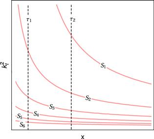 New window|Download| PPT slide
 New window|Download| PPT slide
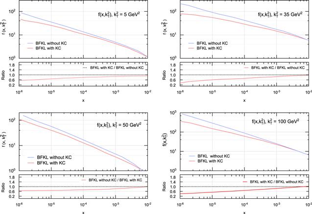 New window|Download| PPT slide
 New window|Download| PPT slide
 New window|Download| PPT slide
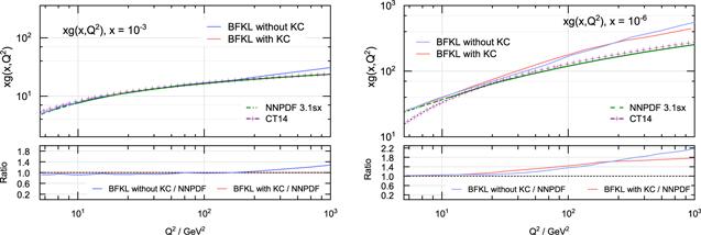 New window|Download| PPT slide
 New window|Download| PPT slide
 New window|Download| PPT slide
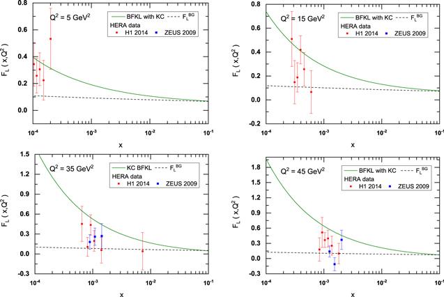 New window|Download| PPT slide