Quantum information and microscopic measuring instruments

删除或更新信息，请邮件至freekaoyan#163.com(#换成@)

本站小编 Free考研考试/2022-01-02

Alexey V Melkikh^,Ural Federal University, Yekaterinburg, Russia

Received:2019-08-20Revised:2019-10-22Accepted:2019-10-31Online:2019-12-27

Abstract
The consideration of measuring instruments as macroscopic bodies leads to neglect of the microscopic processes that occur during measurements. This disregard is not justified in general cases. As an example of measurements using microscopic instruments, the scattering of a photon by an electron with electron interference at two slits (Compton effect) was used. The amount of information that can be obtained in such a process is inversely proportional to the wavelength of the incident photon. At large photon wavelengths (soft measurements), the pure state of the electron can be disrupted by an arbitrarily small extent; accordingly, the amount of information extracted in such an experiment is also arbitrarily small. It is shown that the energy price for a bit obtained in such a measurement tends toward a constant value for increasing the photon wavelength. Microscopic instruments can be used in situations where energy costs for measurements are important.
Keywords： measurement problem;double-slit experiment;Von Neumann entropy;decoherence;compton effect

PDF (625KB)Metadata Metrics Related articlesExportEndNote|Ris|Bibtex Favorite
Cite this article
Alexey V Melkikh. Quantum information and microscopic measuring instruments. Communications in Theoretical Physics, 2020, 72(1): 015101- doi:10.1088/1572-9494/ab5453

1. Introduction

Despite the intensive development of theoretical and experimental studies of quantum information, a number of fundamental issues remain unresolved. Quantum information can ultimately be obtained only in measurements; moreover, the acquisition of such information is the purpose of measurements. In most cases, it is considered that measurements are carried out by classic instruments. For example, in experiments on quantum teleportation, it is assumed that both sides use classic instruments that measure the state of a quantum system over a certain basis (see, for example, [1–3]). However, in general cases, the instrument for information extraction may not be classic but can have microscopic dimensions and possess quantum properties. Microscopic instruments can be relevant both in terms of minimum energy consumption for measurement and in the sense of minimum spatial size. This phenomenon means that a microscopic measurement model is needed, including consideration of not only the limiting case of a classic instrument but also possible intermediate states, up to the case when only one particle is emitted (absorbed).

2. Quantum information and Von Neumann entropy

The qubit state is usually characterized by von Neumann entropy:(1)

$ \begin{eqnarray}S\left(\rho \right)=-{\rm{T}}{\rm{r}}\left(\rho \,\mathrm{ln}\,\rho \right).\end{eqnarray}$

This quantity is equal to zero for the pure state and coincides with the Shannon entropy in the case of a mixed state. It must, however, be noted that this formula was proposed by von Neumann as a generalization of Shannon’s formula for quantum processes. The Shannon formula, in turn, was proposed as analogous with the formula for physical entropy

$ \begin{eqnarray*}S=-\displaystyle \sum _{i}{p}_{i}\,\mathrm{ln}\,{p}_{i}.\end{eqnarray*}$

Indeed, there are a large number of variants of formulae for quantum entropy [4–6].

Since information is a broad concept that is not directly related to any particular type of physical carrier, such a value can be introduced for particles of any nature. For both electrons and photons, a density matrix can be introduced. This density matrix can characterize the system as a whole, including a measuring instrument.

How can information be obtained, for example, in the Stern–Gerlach experiment? In a number of works (see, for example, [7]), it is asserted that the very presence of a magnetic field makes this system an instrument via which information can be obtained. However, the magnetic field alone cannot lead to a violation of the coherence of the particle state. However, if the evolution of the particle remains unitary, then its von Neumann entropy remains equal to zero, and no additional information for the position of the particle can be extracted. To do this, we need to carry out the actual measurement. As will be shown below, for the process to be a measurement, the emission (absorption) of particles is necessary.

Thus, in the case of unitary evolution (in the absence of emission and absorption of particles), the von Neumann entropy cannot change, and, therefore, information cannot be obtained by any instrument. Obtaining information is possible only in the case of non-unitary evolution. This possibility is what characterizes the instrument as the recipient of information.

3. Microscopic measurement instrument and soft measurements

Since the purpose of measurements is simply to obtain information, then, to understand the mechanisms of information transfer, it is necessary to have a measurement model. A number of such models have been proposed earlier (see for example, [8–10]); however, in most works, the measurement instrument is considered macroscopic. In this case, the microscopic processes occurring during the measurement are neglected. This disregard is not justified in the general case.

In the paper [11], it was noted that the problem of measurements in quantum mechanics is closely related to the linearity of the Schrödinger equation. However, the Schrödinger equation is only an approximation of a more general system of equations for quantum particles and fields that is nonlinear. It is this nonlinearity that makes it possible to solve the measurement problem in quantum mechanics since, in general, the superposition principle for wave functions does not hold. In the work [11], it is assumed that the elementary process with which a measurement can be associated is the creation (annihilation) of particles.

The creation and annihilation of particles is described on the basis of the theory of inelastic scattering [12], the feature of which is the violation of coherence. The scattering process itself is described on the basis of the scattering matrix, which relates the states of the system before and after scattering. We emphasize (see also [13]) that the linear Schrödinger equation works only before and after scattering, but does not describe the process itself. The reason for this lack of description is that, first when the number of particles changes, their evolution cannot be described on the basis of a single equation since an ambiguity arises for the mass of the particle that should appear in it. Thus, the process of inelastic scattering is nonlinear.

At present, detectors are able to detect the state of individual microparticles. With the large variety of particle detectors, the elementary processes underlying their operation are few. The most common detectors are based on the photoelectric effect and the ionization of atoms. A characteristic feature of both processes is that the particles in them are emitted or absorbed. Without radiation or absorption of particles, there are no such processes that could become the basis of measurement.

One can imagine two limiting cases of instruments: when the energy for measurements is taken from the particle itself and when it is taken from the instrument. Between these limiting states, of course, there are an infinite number of intermediate variants. If we consider such a violation of unitarity as a process of decoherence, then it can be seen that the two limiting cases correspond to the terms ‘decoherence’ and ‘dephasing’ (see, for example, [8]).

We note the important property of a microscopic instrument: it is impossible to unambiguously divide the measured system and the instrument itself in the sense that, in another experiment, the instrument can be regarded as a measurable system, and vice versa. Thus, any of these signals, in principle, can be amplified to a macroscopic level and can be used to control the performance of work.

Further amplification of the signal for one particle can occur either by successively producing an increasing number of particles or by the production of a multitude of particles at once. We note, at the same time, that there is no reason to assert that the signal from one particle must necessarily be amplified to a macroscopic level. Most of our instruments are truly macroscopic, but this does not mean that the existence of microscopic instruments is prohibited. To clarify this question, it is necessary to define the term ‘instrument’ more accurately.

We can understand by the term ‘instrument’ such a system, the state of which to some extent corresponds to the state of the environment. Thus, there is a certain correlation between the state of the instrument and the measured parameter—a part of the environment (for example, particles). This definition is quite general and does not imply the macroscopic nature of the instrument. In the limit, the instrument can be one particle, the state of which changes as a result of interaction with the surrounding medium.

Taking into account the above, consider the simplest instrument that can be represented in the form of a two-level system—a qubit, located in the upper, long-lived state. When the qubit interacts with the particle being measured, the minimum possible exchange of energy occurs; the particle induces a qubit transition from the excited level to the ground level, accompanied by the emission of a photon. In the opposite case, the particle itself (photon) is absorbed by the qubit, which was initially in the ground state. A macroscopic instrument in this case can consist of a macroscopic number of coupled qubits.

A qubit can serve as an instrument for a photon, but a photon can also serve as an instrument for measuring the state of a qubit. In either case, the scattering process is nonlinear.

As it was shown earlier [11], the term ‘measurements without interaction’ is incorrect because, in any case, the creation (annihilation) of particles is necessary, which is impossible without interaction. In this regard, it is logical, however, to determine the measurement associated with the minimum impact on the system. Obviously, such a minimum effect must be accompanied by the emission of a particle with low energy (large wavelength). However, the accuracy of such a measurement will be small. We can call such a measurement soft.

An example of such a soft measurement can be an experiment using two slits. The purpose of such an instrument (which might not be macroscopic) is to determine which slit the electron passed through, wherein a flash on the screen is the result of the work of a macroscopic instrument—one of the many types of detectors. If, during the movement of the electron to the screen, we have the opportunity to act on it, for example, by scattering the particle, then we have the opportunity to determine through which slit the electron passed (see, for example, [14]). This case requires more detailed modeling and will be considered below.

Thus, as a result of the large number of particles created in the instrument, it, together with the particle being measured, passes into one of its states. Such a transition is accompanied by decoherence of the wave function of the particle being measured. It must be emphasized, however, that decoherence is the addition of a finite number of waves that can have a random phase. Only in the limit of an infinitely large number of such waves (a classical instrument) can we speak about a collapse of the wave function, i.e. that the particle is in a certain state. Theoretically, this property is expressed by the fact that the projection operator used in the theory of measurements is the cumulative effect of a large number of particle scattering events in the instrument. In general, the number of particles in the instrument is limited (or small), which will lead to partial decoherence. In this case, one cannot speak about the collapse of the wave function; nevertheless, the measurement takes place. Another question that remains is how much information can be obtained.

4. Entropy change in the measurement process with microscopic instrument

To answer the question about the amount of information that can be obtained in the measurement, let us use the classic results of the theory of quantum measurements. The density matrix of the pure state obeys the Liouville–von Neumann equation [15]:

$ \begin{eqnarray*}\displaystyle \frac{{\rm{d}}}{{\rm{d}}t}\rho \left(t\right)=-{\rm{i}}\left[H\left(t\right),\rho \left(t\right)\right]=L\left(t\right)\rho \left(t\right).\end{eqnarray*}$

According to [15], a change in entropy as a result of a nonselective quantum measurement can be defined as:

$ \begin{eqnarray*}{\rm{\Delta }}S=S\left(\rho ^{\prime} \right)-S\left(\rho \right).\end{eqnarray*}$

For an ideal measurement, we get:

$ \begin{eqnarray*}0\leqslant S\left(\rho \parallel \rho ^{\prime} \right)=-S\left(\rho \right)-{\rm{T}}{\rm{r}}\left\{\rho \,\mathrm{ln}\,\rho ^{\prime} \right\}.\end{eqnarray*}$

It can be shown [15] that

$ \begin{eqnarray*}S\left(\rho \parallel \rho ^{\prime} \right)=-S\left(\rho \right)+S\left(\rho ^{\prime} \right)\geqslant 0.\end{eqnarray*}$

This means that, for an ideal measurement, the von Neumann entropy cannot decrease. In the general case of generalized measurements, this is not true. If the density matrix does not change, then the change in entropy is zero in this measurement. Obviously, as a result of inelastic scattering, the density matrix always changes, which entails an increase in entropy.

If ρ₀ is the density matrix of the stationary state, that is

$ \begin{eqnarray*}V\left(t\right){\rho }_{0}={\rho }_{0},\end{eqnarray*}$

then the dynamic transformation reduces the relative entropy:

$ \begin{eqnarray*}S\left(V\left(t\right),\rho \parallel {\rho }_{0}\right)\leqslant S\left(\rho \parallel {\rho }_{0}\right).\end{eqnarray*}$

If we take

$ \begin{eqnarray*}V\left(t\right)=\exp \left(Lt\right),\end{eqnarray*}$

where L—is the Lindblad operator, according to [15] for the entropy production, we get:

$ \begin{eqnarray*}\sigma \left(\rho \left(t\right)\right)=-\displaystyle \frac{{\rm{d}}}{{\rm{d}}t}S\left(\rho \left(t\right)\parallel {\rho }_{0}\right)\geqslant 0.\end{eqnarray*}$

One of the simplest systems in the theory of decoherence is the two-level system (qubit) (e.g. [16]), where the environment is the modes of the boson field. The Hamiltonian in this model has the form:

$ \begin{eqnarray*}{H}_{{\rm{t}}{\rm{o}}{\rm{t}}}=\displaystyle \frac{\hslash \omega }{2}{\sigma }_{z}+\displaystyle \sum _{k}\hslash {\omega }_{k}{b}_{k}^{+}{b}_{k}+{\sigma }_{z}\displaystyle \sum _{k}\left({g}_{k}{b}_{k}^{+}+{g}_{k}^{* }{b}_{k}\right),\end{eqnarray*}$

where Σ_z is the Pauli spin operator, and g_k are the coupling constants.

Let us consider the interference of an electron with two slits. Our task is to determine which slit the particle passed through. This can be done, for example, by scattering a photon on a flying electron (Compton effect). Suppose that in such a scattering process the energy of the electron varies little, which corresponds to a large wavelength of the scattered photon. We will show that in this case the entropy production (equal to the speed of information creation in the measurement) is also small.

A small addition to the interaction Hamiltonian means that measurements on some basis almost did not occur. The instrument is not classic, and the received information is infinitely small. Therefore, it is logical to introduce the term ‘soft measurement’ for such a situation, which means that, as a result of such a measurement, an infinitesimal (or simply small in comparison with something) amount of information is obtained.

Then, the master Markov equation (quantum optical master equation in the Lindblad form (see, for example, [15]) can be obtained for the density matrix:(2)

$ \begin{eqnarray}\displaystyle \frac{{\rm{d}}}{{\rm{d}}t}{\rho }_{S}=-\displaystyle \frac{i}{\hslash }\left[{H}_{LS},{\rho }_{S}\right]+D\left[{\rho }_{S}\left(t\right)\right].\end{eqnarray}$

The second term on the right side is a dissipator. The structure of D is such that this function is proportional to the particle creation and annihilation operators. In the absence of the creation and annihilation of particles, D is zero, and the evolution of a quantum system becomes unitary and can be described by the Liouville–von Neumann equation.

For example, in the decay of a two-level system, the dissipator is proportional to the rate of spontaneous emission. This means that such a process, accompanied by the birth of a photon, is irreversible.

If the dissipator contains interaction with only one long-wavelength photon (that is, a particle passing through the slits is entangled with it and not with an entire set of bosons), then the term corresponding to such an interaction will be small in comparison with the basic Hamiltonian. This means that the contribution to the information obtained through this process is small compared with that of the main expression. In this case, the instrument for obtaining information does not have to be macroscopic. In this case, the interference pattern on the screen, which corresponds to the pure state of the system, only slightly ‘spoils.’

Thus, the notion of measurement as a projection onto a selected state is only the limiting case of a set of scattering events.

Consider the Lindblad equation of the form:

$ \begin{eqnarray*}\displaystyle \frac{{\rm{d}}}{{\rm{d}}t}\rho =-\displaystyle \frac{{\rm{i}}}{\hslash }\left[H,\rho \right]-\displaystyle \frac{\rho }{\tau }.\end{eqnarray*}$

Then, the entropy change for this case will have the form:

$ \begin{eqnarray*}\begin{array}{lll}\displaystyle \frac{{\rm{d}}}{{\rm{d}}t}S\left(\rho \right) & = & -{\rm{T}}{\rm{r}}\left(\left(-\displaystyle \frac{{\rm{i}}}{\hslash }\left[H,\rho \right]-\displaystyle \frac{\rho }{\tau }\right)\mathrm{ln}\,\rho \right)\\ & & -\,{\rm{T}}{\rm{r}}\left[-\displaystyle \frac{{\rm{i}}}{\hslash }\left[H,\rho \right]-\displaystyle \frac{\rho }{\tau }\right].\end{array}\end{eqnarray*}$

Here, τ is the characteristic decoherence time. Obviously, if this time is much larger than the time between measurements using a single particle, then the decoherence is small, and the information obtained in such a process is also small. When measuring using one photon, this time is of the order of:

$ \begin{eqnarray*}\tau \sim \displaystyle \frac{2\pi }{\omega },\end{eqnarray*}$

where ω—is the frequency of the emitted photon. Thus, soft measurements (in which long-wavelength photons are emitted) cannot be performed quickly.

Measurement involves the participation of real particles. In this case, the creation (absorption) of one particle is an elementary act of measurement.

5. Control of qubits and the measurement of their states

The qubit is one of the simplest quantum systems; thus, the consideration of the measurement problem for such a system is the most obvious. However, measuring the state of qubits is one of the most important operations in the operation of a quantum computer (see, for example, [17, 18]).

Consider, for example, as a qubit, the spin in a magnetic field with two possible states. The control of such a qubit is carried out using a polarized alternating magnetic field. As a result, Rabi oscillations arise. At the same time, the population is completely pumped from one level to another in a time:

$ \begin{eqnarray*}\tau =\displaystyle \frac{\pi }{2{\rm{\Omega }}},\end{eqnarray*}$

where ω—is the frequency of the changing magnetic field.

Such a control is unitary since the particles are not created and do not disappear, and the magnetic field is classic. In this case, the qubit dynamics are described by the linear Schrodinger equation. The effect of a magnetic field is fundamentally different from the scattering of photons in that in the first case, the creation or annihilation of particles does not occur, and this process is linear. The scattering process is essentially nonlinear. The same conclusion can be attributed to the Stern–Gerlach experiment: the magnet itself cannot be recognized as an instrument since the dynamics of particles in it are unitary; in this case, the instrument is the sensor with which particles are recorded.

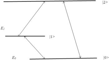
How is the qubit measured on the basis of 01?A state of the qubit is ‘queried’ by a laser with a certain wavelength. If the qubit was in state 0, it will go to state 2. After the spontaneous return of the qubit to state 0, a photon will be emitted, which gives the required information. If the qubit was in state 1, there will be no photon emission. To prevent the ion from remaining at a metastable level, another laser is turned on. Spontaneously emitted photons are measured with a detector. It takes time to accumulate a significant signal. There are also other methods for measuring the state of qubits. The scheme of the qubit levels is shown in figure 1 [19].

Figure 1.

New window|Download| PPT slide
Figure 1.The scheme of the qubit levels.

This is the main difference in the control of qubits with the help of unitary operations (for example, a magnetic field) from the measurement of the state of the qubits. The latter process is necessarily accompanied by the creation (annihilation) of particles and cannot be described on the basis of the Schrödinger equation.

We also note that the spontaneous transition of a qubit from the upper to the lower level can be described only in the framework of quantum field theory. The characteristic time of existence for the qubit at the upper level is connected with the finiteness of the width of the energy level due to the interaction of an electron with virtual particles.

Since the width of the qubit energy levels is always finite, there is a small probability that it will absorb a photon with a wavelength much greater than that corresponding to the difference in its level. It is in this case that the concept of ‘soft measurement’, introduced above, makes sense. In other words, this is a measurement in which the interference pattern is broken slightly. In this case, the qubit state will be measured with a small accuracy, which depends on the wavelength of the photon. As noted above, the softer the measurement is, the less information about the state of the qubit of such a measurement can be obtained.

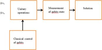
Operations with qubits form the basis of a quantum computer, the schematic diagram for which is shown in figure 2.

Figure 2.

New window|Download| PPT slide
Figure 2.Schematic diagram of quantum computer.

It should be noted that, generally speaking, it is impossible to divide the operations of unitary control and measurement for arbitrary measurements. This means that the output of the quantum computer will have a ‘softly’ measured state for the register. This state will represent the solution of the problem in the most general form.

6. The model of electron interference at two slits for intermediate irradiation by a photon: Compton effect

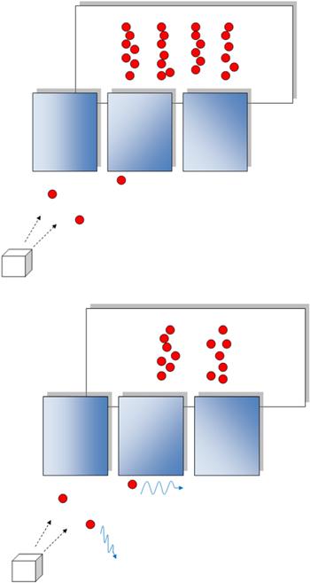
The Compton effect is the scattering of a photon by an electron. This effect finds a variety of technological applications (see, for example, [19]). Consider the Compton effect when measuring the passage of an electron through two slits and find how much information can be obtained as a result of such a process. If the experiment is repeated many times, then we can introduce the von Neumann entropy for the initial and final states of the electron, as well as for the photon with which the measurement takes place.

Let us consider the interference of electrons at two slits, taking into account that an electron can interact with a photon along the way (figure 3).

Figure 3.

New window|Download| PPT slide
Figure 3.Smearing of the interference pattern for the intermediate scattering of photons by an electron.

Let the electron and photon before the collision move along the x-axis; then, we can write the equations for the conservation of energy and momentum for the system:

$ \begin{eqnarray*}\displaystyle \frac{hc}{\lambda }+c\sqrt{{p}_{0}^{2}+{m}_{0}^{2}{c}^{2}}=\displaystyle \frac{hc}{\lambda ^{\prime} }+c\sqrt{{p}^{2}+{m}_{0}^{2}{c}^{2}},\end{eqnarray*}$

$ \begin{eqnarray*}\displaystyle \frac{h}{\lambda }+{p}_{0}=\displaystyle \frac{h}{\lambda ^{\prime} }\,\cos \,{\rm{\Theta }}+{p}_{x},\end{eqnarray*}$

$ \begin{eqnarray*}0=\displaystyle \frac{h}{\lambda ^{\prime} }\,\sin \,{\rm{\Theta }}+{p}_{y}.\end{eqnarray*}$

Figure 4.

New window|Download| PPT slide
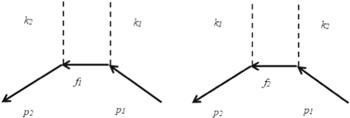
Figure 4.Feynman diagrams for Compton effect.

Figure 5.

New window|Download| PPT slide
Figure 5.Optical paths for electron interference at two slits.

Solving this system of equations, we can determine how the de Broglie wavelength of an electron changes as a result of the scattering of a photon. We obtain for the electron momentum:

$ \begin{eqnarray*}p={p}_{0}\sqrt{{\left(\alpha +\sqrt{1+\beta }-\displaystyle \frac{\alpha \sqrt{1+\beta }}{\left(\alpha +\sqrt{1+\beta }-\cos {\rm{\Theta }}\left(\alpha +1\right)\right)}\right)}^{2}-\beta },\end{eqnarray*}$

where

$ \begin{eqnarray*}\alpha =\displaystyle \frac{h}{\lambda {p}_{0}},\beta =\displaystyle \frac{{m}_{0}^{2}{c}^{2}}{{p}_{0}^{2}}.\end{eqnarray*}$

We note that the simplified theory for the Compton effect does not enable us to determine all the scattering characteristics (in particular, the angle). The exact relativistic theory for the Compton effect was formulated within the framework of QED. In the second order of perturbation theory, Compton scattering is described by two Feynman diagrams [20, 21]. The matrix element contains four-dimensional momenta for the virtual electrons (f₁ and f₂) for which the usual relationship between momentum and energy is not satisfied.

$ \begin{eqnarray*}\begin{array}{lll}\langle f| {S}^{(2)}| i\rangle & = & \displaystyle \frac{{\rm{i}}{e}^{2}}{4\sqrt{{\omega }_{1}{\omega }_{2}{\varepsilon }_{1}{\varepsilon }_{2}}}{(2\pi )}^{4}\delta ({p}_{1}+{k}_{1}-{p}_{2}-{k}_{2})\\ & & \times \,{\bar{u}}_{2}\left\{{\hat{e}}_{2}* \displaystyle \frac{{\rm{i}}{\hat{f}}_{1}-m}{{f}_{1}^{2}+{m}^{2}}{\hat{e}}_{1}+{\hat{e}}_{1}\displaystyle \frac{{\rm{i}}{\hat{f}}_{2}-m}{{f}_{2}^{2}+{m}^{2}}{\hat{e}}_{2}* \right\}{u}_{1}.\end{array}\end{eqnarray*}$

Two Feynman diagrams correspond to the two terms in the matrix element (figure 4) [20]:

As a result, the Klein–Nishina formula for the differential scattering cross section [20] was obtained

$ \begin{eqnarray*}{\rm{d}}\sigma =\displaystyle \frac{1}{{r}_{0}^{2}}{\left(\displaystyle \frac{{\omega }_{2}}{{\omega }_{1}}\right)}^{2}\left(\displaystyle \frac{{\omega }_{2}}{{\omega }_{1}}+\displaystyle \frac{{\omega }_{1}}{{\omega }_{2}}-{\sin }^{2}\theta \right){\rm{d}}{o}_{2}.\end{eqnarray*}$

At low photon energies, the formula for the differential cross section for the scattering of photons with respect to the angles goes over into the well-known Thompson formula.

The wavelength of an electron before a collision is

$ \begin{eqnarray*}{\lambda }_{e}=\displaystyle \frac{h}{{p}_{0}}.\end{eqnarray*}$

Then, after a collision, the wavelength will be:

$ \begin{eqnarray*}{\lambda }_{e}^{\prime} =\displaystyle \frac{{\lambda }_{e}}{\sqrt{{\left(\alpha +\sqrt{1+\beta }-\displaystyle \frac{\alpha \sqrt{1+\beta }}{\left(\alpha +\sqrt{1+\beta }-\cos {\rm{\Theta }}\left(\alpha +1\right)\right)}\right)}^{2}-\beta }}.\end{eqnarray*}$

According to the classic results of wave optics, following the addition of two coherent waves, their phase difference will be:

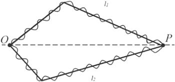
$ \begin{eqnarray*}\delta =\displaystyle \frac{2\pi }{{\lambda }_{0}}{\rm{\Delta }}=\displaystyle \frac{2\pi }{{\lambda }_{0}}\left({n}_{2}{l}_{2}-{n}_{1}{l}_{1}\right),\end{eqnarray*}$

where Δ—is the optical path difference, n₁, n₂ are the refractive indices for the two waves, and l₁, l₂ are their geometric paths. In accordance with this, the change in the contribution to the phase for an electron in the case when scattering occurs on one path will be:

$ \begin{eqnarray*}\begin{array}{l}\displaystyle \frac{2\pi {l}_{2}}{{\lambda }_{e}^{\prime} }-\displaystyle \frac{2\pi {l}_{2}}{{\lambda }_{e}}\,=\,2\pi {l}_{2}\displaystyle \frac{{p}_{0}}{h}\left(\sqrt{{\left(\alpha +\sqrt{1+\beta }-\displaystyle \frac{\alpha \sqrt{1+\beta }}{(\alpha +\sqrt{1+\beta }-\cos {\rm{\Theta }}(\alpha +1))}\right)}^{2}-\beta }-1\right).\end{array}\end{eqnarray*}$

Here, l₁ and l₂ are the optical paths for the interference pattern (figure 5).

For an estimate, we can specify a certain average scattering angle. It is easy to see that at large wavelengths for the incident photon, the contribution to the phase will be arbitrarily small. In this case, the scattering angle will not play a significant role. This means that the interference pattern will almost not be ‘spoiled’ by a photon.

If the photon momentum is much smaller than the electron momentum,

$\alpha =\tfrac{h}{\lambda {p}_{0}}\ll 1,$

and the velocity of electron is much less than the speed of light,

$\beta =\tfrac{{m}_{0}^{2}{c}^{2}}{{p}_{0}^{2}}\gg 1,$

we get:

$ \begin{eqnarray*}\delta =-\displaystyle \frac{2\pi {l}_{2}}{\lambda }\,\cos \,{\rm{\Theta }}.\end{eqnarray*}$

The contribution to the phase can be either positive or negative depending on the angle of scattering of the photon. For example, when a photon is scattered backward relative to the initial direction of motion, the cosine will be negative, and therefore the contribution to the phase will be positive (the wavelength of the electron after the collision will be less than the wavelength before the collision). Consideration of scattering along other axes leads to similar formulas.

Thus, if the wavelength of the photon becomes of the order of the path that the electron takes to travel to the screen, the interference pattern on the screen disappears. However, in fact, it will disappear earlier because when the wavelength of the photon becomes comparable with the distance between the slits d, we can no longer guarantee that the photon will interact with the electron on its left (right) path. At the same time, with interference, the following relation always holds:

$ \begin{eqnarray*}d\ll l,\end{eqnarray*}$

where l denotes any of the paths.

For an infinitesimal disturbance of the interference pattern, the information (equal to the change in entropy) obtained in such a process will also be infinitely small:

$ \begin{eqnarray*}{\rm{\Delta }}S\sim \displaystyle \frac{1}{\lambda }.\end{eqnarray*}$

Indeed, consider the production of von Neumann entropy:

$ \begin{eqnarray*}\displaystyle \frac{{\rm{d}}}{{\rm{d}}t}S\left(\rho \right)=-{\rm{T}}{\rm{r}}\left(\displaystyle \frac{{\rm{d}}\rho }{{\rm{d}}t}\,\mathrm{ln}\,\rho \right)-{\rm{T}}{\rm{r}}\left(\displaystyle \frac{{\rm{d}}\rho }{{\rm{d}}t}\right).\end{eqnarray*}$

The second term from the normalization condition is zero. Thus, we have:

$ \begin{eqnarray*}\displaystyle \frac{{\rm{d}}}{{\rm{d}}t}S\left(\rho \right)=-{\rm{T}}{\rm{r}}\left(\displaystyle \frac{{\rm{d}}\rho }{{\rm{d}}t}\,\mathrm{ln}\,\rho \right).\end{eqnarray*}$

Taking into account equation (2), we obtain:

$ \begin{eqnarray*}\displaystyle \frac{{\rm{d}}}{{\rm{d}}t}S\left(\rho \right)=-{\rm{T}}{\rm{r}}\left(\left[-\displaystyle \frac{{\rm{i}}}{\hslash }\left[{H}_{LS},{\rho }_{S}\right]+D\left[{\rho }_{S}\left(t\right)\right]\right]\mathrm{ln}\,\rho \right).\end{eqnarray*}$

The first term is zero since this is the entropy production corresponding to unitary evolution, which is zero. Thus, we get:

$ \begin{eqnarray*}\displaystyle \frac{{\rm{d}}}{{\rm{d}}t}S\left(\rho \right)=-{\rm{T}}{\rm{r}}\left(D\left[{\rho }_{S}\left(t\right)\right]\mathrm{ln}\,\rho \right).\end{eqnarray*}$

We introduce the frequency with which the photons fall on the electrons passing to the screen. In fact, such a frequency ν will be the frequency with which measurements are made. Then, the entropy production will be proportional to the following ratio:

$ \begin{eqnarray*}\displaystyle \frac{{\rm{d}}}{{\rm{d}}t}S\left(\rho \right)\sim \nu \displaystyle \frac{\omega }{{\omega }_{0}}.\end{eqnarray*}$

Here, ω is the frequency of the photon-instrument, and ω₀ is the de Broglie frequency of the electron. Therefore, in one measurement act, information for the order of the frequency ratio can be obtained:

$ \begin{eqnarray*}I={\rm{\Delta }}S\sim \displaystyle \frac{\omega }{{\omega }_{0}}.\end{eqnarray*}$

At low frequencies (large photon-instrument wavelengths), this information will be arbitrarily small. This is the case for soft measurements. If the quality of the instrument was exhausted by the amount of information received, then soft measurements would always be ineffective. However, the energy costs for obtaining such information can also be important. With a lack of energy, this factor can turn out to be a limiting factor.

In particular, what will be the price of the received bit of information?If the information is divided into the energy of the emitted photon (particle)

$\hslash \omega ,$

then it can be found that the energy price for one bit of information obtained with a soft measurement tends to some constant value independent of the properties of the photon.

One can also ask the following question: in what sense can a photon interacting with an electron be regarded as a measuring instrument?Obviously, the result of the measurement should be information about the slit through which the electron passed. Thus, if we consider a photon as a measuring instrument, the disappearance of the interference pattern signal is meaningful only if we can guarantee that the photon has interacted with an electron that has passed through a certain slit.

Thus, the destruction of the interference pattern for the case of the Compton effect is naturally explained using a scattering mechanism that does not require additional assumptions about the macroscopic nature of the instrument and the collapse of the wave function. We emphasize that the calculation for the interaction of an electron and a photon (and hence the calculation for the measurement process as such) is possible only within the framework of quantum field theory. This, on the other hand, means that the calculation of the amount of information obtained in this way is also possible only within the framework of quantum field theory.

The interaction of an electron and a photon is one of the simplest processes of inelastic scattering. Arbitrary inelastic scattering processes are solved exactly only in the framework of QED. This means that the very problem of measurements in quantum mechanics can be solved only within the framework of QED.

What is the relationship between microscopic and macroscopic instrument?A macroscopic instrument can often be considered as a large number of microscopic instruments connected to each other in a certain way. As a result of such a connection, the signal of the microscopic instrument is amplified to a macroscopic level. The combination (parallel or serial connection) of such microsystems is a classic instrument. Since, as a result of the passage of a measured particle through all microscopic instruments, its phase receives independent additives each time, in the end, the particle trajectory can be determined, since quantum interference is completely destroyed by these additives.

As one of the simplest examples, consider the classic Geiger counter. When a detected particle enters a volume with a gas, it can ionize one of its atoms; in this case, an ion and electron appear, with the particle itself losing its energy. The ion and electron are accelerated in the electric field, which causes ionization of the following particles, etc. We emphasize that, in principle, the particle is measured after ionization of the first atom. Already, such a microscopic signal, in principle, can be used as a control in any process.

A photoelectric effect is often used for registration of photons. When a photon falls on the surface of a photovoltaic cell, an electron is knocked out of it, which, getting into the photoelectron multiplier, leads to the appearance of an increasing avalanche of electrons. Ultimately, the signal becomes macroscopic.

Other examples include particle detectors such as scintillators and an ionization calorimeter.

All these instruments are macroscopic, but in some cases (measurements inside a living cell, nanotechnology), it may be necessary to use microscopic instruments.

7. Conclusion

The requirement of a macroscopic nature for a measuring instrument leads to neglect of the microscopic processes that occur during the measurement. This disregard is not justified in general cases. As an example of a microscopic instrument, the scattering of a photon by an electron with electron interference at two slits (the Compton effect) is considered. The amount of information that can be obtained in such a process, which turns out to be inversely proportional to the wavelength of the incident photon, is calculated. At large photon wavelengths, the pure state of an electron can be disrupted by an arbitrarily small extent; accordingly, the amount of information extracted in such an experiment is just as arbitrarily small. However, the energy price of the bit of information obtained in such a measurement with a rise in the wavelength tends toward a constant value for increasing of the wavelength of the photon. Microscopic instruments can be relevant in situations where the energy costs of measurements are limiting factors.

Reference By original order
By published year
By cited within times
By Impact factor

[1]

Bennett

C H

Brassard

Crepeau

Jozsa

Peres

Wootters

W K

1993 Phys. Rev. Lett. 70 1895

DOI:10.1103/PhysRevLett.70.1895 [Cited within: 1]

[2]

Peres

Terno

D R

2004 Quantum information and relativity theory
Rev. Mod. Phys. 76 93

DOI:10.1103/RevModPhys.76.93

[3]

Horodecki

2009 Rev. Mod. Phys. 81 865

DOI:10.1103/RevModPhys.81.865 [Cited within: 1]

[4]

Accardi

Ohya

Watanabe

1996 Rep. Math. Phys. 38 457

DOI:10.1016/S0034-4877(97)84895-1 [Cited within: 1]

[5]

Watanabe

2016 Phil. Trans. R. Soc. A 374 20150240

DOI:10.1098/rsta.2015.0240

[6]

Watanabe

2015 Found. Phys. 45 1311

DOI:10.1007/s10701-015-9925-2 [Cited within: 1]

[7]

Peacock

K A

Hepburn

P S

1999(arXiv:quant-ph/9906036)

[Cited within: 1]

[8]

Schlosshauer

2004 Rev. Mod. Phys. 76 1267

DOI:10.1103/RevModPhys.76.1267 [Cited within: 2]

[9]

Allahverdyan

A E

Balian

Nieuwenhuizen

T M

2013 Phys. Rep. 525 1

DOI:10.1016/j.physrep.2012.11.001

[10]

Gurvitz

2016 Fortschr. Phys. 65 1600065

DOI:10.1002/prop.201600065 [Cited within: 1]

[11]

Melkikh

A V

2015 Commun. Theor. Phys. 64 47

DOI:10.1088/0253-6102/64/1/47 [Cited within: 3]

[12]

Landau

L D

Lifshitz

E M

1977 Quantum Mechanics: Non-Relativistic TheoryNew YorkPergamon

[Cited within: 1]

[13]

Melkikh

A V

2017 Mod. Phys. Lett. B 31 1750007

DOI:10.1142/S0217984917500075 [Cited within: 1]

[14]

Feynman

R P

Leighton

R B

Sands

1965 The Feynman Lectures on PhysicsReading, MAAddison-Wesley

[Cited within: 1]

[15]

Breuer

H P

Petruccione

2002 The Theory of Open Quantum SystemsOxfordOxford University Press

[Cited within: 5]

[16]

Hornberger

2009 Introduction to decoherence theory
Entanglement and Decoherence vol 768Lecture Notes in PhysicsBuchleitner

et al.BerlinSpringer221276

[Cited within: 1]

[17]

Nielsen

Chuang

2000 Quantum Computing and Quantum InformationCambridgeCambridge University Press

[Cited within: 1]

[18]

Valiev

K A

2005 Phys.-Usp. 48 1

DOI:10.1070/PU2005v048n01ABEH002024 [Cited within: 1]

[19]

Kaminska

et al.2016 Eur. Phys. J. C 76 445

DOI:10.1140/epjc/s10052-016-4294-3 [Cited within: 2]

[20]

Akhiezer

A I

Berestetskii

V B

1965 Quantum ElectrodynamicsNew YorkWiley

[Cited within: 3]

[21]

Berestetskii

V B

Lifshits

E M

Pitayevskii

L P

1982 Relativistic Quantum TheoryOxfordPergamon

[Cited within: 1]