Sino-French Institute of Nuclear Engineering and Technology, Sun Yat-sen University, Zhuhai 519082, China Received Date:2021-07-07 Available Online:2021-12-15 Abstract:Hundreds of thousands of experimental data sets of nuclear reactions have been systematically collected, and their number is still growing rapidly. The data and their correlations compose a complex system, which underpins nuclear science and technology. We model the nuclear reaction data as weighted evolving networks for the purpose of data verification and validation. The networks are employed to study the growing cross-section data of a neutron induced threshold reaction (n,2n) and photoneutron reaction. In the networks, the nodes are the historical data, and the weights of the links are the relative deviation between the data points. It is found that the networks exhibit small-world behavior, and their discovery processes are well described by the Heaps law. What makes the networks novel is the mapping relation between the network properties and the salient features of the database: the Heaps exponent corresponds to the exploration efficiency of the specific data set, the distribution of the edge-weights corresponds to the global uncertainty of the data set, and the mean node weight corresponds to the uncertainty of the individual data point. This new perspective to understand the database will be helpful for nuclear data analysis and compilation.
HTML
--> --> --> I.INTRODUCTIONNuclear reaction data underpin nuclear science and technology [1, 2]. One of the most important works in nuclear physics is to measure the nuclear reactions and reduce the data uncertainties in order to achieve the accuracy requirements in fundamental research fields, such as nuclear astrophysics [3, 4], and many application fields, such as transmutation of nuclear waste [5] and design of future nuclear reactors [6]. Since 1935, tens of thousands of experiments have been performed and hundreds of thousands of experimental data sets have been systematically collected to develop the experimental nuclear reaction databases, among which the most important and complete one is EXFOR [7]. In addition to this, evaluation and prediction using the historical data have also attracted attention, resulting in various international nuclear data libraries, such as ENDF [8], CENDL [9], JEFF [10], JENDL [11], and BROND [12]. Among the methods for data evaluation and prediction, nuclear reaction models combined with the generalized least squares method have gained prominence [13]. Successful applications of Monte Carlo evaluation methods based on the Bayesian statistical inference have also been reported [14, 15]. To solve illinversed regression problems for prediction with uncertainty quantification, machine learning, which is a very powerful tool to learn complex big data, has been applied [16, 17]. In the past decade, investigations on advanced reactor systems have defined new accuracy and scope requirements for nuclear reaction data [1]. To this end, huge investments have been devoted to salaries, equipment, and working hours for measuring new data. Meanwhile, statistical verification and validation is an effective means for quality improvement of the rapidly growing data [18]. The growth of the nuclear reaction data is actually an innovation process, which is intrinsic for the human experience. In this respect, fruitful research on complex networks [19-22] has made it possible to model and quantify the innovation. In fact, the abstract process of innovation has been investigated in different domains including linguistics [23], biology [24], economics [25], knowledge [26], and science [27]. Many empirical analyses of real-world discovery processes have demonstrated that the basic signature of the innovation process is the Heaps law [28-30], which was originally introduced to describe the number of distinct words in a text document [31]. Various models have proven that the Heaps law well describes the pace at which scientists discover concepts or users collect new items [32, 33]. In the case of science, different networks have been extracted from scholars, projects, papers, patents, ideas, and/or academic positions [27, 34]. Investigation of the key network properties offers a quantitative understanding of the interactions among scientific agents and quantitative insight into the evolution of individual scientific impact [35, 36]. This work is devoted to modeling the discovery process of the nuclear reaction data as a weighted evolving network. It is expected to map the salient features of the database to network properties so that the global uncertainty of the specific data set and the uncertainty of the individual data point can be quantified. The paper is organized as follows. In Sec. II, we describe the Bayesian Gaussian CANDECOMP/PARAFAC (BGCP) tensor decomposition model and the method to compose the networks. In Sec. III, we present both the results and discussion. Finally, a summary is given in Sec. IV.
II.METHODThe cross-section in a specific reaction channel, such as (n,2n) reaction, depends on the change and neutron numbers of the target and the incident energy. Let us discretize the energy degree of freedom using the energy gap $ {\rm d}E $; the data can then be represented by a three order missing tensor. Nowadays, tensor completion is widely used in image inpainting [37] and data imputation [38]. There are various types of non-Bayesian tensor completion techniques; for example, Liu et al. proposed an algorithm for missing values completion in visual data [39]. The beginning of the Bayesian model in the matrix completion area was introduced by Salakhutdinov and Mnih, who built the models of Bayesian matrix factorization [40]. Kolda and Bader gave a comprehensive review of tensor decomposition [41]. Xiong et al. combined the tensor decomposition with Bayesian inference considering the time dependency of each tensor [42]. Chen et al. recently proposed a Bayesian Gaussian CANDECOMP/PARAFAC (BGCP) tensor decomposition model without the time structure [43], which is taken into account in this work. We denote by $ {\cal{S}}\in{\mathbb{R}}^{I\times J\times K} $ the actual value of the tensor, where the entry $ \sigma_{ijk} $ is the physical reality of the cross section in the reaction of the target $ ^{2i+j}_{i}X_{i+j} $ at the incident energy $ E = k\cdot {\rm d}E $. Here, j denotes the isospin degrees of freedom, expressed as the difference between neutron and charge numbers $ j = N-Z $. Indeed, we do not have the values of $ \sigma_{ijk} $ but some observations with uncertainties. Considering the multiple measurements, let $ \sigma_{ijk}^{(p)} $ ($ p = 1,\cdots,P_{ijk} $) represent the p-th observation of the cross-section and $ P_{ijk} $ the total number of observations. A list of missing tensors $ {\widetilde{\cal{S}}} = \{ {\cal{S}}^{(1)},\ldots,{\cal{S}}^{(P)} \} $ could be used to describe all the observations, where $ P = \max(P_{ijk}) $ for all possible $ ijk $. The observations are arranged in the missing tensors according to their superscripts, such as $ \sigma_{ijk}^{(1)} $ in $ {\cal{S}}^{(1)} $, $ \sigma_{ijk}^{(2)} $ in $ {\cal{S}}^{(2)} $, and so on. The entries for no observations are missing. Being different from Ref. [43], the multiple observations for the physical reality $ \sigma_{ijk} $ are considered. In the following, we expound the resulting changes of the Bayesian framework of parameters. It is assumed that the uncertainty of each observed value follows an independent Gaussian distribution,
where $ \tau_{\epsilon} $ is the precision. In real-world applications the expectation $ \sigma_{ijk} $ is unknown and replaced with the estimated value $ \hat{\sigma}_{ijk} $, which is the entry of the estimated tensor $ {\hat{\cal{S}}} $. The CP decomposition is applied to calculate the estimation $ {\hat{\cal{S}}} $:
where $ {\boldsymbol{z}}_{l}\in{\mathbb{R}}^{I} $, $ {\boldsymbol{d}}_{l}\in{\mathbb{R}}^{J} $, and $ {\boldsymbol{e}}_{l}\in{\mathbb{R}}^{K} $ are respectively the l-th column vector of the factor matrices $ {\boldsymbol{Z}}\in{\mathbb{R}}^{I\times L} $, $ {\boldsymbol{D}}\in{\mathbb{R}}^{J\times L} $, and $ {\boldsymbol{E}}\in{\mathbb{R}}^{K\times L} $. The symbol $ \circ $ represents the outer product. The prior distribution of the row vectors of the factor matrix Z is the multivariate Gaussian
where the hyper-parameter $ {\boldsymbol{\mu}}^{(z)}\in{\mathbb{R}}^{L} $ expresses the expectation, and $ {\bf{\Lambda}}^{(z)}\in{\mathbb{R}}^{L\times L} $ indicates the width of the distribution. The likelihood function can be written as
where $ \circledast $ is the Hadamard product. The posterior values of the hyper-parameters $ {\boldsymbol{\mu}}^{(z)} $ and $ {\bf{\Lambda}}^{(z)} $ are given as
The contribution of the observations to the hyper-parameter is equivalent, being independent of which missing tensor it is arranged in. The likelihood function of all observations is
Based on Eq. (8), each observation contributes to the increase of $ \dfrac{1}{2} $ in $ \hat{a}_0 $, and $ \dfrac{1}{2}(x_{\bf{i}}^{(p)}-\hat{x}_{\bf{i}})^2 $ in $ \hat{b}_0 $. Equation (5) shows that the observations with the same subscript i contribute to the posterior values of the hyper-parameter $ {\boldsymbol{\mu}}_{i}^{(z)} $. Changing the second formula in Eq. (5) to
The weighted network can be built, where nodes are the observations, and the weight of the link between two observations with the same subscript is defined as
Cases for the subscripts j and k are similar. In Fig. 1, the above method is illustrated . In brief, as with the image inpainting, the cross-section in a specific reaction channel is represented by a three order tensor $ {\cal{S}} $. According to the CP decomposition, the tensor $ {\cal{S}} $ is expressed as the outer product of the factor matrixes Z, D, and E. The prior distributions of the factor matrixes are assumed to be multivariate Gaussians. With the observed data of the cross-section, the posterior values of the factor matrixes and their distributions can be calculated using Bayesian inference and iteration. Finally, the predicted cross-section is reconstituted with the factor matrixes Z, D, and E, while the network is built with the hyper-parameter μ and $ \Delta {\boldsymbol{\mu}} $. Figure1. (color?online)?Illustration for visualizing the definitions of the involved quantities and their relations.
III.RESULTS AND DISCUSSIONThe pioneers in measuring the (n,2n) reaction were Fowler and Slye, who measured the cross-sections in $ ^{63} {\rm{Cu}}$(n,2n)$ ^{64} {\rm{Cu}}$ reactions near the threshold [44]. After decades, measurement technology and deuterium-tritium (D-T) neutron generators became widely used, resulting in the linear growth of the data points (mainly around the incident energy 14 MeV). By 1980, a good deal of data measured between the threshold and 20 MeV using the pulsed neutron source at Bruyères-le-Chatel were published [45]. After that, owing to continuing investment in salaries, equipment, and working hours, the data points grew linearly. To date, 7671 cross-section data points of (n,2n) reaction (including 98 derived data) are recorded in the EXFOR database. Their annual growth is shown in Fig. 2(a). Figure2. (color online) Growth of nuclear reaction data and their evolving networks. Annual growth cross-section data of (a) (n,2n) reaction and (b) (γ,xn) reaction in the EXFOR database. Network generated from the (n,2n) cross-section data published before (c) 1960 and (d) 1965. The size and color of a node represent the degree $ k_{m} $ of a node m.
The discovery of the photoneutron reaction may date back to 1956, when the cross-section of a $ ^{6} {\rm{Li}}( \gamma ,{{x}}){{n}}$ reaction was measured by Edge [46]. Subsequently, the published data of this reaction grew rapidly. Due to the proven technology to provide a monoenergetic photon beam, the cross-section data for most of the stable nuclei have been measured within 20 years of its discovery. After 1980, only a few data were published because the scientific interest moved to more subdivided channels, such as (γ,n), (γ,2n) and so on. Twelve thousand data points have been collected in the EXFOR database. Their annual growth is shown in Fig. 2(b). Those two sets of nuclear reaction data are modeled respectively as the weighted evolving networks using the BGCP approach. The nodes in the networks are the data points and weights of the links are computed from the relative deviation between the data points. An example of the network is displayed in Fig. 2(c), where 362 data points published before 1960 are considered. The nodes, links, and numbers of neighbors are visualized clearly. The complexity of the network increases with increasing node number. Another example is shown in Fig. 2(d), where 1251 nodes are included, but the links are too numerous to recognize in the figure. The degree $ k_{m} $ of a node m is the number of edges linked with the node (the number of neighbors of node m). As shown in Fig. 3(a), the mean degrees and the node number in both networks grow approximately proportionally. It is an inevitable consequence of the discovery processes, where an experiment usually probes new data on the basis of verifying existing data. The slope reveals the innovativeness. A decrease in the slope indicates the emergence of new technologies for detecting new isotopes or a new incident energy region. A representative example is the slowdown of the mean degree $ \langle k_{m}\rangle $ in the (n,2n) network near $ N_{\rm node} $ = 4000, which results from the extension of the neutron beam from 14 MeV to the threshold. Figure3. (color?online)?Properties of the evolving small-world networks. (a) Mean degree of a node $ \langle k_{m}\rangle $, (b) mean weight of edges $ \langle w_{mn} \rangle $, (c) clustering coefficient C, (d) global efficiency E, and (e) number of novelties S of the graph as a function of node number.
In a weighted graph, the node strength $ s_{m} $ is defined as the summation of the edge-weights linked with a node. It integrates the information on the number and the weights of links. The mean strength in both networks also increases linearly with increasing node number. In contrast, a more interesting property is the mean weight of the edges in the graph, as shown in Fig. 3(b). It is found that not only the number (mean degree $ \langle k_{m}\rangle $) but also the weights (mean weight $ \langle w_{mn} \rangle $) of links increase during the growth of both networks. However, for the (n,2n) reaction, an approximate platform for the mean weight $ \langle w_{mn} \rangle $ appears for $ N_{\rm node} > $ 3000. The weight $ w_{mn} $ describes the linking strength between two nodes, while its reciprocal $ l_{mn} = 1/w_{mn} $ naturally expresses their relative distance in the network. Once $ \{ l_{mn} \} $ is given, it can be used to calculate the matrix of the shortest path length $ d_{mn} $ between two generic nodes i and j. The so-called clustering coefficient C and the global efficiency E of the graph can then be calculated [22]. The clustering coefficient C is also considered as the first approximation of the local efficiency. By using those efficiencies, both the local and global behaviors in small-world networks can be studied [19, 20]. The large C values and small E values in the early network indicate that the early data are locally clustered [see example in fig. 2(c)]. It is proven that the local verification and validation of the data are effective, where data of same isotope and similar incident energy are compared. This local method has been widely applied to date. With the growth of the networks, the clustering coefficients C decrease, while the global efficiencies E increase. The networks generated by the latest experimental data sets have C = 0.58 and E = 0.40 in the (n,2n) network, and C = 0.65 and E = 0.45 in the (γ,xn) network. These results indicate that each region in the data-network is intermingled with the others, and hence, the verification and validation of the data can be performed either locally or globally. Figure 3(e) is presented with the goal to investigate the Heaps law. The Heaps law was originally introduced to describe the number of distinct words in a text document [31]. Thereafter, this statistical property was observed in other real data of innovation processes by empirical analyses [28-30]. Various models have proven that the Heaps law well describes the pace at which scientists discover concepts or users collect new items [32, 33]. In this work, the three order missing tensor is applied to represent our knowledge of the cross-sections in the nuclear reaction. The number of novelties S corresponds to the number of the entries in the tensor that has been observed. The Heaps law is then $ S \propto N_{\rm node}^{\beta} $, where $ N_{\rm node} $ is the node number in the network. As shown in Fig. 3(e), the Heaps laws are found in discovery processes of nuclear reaction data, with the Heaps exponents $ \beta_{({{n}},2{{n}})} $ = 0.77 for the (n,2n) reaction and $ \beta_{(\gamma,xn)} $ = 0.90 for the (γ,xn) reaction. A higher value of the Heaps exponent β denotes a faster exploration of the adjacent possibilities in the measurements of the cross-section in the (γ,xn) reaction. Being limited by the monoenergetic neutron source, the exploration of the innovative data (new isotope or new incident energy) for the (n,2n) reaction is slower than that for the (γ,xn) reaction. One of the objectives of generating networks in this work is data evaluation. In the traditional methods, to evaluate a new experimental data point, one may compare it with historical measurements, predictions in the data libraries, and calculations by theoretical models for the same reaction. However, the global and hidden uncertainties of the historical measurements may have propagated in the data libraries and theoretical models, which will mislead the evaluation such that the uncertainties will remain undetected in the database. This is a positive feedback process that may last for decades before it is discovered [18]. The data-networks based on the Bayesian statistics approach reveal the relative deviations between data points. The weight $ w_{mn} $ of an edge is calculated by the posterior values of the hyper-parameter $ {\widehat{\boldsymbol{\mu}}} $ recommended by the m-th and n-th data points. The $ w_{mn} $ value will be 1 if two data points are the same but close to 0 for two data points with a huge discrepancy. This definition of the relative deviation expands the data range for direct comparison. Traditionally, only data points for the same isotope and similar incident energy can be compared. In the evolution of weight distribution, shown in Fig. 4, not only are new edges linked to the network, but the weights of the original edges will also change due to the appearance of new nodes. This is a universal law in weighted evolving networks deduced by the coupling topology and weight dynamics [21]. These dynamics are naturally reproduced by the iterative computation in the Bayesian statistics-based approach. This may be very meaningful, since a few abnormal data points mean a large uncertainty in the measuring technique, but many abnormal data points reveal a novel mechanism. Figure4. (color?online)?Distribution of the edge-weight $ w_{mn} $ in the networks.
The distribution of the weights in the network is an appropriate quantity to evaluate the global uncertainty of the data set, while the mean node weight $ w_{m} $ = $ s_{m}/k_{m} $ can be applied to estimate the uncertainty of the individual data. It is noted here that the mentioned uncertainty is beyond the systematic and statistical errors, which are published with the data. Even the experimental data points with small published errors may be quite different from other data for the same nuclear reaction. This means that there is a global and hidden uncertainty, which comes from the limitations of the measurement technology and theoretical knowledge. As shown in Fig. 4, both networks show peaks near $ w_{mn} $ = 0.9 at different periods except for the (γ,xn) reaction in 1970. However, different shapes are observed for the two reactions. In the case of the (n,2n) reaction, wide distributions are observed. For the (γ,xn) reaction, narrow distributions near $ w_{mn} $ = 0.9 are observed after 1973. These results correspond to the fact that the global uncertainty in the database of the (n,2n) reaction is larger than that of the (γ,xn) reaction. The correlations between mean node weight $ w_{m} $ and node degree $ k_{m} $ are shown in Fig. 5. In the region with a good deal of existing data, the data points can be mutually verified before publishing. Hence, in the $ w_{m} v.s. k_{m} $ map, the nodes with large numbers of neighbors are concentrated in the region with large $ w_{m} $ values, while those with a few neighbors are distributed in a wide region from $ w_{m} $ = 0.3 to 0.8. Figure 6 shows the distribution of the $ w_{m} $ values for the (n,2n) and (γ,xn) reactions. The uncertainty in the (n,2n) database is larger than that for the (γ,xn) reaction. A more visual estimator for the individual data is the subgraph, four examples of which are shown in the embedded illustrations in Fig. 6. In the subgraph, the data point to be evaluated is shown as the center node, and its neighbors are displayed around it. The distance from the center node to its neighbor is defined as $ {\rm ln}(1/w_{mn}) $. The color of the node indicates its number of neighbors. The subgraph for a data point with a small $ w_{m} $ value, and hence large uncertainty, is like a blooming flower, as its distances to other nodes in the network are huge. In contrast, a data point with small uncertainty will huddle in the network. Figure5. (color?online)?Correlation between mean node weight $ w_{m} $ and node degree $ k_{m} $. The color is a visual guide for the point-density.
Figure6. (color?online)?Distribution of the $ w_{m} $ value for the (a) (n,2n) and (b) (γ,xn) reactions. The embedded illustrations are examples of the estimator, where the data to be evaluated are shown as the center node, and its neighbors are displayed around it. The distance from the center node to its neighbor is defined as $ {\rm ln}(1/w_{mn}) $. The color of the node indicates its number of neighbors.
IV.CONCLUSIONIn summary, based on a Bayesian statistics-based approach, a model is developed to build networks for discovery processes of nuclear reaction data. After the incident energy degree of freedom is discretized, the data are recorded by a list of three order missing tensors and the data evaluation is constructed as a problem of tensor decomposition and imputation with multiple observations on an entry. To solve this problem, the Bayesian tensor decomposition approach by Chen et al. [43] is extended. Case studies of cross-sections in the neutron induced threshold reaction (n,2n) and photoneutron reaction (γ,xn) are presented to build the weighted evolving networks, where the nodes are the historical data, and the weights of the links are the relative deviation between the data points. It is found that the networks exhibit small-world behavior, and their dynamics are well described by the Heaps law, which has been widely observed in other real networks of innovation processes. What makes the networks novel is the mapping relation between the properties in the network and the salient features of the database. It is this relation that makes it possible to (i) quantify the exploration efficiency of the specific data set by the Heaps exponent, (ii) evaluate the global uncertainty of the data set by the distribution of the edge-weights, and (iii) visualize and quantify the uncertainty of the individual data point by the mean node weight. The network built in this work is a new perspective to understand the database, which is helpful for nuclear data analysis and compilation as well as quality improvement of the database. Future works can focus on studying the effect of the uncertainty distribution that is similar for the data measured in the same period but changes with the development of the experimental technique. The idea of noise modeling in Ref. [47] is an enlightening way of feeding the extracted uncertainty back to the likelihood function. DECLARATION OF INTERESTThe authors declare that they have no known competing financial interests or personal relationships that could have appeared to influence the work reported in this paper.


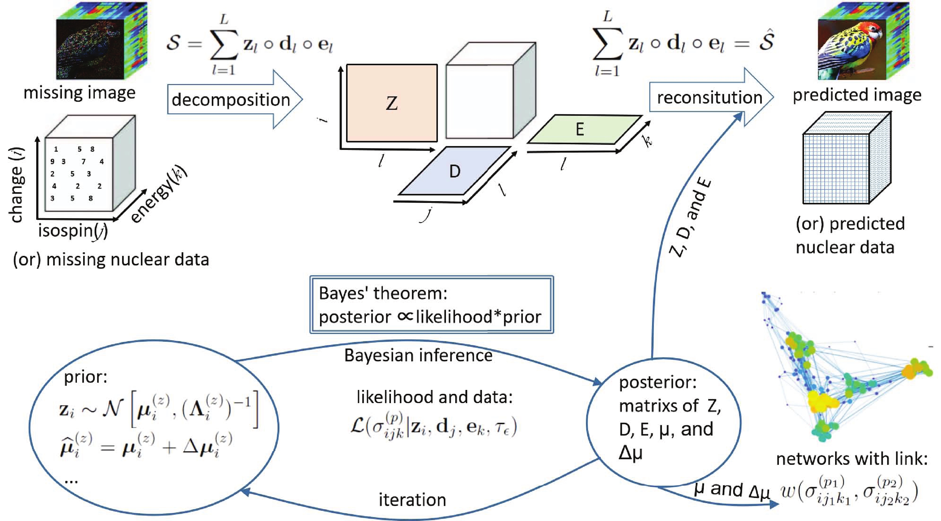 Figure1. (color?online)?Illustration for visualizing the definitions of the involved quantities and their relations.
 Figure2. (color online) Growth of nuclear reaction data and their evolving networks. Annual growth cross-section data of (a) (n,2n) reaction and (b) (γ,xn) reaction in the EXFOR database. Network generated from the (n,2n) cross-section data published before (c) 1960 and (d) 1965. The size and color of a node represent the degree
 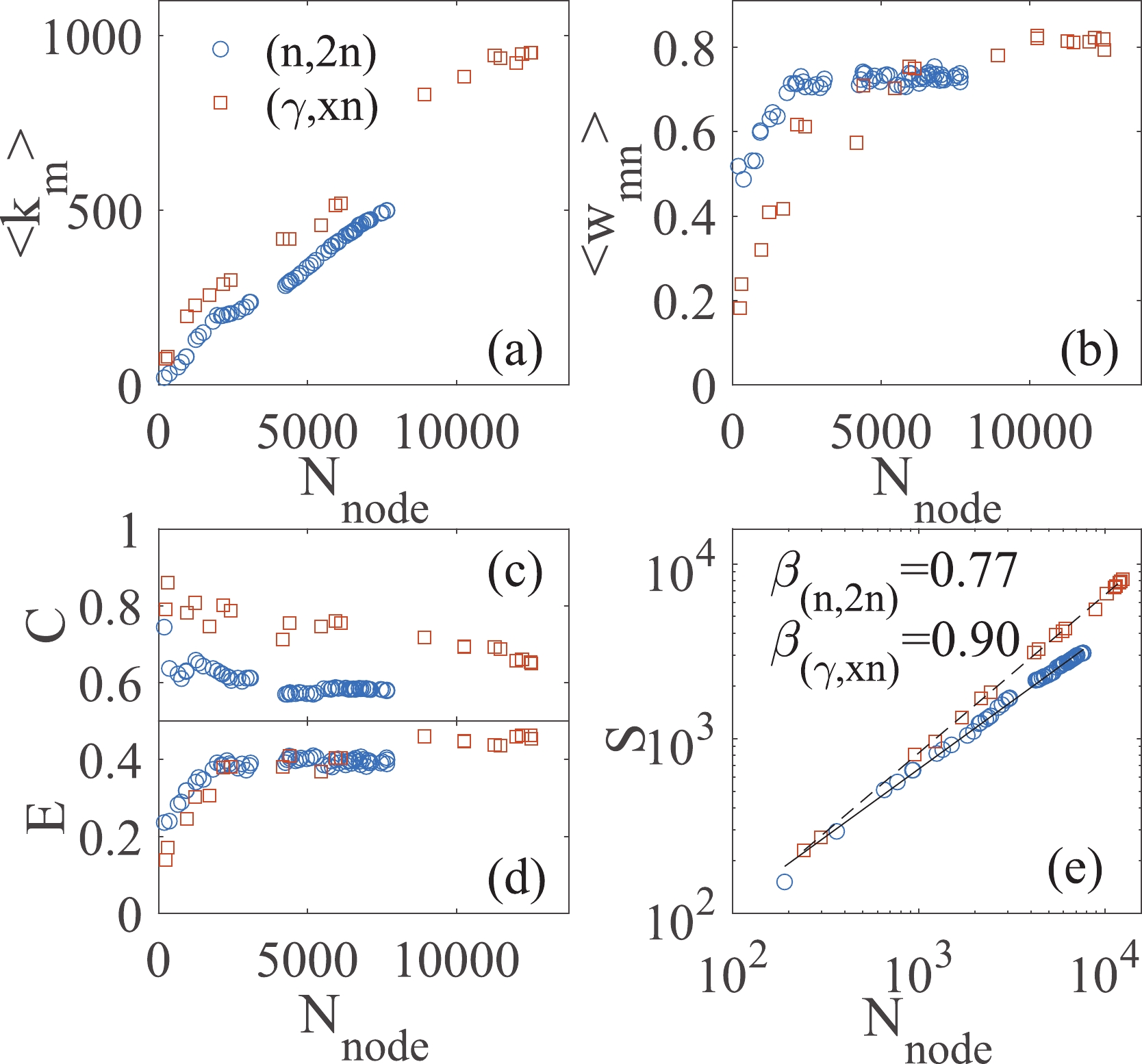 Figure3. (color?online)?Properties of the evolving small-world networks. (a) Mean degree of a node
 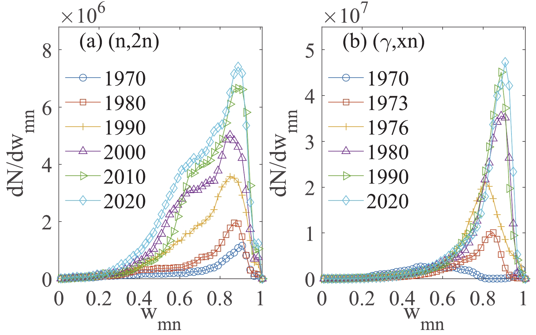 Figure4. (color?online)?Distribution of the edge-weight
  Figure5. (color?online)?Correlation between mean node weight
  Figure6. (color?online)?Distribution of the