Mengzhen Wang ^1,
, Yi Jiang ^2,
, Yinrui Liu ^2,
, Wenbin Qian ^2,
, Xiao-Rui Lyu ^2,
, Liming Zhang ^1,,
,

Corresponding author: Liming Zhang, liming.zhang@cern.ch

1.Center for High Energy Physics, Tsinghua University, Beijing 100084, China
2.University of Chinese Academy of Sciences, Beijing 100049, China
Received Date:2020-12-08
Available Online:2021-06-15
Abstract:In this study, the non-trival effect of the selection of reference particles for decay angle definitions is demonstrated when constructing the partial-wave amplitude of multi-body decays using helicity formalism. This issue is often ignored in the standard use case of helicity formalism. A new technique is proposed to test the selection of the particle ordering, and it can also be used as a generalized method to calculate the rotation operators that are used for the final-state alignment between different decay chains. Moreover, numerical validations are performed to support the arguments and to verify the effectiveness of the proposed technique.

HTML

--> --> -->

Partial-wave amplitude analysis is used extensively in experimental particle physics to understand the resonant structures in multi-body decays. Owing to the use of multi-dimensional phase-space variables, partial-wave amplitude analysis is more sensitive to the properties of resonant states than one-dimensional mass-spectrum analysis, and thus, it has become one of the most important techniques to explore exotic hadrons and to disentangle conventional contributions. Helicity formalism [1] is a popular technique for constructing the partial-wave amplitude. It sets a guideline to construct the angle-dependent amplitudes of two-body decays, which are further combined to form the amplitude of a decay chain (the cascade decay series that is made up of several two-body decays). The amplitudes of all of the decay chains are combined to form the total amplitude of the multi-body decays. When particles with non-zero spins are involved in the final state, a proper alignment of their spin axis should be created between different chains before the combination [2], so that the final states of different decay chains are defined consistently.
Helicity formalism was used in the amplitude analysis of the $ \Lambda_b^0\to \psi p K^- $ decay in the LHCb experiment, in which the first observation of pentaquarks was made [2]. An alternative method for the amplitude construction of a three-body decay, which is known as the Dalitz-Plot-Decomposition (DPD) approach, was proposed in Ref. [3], and has been proven to be equivalent to that used in the LHCb analysis [3]. However, numerical comparisons demonstrated an unexpected dependency between the consistency of these two formalisms and the selection of the reference particles when defining the two-body decay angles, which is termed the “particle ordering issue.” Inspired by this observation, further investigations are made on the general rule for the decay amplitude construction using helicity formalism.
The remainder of this paper is organized as follows. Sec. II briefly introduces puzzles in the standard helicity formalism and the influence on the decay amplitude. Sec. III proposes a systematic method based on the final-state alignment of different chains to derive the correct helicity amplitude. Sec. IV presents an example use case of the $ \Lambda_b^0 \to \psi p K^- $ amplitude analysis. For better clarification, the $ \Lambda_b^0 \to \psi p K^- $ three-body decay is used as an example throughout the text, but the discussions and conclusions should be valid for any other multi-body decays.

The total amplitude of the $ \Lambda_b^0 \to \psi p K^- $ decay is the sum of the amplitudes of the $ \Lambda^* $ chain, namely $ \Lambda_b^0 \to \psi \Lambda^*, \Lambda^* \to p K^- $, and the $ P_c $ chain, namely $ \Lambda_b^0 \to P_c K^-, P_c \to \psi p $ [2]. In standard helicity formalism [1], the amplitude for any two-body decay listed above, which is denoted as $ 0\to12 $, where 0, 1, and 2 indicate different particles, can be expressed as

$ A_{0\to12}(m_0, \theta_1, \phi_1) = H^{0\to12}_{\lambda_1, \lambda_2} D^{J_0}_{\lambda_0, \lambda_1-\lambda_2} (\phi_1, \theta_1, 0) R(m_0), $

(1)

where $ m_0 $ denotes the invariant mass of the two-body system, and $ J_0 $ is the spin of particle 0. The angles $ \theta_1 $ and $ \phi_1 $ represent the polar and azimuthal angles, respectively of the momentum of particle 1 defined in the rest frame of particle 0, as illustrated in Fig. 1, and are also known as the helicity angles of the $ 0\to12 $ two-body decay. Particle 1, the momentum of which is used to define the helicity angles, is hereafter denoted as the “reference particle” in this two-body decay. The label $ \lambda_i $ indicates the helicity of particle i, which is defined as its spin projection onto the momentum direction. The angle-dependent part of the amplitude is described using the Wigner D function $ D^{J_0}_{\lambda_0, \lambda_1-\lambda_2}(\phi_1, \theta_1, 0) $ [4], corresponding to a rotation operator transferring the spin axis from the initial stage^① to point to the momentum direction of particle 1. The mass-dependency is denoted as a line-shape function $ R(m_0) $, and the helicity coupling $ H^{0\to12}_{\lambda_1, \lambda_2} $, which is a constant complex number, is used to describe the decay dynamics.
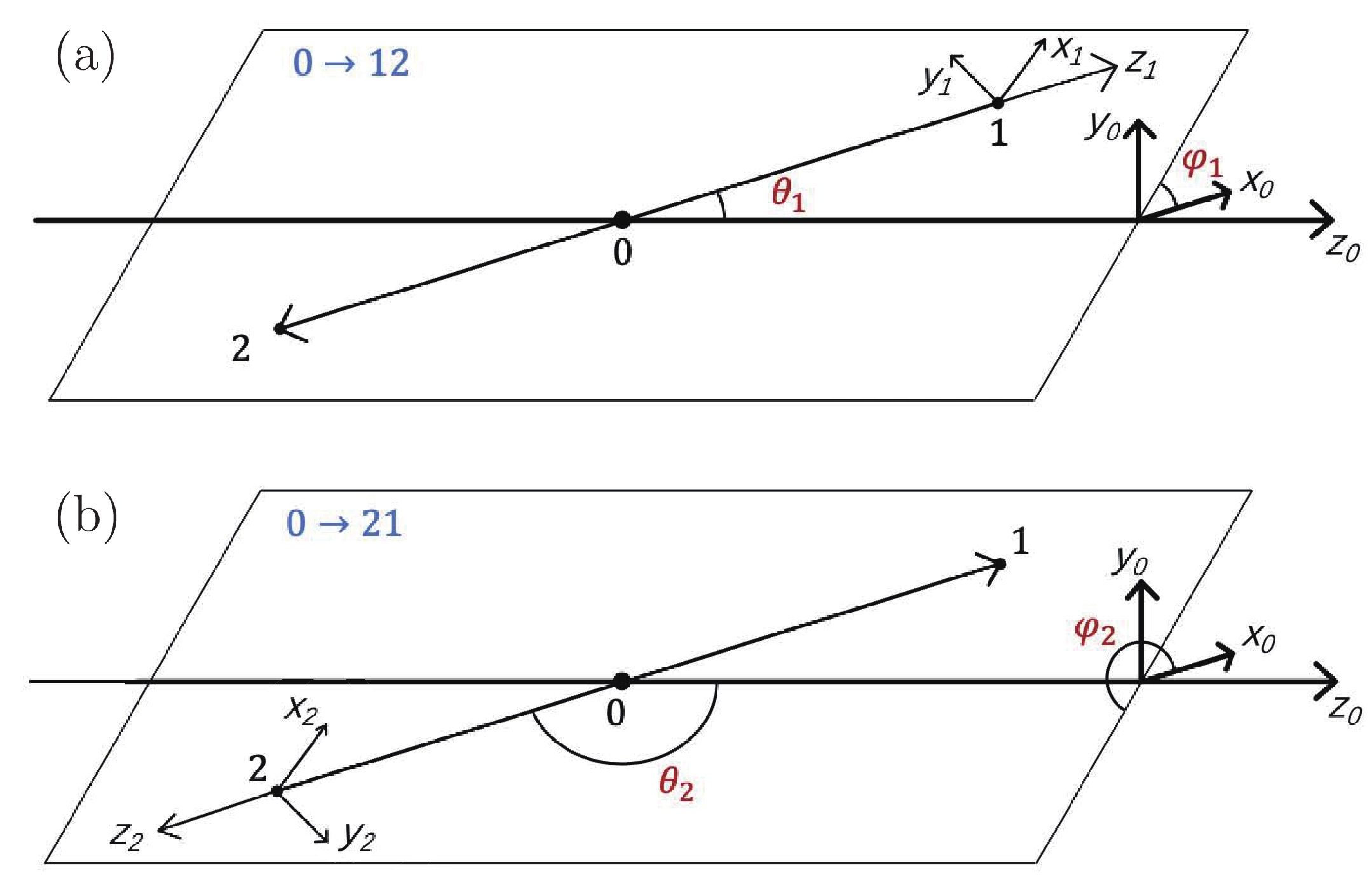Figure1. (color online) Helicity angles of $ 0\to12 $ decay (a) calculated based on momentum of particle 1, labeled as $ (\theta_1, \phi_1) $ or (b) calculated based on momentum of particle 2, labeled as $ (\theta_2, \phi_2) $.

The total amplitude of the $ \Lambda_b^0 \to \psi p K^- $ in Ref. [2] is constructed following the standard procedure of the helicity formalism construction. The decay amplitude of the $ \Lambda^* $ chain is the product of the amplitudes of the $ \Lambda_b^0 \to \psi \Lambda^* $ and $ \Lambda^* \to p K^- $ decays, and the decay amplitude of the $ P_c $ chain is the product of the amplitudes of the $ \Lambda_b^0 \to P_c K^- $ and $ P_c \to \psi p $ decays. An alignment term corresponding to a rotation of the final-state spin axis is added to the $ P_c $ chain amplitude prior to the combination of the two decay chains. Two potential defects remain in this standard procedure. The first one, which is denoted as the “particle ordering issue,” is how to select the reference particles in each two-body decay correctly. The second one, which is denoted as the “particle-two factor issue,” relates to the proper description of the evolution on the spin axis when the decay chain is connected using particles that are not taken as the reference of a two-body decay. These two issues are briefly mentioned in certain other papers, such as Refs. [3,5,6]. In this study, further discussions are provided to highlight the importance of these issues in both analytic and numerical approaches.
2

-->

A.Particle ordering issue

In standard helicity formalism, in principle, there is no preference regarding the selection of the reference particles. For the $ 0\to12 $ decay, one should be able to take either particle 1 or particle 2 as the reference. If particle 2 is selected, the angle-dependent part of the decay amplitude becomes $ D^{J_0}_{\lambda_0, \lambda_2-\lambda_1}(\phi_2, \theta_2, 0) $. As shown in Fig. 1, we have $ \theta_1 + \theta_2 = \pi $ and $ \phi_2 = \phi_2^\pm = \phi_1 \pm \pi $. The choice between $ \phi_2^+ $ and $ \phi_2^- $ depends on how the range of the $ \phi $ angles is defined. The most natural option is to define both $ \phi_1 $ and $ \phi_2 $ in the same region; for example, $ [-\pi, \pi) $, following which $ \phi_2^+ $ is taken when $ \phi_1<0 $, whereas $ \phi_2^- $ is taken when $ \phi_1>0 $. Given the properties of the Wigner D functions, we have

$ D^{J_0}_{\lambda_0, \lambda_1-\lambda_2}(\phi_1, \theta_1, 0) = (-1)^{J_0+\lambda_0 \pm \lambda_0} D^{J_0}_{\lambda_0, \lambda_2-\lambda_1}(\phi_2, \theta_2, 0) , $

(2)

and the difference in the angle-dependent amplitude when using different reference particles is a factor of $ f^{\pm} = (-1)^{J_0+\lambda_0 \pm \lambda_0} $, where $ f^+ $ is taken for decays with $ \phi_1<0 $, and $ f^- $ is taken for decays with $ \phi_1>0 $. If particle 0 is a meson, $ f^{\pm} = {(-1)}^{J_0} $ is simply a global factor that can be absorbed by the redefinition of helicity couplings. However, when particle 0 is a baryon, we have $ f^{+} = -f^- $. The value of $ f^{\pm} $ is different for events with $ \phi_1 > 0 $ or $ \phi_1 < 0 $. This minus sign has no effect on the module square of the amplitude of one decay chain. However, it becomes non-negligible when multiple decay chains are considered, as it directly influences the behaviour of the interference terms, and it is impossible to eliminate this phase-space-dependent factor by introducing any global terms that are shared by all of the events.
As an example, for the $ \Lambda_b^0 \to \psi p K^- $ amplitude analysis, the reference particle of the $ \Lambda^* \to p K^- $ decay is taken as the $ K^- $ particle in Ref. [2], and there is no particular reason for not taking the proton as the reference. Two possible settings of the reference particles involved in the $ \Lambda_b^0 \to \psi p K^- $ amplitude analysis are listed in Table 1, where “ordering 1” corresponds to the selection of the LHCb analysis [2], and “ordering 2” represents the nominal choice used in the DPD paper, which ensures that the decay planes for all of the decay chains are identical in the “aligned center-of-momentum frame” [3]. The only difference between these two orderings appears in the decay angle definition of the $ \Lambda^*\to p K^- $ decay, and as discussed above, they cannot both be correct without introducing corrections that are handled differently when $ \phi_{\Lambda^* \to p K^-} $ is larger or smaller than zero, where $ \phi_{\Lambda^* \to p K^-} $ is the azimuth decay angle of this two-body decay. The technique for implementing this type of correction is discussed later in Sec. V.

	Ordering 1	Ordering 2
$ \Lambda_b^0 \to \psi \Lambda^* $	$ \Lambda^* $	$ \Lambda^* $
$ \Lambda^* \to p K^- $	$ K^- $	p
$ \Lambda_b^0 \to P_c K^- $	$ P_c $	$ P_c $
$ P_c \to \psi p $	$ \psi $	$ \psi $

Table1.Selection of reference particles for each two-body decay involved in $ \Lambda_b^0 \to \psi p K^- $ amplitude analysis. Ordering 1 and ordering 2 correspond to the choices in Ref. [2] and Ref. [3], respectively.

The contributions of the estimated interference term between the amplitudes of the $ P_c $ and $ \Lambda^* $ chains, as a function of $ \phi_{\Lambda^* \to p K^-} $, calculated using standard helicity formalism under ordering 1 and ordering 2, are depicted in Fig. 2. When ordering 1 is used, an unphysical discontinuity is observed at $ \phi_{\Lambda^* \to p K^-} = 0 $, indicating a potential problematic issue, and the opposite behavior of the interference term when $ \phi_{\Lambda^* \to p K^-}>0 $ and $ \phi_{\Lambda^* \to p K^-}<0 $ leads to a significant cancellation of the interference contribution when integrating the full $ \phi_{\Lambda^* \to p K^-} $ regions, which can explain the zero interference contribution between the $ P_c $ and $ \Lambda^* $ chains observed in the ordering 1 configuration used in the LHCb analysis [2].
Figure2. Contribution from interference term between $ \Lambda^* $ and $ P_c $ chains as a function of $ \phi_{\Lambda^*\to p K^-} $, obtained using simulated $ \Lambda_b^0 \to \psi p K^- $ events. The left and right figures are based on particle ordering 1 and ordering 2, respectively.

In the DPD formula [3], the $ \phi $-angle related terms are shared by all of the decay chains; thus, it does not suffer from the potential non-global minus sign in the interference between different chains. A numerical comparison between the DPD formula and standard helicity formalism helps to understand which ordering is correct. The decay amplitudes using both formulas are calculated for each simulated event. As illustrated in Fig. 3, these two formulas are equivalent when ordering 2 is used. This also indicates that ordering 1 requires further treatment.
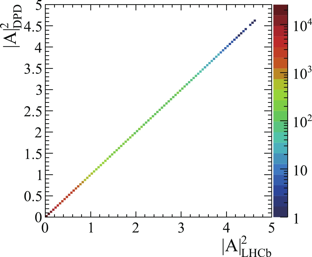Figure3. (color online) Two-dimensional distributions of amplitude module square of simulated $ \Lambda_b^0 \to \psi p K^- $ decays based on ordering 2. The x-axis represents the amplitude module square calculated using the formula in Ref. [2], whereas the y-axis is calculated using the DPD formula [3]. The mass-dependent terms and helicity couplings are generated randomly and are shared in the two formulas.

2 -->

B.Particle-two factor issue

In the DPD paper [3], the “Jacob-Wick particle-2 phase convention” was discussed, which was introduced in Ref. [6] and enables natural matching of the particle-2 helicity states to the canonical basis. In this section, the particle-2 phase convention is explained in an alternative method by introducing a “particle-two factor” to describe the transition of the spin axis appropriately. We also demonstrate that one must explicitly consider the particle-two phase factor to preserve the customary parity conservation relations,

$ H^{0\to12}_{-\lambda_1, -\lambda_2} = P_0 P_1 P_2 (-1)^{J_1 + J_2 - J_0} H^{0\to12}_{\lambda_1, \lambda_2}, $

(3)

where P represents the parity of the particles [2]. Moreover, there is a significant advantage in using the particle-two factor when multiple decay chains are added, as it ensures that the states are defined in the same phase convention. This does not occur directly if one simply takes the Jacob-Wick convention that treats the various particles asymmetrically.
The rotation operator indicated in Eq. (1) results in a spin axis along the same direction as the momentum of particle 1. However, to consider the further decay of particle 2, the commonly used initial spin axis is along the momentum direction of particle 2, which requires an additional term between the amplitudes of the $ 0\to1 2 $ process and further particle 2 decay. This additional term is known as the particle-two factor and is generally ignored in the standard procedure for constructing the helicity amplitude.
To obtain the exact form of the particle-two factor, we define a Cartesian coordinate system $ (x_1, y_1, z_1) $: as shown in Fig. 1, $ \vec{z}_1 $ and $ \vec{z}_2 $ are the momentum directions of particles 1 and 2, respectively, $ \vec{y}_1 $ is the normal vector of the $ 0\to12 $ decay plane, and $ \vec{x}_1 = \vec{y}_1 \times \vec{z}_1 $. A rotation operator corresponding to an angle of $ \pi $ along any axis in the $ x_1 - y_1 $ plane should be able to transfer the spin axis from $ \vec{z}_1 $ to $ \vec{z}_2 $. Different choices of the rotation axis result in different $ \vec{x}_2 $ and $ \vec{y}_2 $ axes, leading to varying definitions of the helicity angles of the particle 2 decay, which are calculated using the directions of $ \vec{z}_2 $, $ \vec{x}_2 $, and $ \vec{y}_2 $ as inputs [2]. A Wigner D function that corresponds to this rotation operator should be taken as the particle-two factor.
The most natural choice of the rotation axis is the $ \vec{x}_1 $ or $ \vec{y}_1 $ vector, both of which should be correct if the technique proposed in Sec. III is used. In Ref. [2], the $ \psi $ meson is not the reference particle in the $ \Lambda_b^0 \to \Lambda^* \psi $ decay and a rotation along the $ \vec{x}_1 $ axis is considered before calculating the $ \psi\to\mu^+\mu^- $ decay angles. The corresponding particle-two factor,

$ <J_2, -\lambda_2|R_x(\pi)|J_2, \lambda_2> = (-1)^{J_2}, $

(4)

is a constant parameter and can be absorbed into the definition of the helicity couplings. In this study, we suggest always taking the $ \vec{y}_1 $ axis as the rotation axis, which can prevent rolling over the decay planes to complicate the helicity amplitude construction. The corresponding particle-two factor is

$ <J_2, -\lambda_2|R_y(\pi)|J_2, \lambda_2> = d_{-\lambda_2, \lambda_2}^{J_2} = (-1)^{J_2 - \lambda_2}, $

(5)

where $ J_2 $ and $ \lambda_2 $ are the spin and helicity, respectively, of particle 2.
The particle-two factor is important for associating the helicity couplings and their $ LS $ representations properly, which is discussed in Ref. [3], and it is also essential for the parity determination of the resonant states, as demonstrated below. When particle 2 is a meson, this factor can be absorbed into the definition of the helicity coupling, namely $ H'^{0\to12}_{\lambda_1, \lambda_2} = (-1)^{J_2 - \lambda_2} H^{0\to12}_{\lambda_1, \lambda_2} $, and it generates no visible effect in the amplitude analysis. If particle 2 is a baryon, the effect on the parity conservation relation indicated in Eq. (3) becomes non-negligible. Under the parity transformation, the particle-two factor varies from $ (-1)^{J_2 - \lambda_2} $ to $ (-1)^{J_2 + \lambda_2} $, generating an additional minus sign. One cannot absorb the particle-two factor of a baryon into the definition of the corresponding helicity coupling, the behaviour of which under parity transformation would be otherwise modified, resulting in incorrect determinations of the particle parities.
If the further decay of particle 2 is not considered in the amplitude analysis, we suggest also adding the particle-two factor after the $ 0\to12 $ decay amplitude to manage all of the two-body decay amplitudes in a consistent manner. Otherwise, it acts as an additional term for the final-state alignment between the different chains.

As demonstrated in the previous section, the selection of the reference particle has a non-trival effect on the decay amplitude when fermions are involved in the decay process. This necessitates a guideline to make an appropriate selection or to add an additional term to the decay amplitude to cancel the non-global effect caused by switching the reference particles. Neither of these two features are well-described in the standard helicity formalism. A comparison between the standard helicity formalism and DPD formula [3] is a possible approach, but it is effective only for three-body decays and it does not uncover the nature of this issue. In this section, we attempt to solve this problem by investigating the final-state alignment between different decay chains.
In the $ \Lambda_b^0 \to \psi p K^- $ amplitude analysis [2], before the combination of the amplitude of the $ \Lambda^* $ and $ P_c $ chains, the spin state of the proton and muons should be properly aligned to be the same in different chains. A technique for correctly defining the spin state of the decay products was presented in Ref. [5], where the final spin states were obtained by carefully considering how they were associated with the initial spin state shared by all of the decay chains. In this study, we focus on the operators connecting the initial and final spin states, and propose an equation to define the correct final-state alignment in a mathematical manner, which can be used to validate whether the alignment is handled properly when ordering 1 or 2 is applied. It can also be used as a generalized method to determine the correct alignment term in the decay amplitude, once the selection of the reference particles is fixed.
The goal of the spin-axis alignment is to ensure that the combined $ \Lambda^* $ chain and $ P_c $ chain amplitudes are expressed to indicate the same initial and final states. With the proper alignment, the rotation operators that connect the initial and final spin states should be identical in the $ \Lambda^* $ and $ P_c $ chains. The mathematical description is

$ R_{{\rm{Euler}}, \Lambda^*} = B_{ P_c} B^{-1}_{ \Lambda^*} R_{{\rm{align}}, P_c} R_{{\rm{Euler}}, P_c} \;, $

(6)

where the subscripts $ \Lambda^* $ and $ P_c $ are used to denote two decay chains, and $ R_{\rm{Euler}} $ represents the cascade process of the Euler rotations that are associated with each two-body decay in the corresponding decay chain, with the Euler angles taken exactly from the decay angles in the amplitude. The symbol $ R_{\rm{align}} $ indicates the alignment rotation for a consistent final state definition between the $ P_c $ and $ \Lambda^* $ chains. Two boost operators, namely $ B_{P_c} $ and $ B^{-1}_{\Lambda^*} $, are involved to consider the difference between the reference frames under which the direction of the final spin axis is defined. The operator B represents the boost from the $ \Lambda_b^0 $ rest frame to that of the final-state particles through the intermediate resonances that are involved in each decay chain.
Once the particle ordering has been determined, the decay angles of all of the two-body decays can be calculated [1,2], based on which $ R_{\rm{Euler}} $ can be obtained. The boost operators can be calculated using the four-momentum information, and the alignment rotation becomes the only unknown part of Eq. (6). By solving Eq. (6) in either an analytic or a numerical manner, one can determine the correct alignment rotations. If the alignment angle has been determined using other approaches [2], Eq. (6) can also be used to validate whether the alignment is properly performed.
As all of the angles in Eq. (6) are directly obtained from the decay amplitude, it should be sensitive to the switching of the reference particles and should generate a visible effect once a proper representation is assigned to the rotation operators. For the $ \Lambda_b^0 \to \psi p K^-, \psi \to \mu^+ \mu^- $ amplitude analysis, the final-state particles related to the puzzles in Sec. II are all spin-half states. Therefore, in this study, the two-dimensional representation of the SU(2) group is used to describe the rotation operators. As the Wigner D function is the $ jm $ representation of the SU(2) group, this should be a good option for visualizing the properties in Eq. (2). The rotations along the z-axis, y-axis, and an arbitary axis labeled as $ \vec{a} $ are expressed using

$ {R_z}(\alpha ) = \left( {\begin{array}{*{20}{c}}{{{\rm e}^{-{\rm i}\alpha /2}}}&0\\0&{{{\rm e}^{{\rm i}\alpha /2}}}\end{array}} \right),$

(7)

$ {R_y}(\alpha ) = \left( {\begin{array}{*{20}{c}}{\cos (\alpha /2)}&{ - \sin (\alpha /2)}\\{\sin (\alpha /2)}&{\cos (\alpha /2)}\end{array}} \right), $

(8)

and

$ R(\alpha, \vec{a}) = R_z(\phi_a)R_y(\theta_a)R_z(\alpha)R_y(-\theta_a)R_z(-\phi_a), $

(9)

respectively, where $ \alpha $ represents the rotation angle, and $ \theta_a $ and $ \phi_a $ denote the polar and azimuthal angles of vector $ \vec{a} $, respectively. The corresponding representations of the boost operators, inspired by the $ (\dfrac{1}{2}, 0) $ representation of the Lorentz group [7], with a rapidity of $ \gamma $ along the z-axis and along any axis labeled as $ \vec{b} $, are

$ {B_z}(\gamma ) = \left( {\begin{array}{*{20}{c}} {{{\rm e}^{ - \gamma /2}}}&0\\ 0&{{{\rm e}^{\gamma /2}}} \end{array}} \right), $

(10)

and

$ B(\gamma, \vec{b}) = R_z(\phi_b)R_y(\theta_b)B_z(\gamma)R_y(-\theta_b)R_z(-\phi_b), $

(11)

respectively, where $ \theta_b $ and $ \phi_b $ are the polar and azimuthal angles of vector $ \vec{b} $.

In this section, an example is presented for the validation of the alignment of the proton spin axis between the $ P_c $ and $ \Lambda^* $ chains. Following the methodology of calculating both the decay angles and alignment angles in Ref. [2], the two options of reference particles listed in Table 1 are validated by verifying whether Eq. (6) is satisfied.
2

-->

A.Rotations when using ordering 1

If ordering 1 is used, the corresponding proton-related Euler rotation for the $ \Lambda^* $ chain is

$ \begin{aligned}[b] R_{{\rm{Euler}}, \Lambda^*} =& R(\pi, \vec{p}_{\Lambda^*}^{\Lambda_b^0} \times \vec{p}_{K}^{\Lambda^*}) R(\theta_{\Lambda^*}, \vec{p}_{\Lambda^*}^{\Lambda_b^0} \times \vec{p}_{K}^{\Lambda^*}) \\&\times R(\phi_K, \vec{p}_{\Lambda^*}^{\Lambda_b^0}) R(\theta_{\Lambda_b^0}, \vec{p}_{\Lambda^*}^{\Lambda_b^0} \times \vec{p}_{\Lambda_b^0}^{lab}) R(\phi_{\Lambda^*}, \vec{p}_{\Lambda_b^0}^{lab}) , \end{aligned} $

(12)

where $ \theta_{\Lambda_b^0} $ and $ \phi_{\Lambda^*} $ are the helicity angles of the $ \Lambda_b^0 \to \Lambda^* \psi $ decay, $ \theta_{\Lambda^*} $ and $ \phi_K $ are the helicity angles of the $ \Lambda^* \to p K^- $ decay [2], and the symbol $ \vec{p}_a^b $ denotes the momentum direction of particle a in the b rest frame. The rotation operator $ R(\theta_{\Lambda_b^0}, \vec{p}_{\Lambda^*}^{\Lambda_b^0} \times \vec{p}_{\Lambda_b^0}^{lab}) $$ R(\phi_{\Lambda^*}, \vec{p}_{\Lambda_b^0}^{lab}) $ corresponds to the helicity amplitude of the $ \Lambda_b^0 \to \Lambda^* \psi $ decay, and it transfers the spin axis from the direction of the $ \Lambda_b^0 $ momentum in the lab frame to that of the $ \Lambda^* $ momentum in the $ \Lambda_b^0 $ rest frame. The operator $ R(\pi, \vec{p}_{K}^{\Lambda^*}) R(\theta_{\Lambda^*}, \vec{p}_{\Lambda^*}^{\Lambda_b^0} \times \vec{p}_{K}^{\Lambda^*}) $ corresponds to the helicity amplitude of the $ \Lambda^* \to p K^- $ decay, and the direction spin axis is transfered along the direction of the $ K^- $ momentum in the $ \Lambda^* $ rest frame. An operator $ R(\pi, \vec{p}_{\Lambda^*}^{\Lambda_b^0} \times \vec{p}_{K}^{\Lambda^*}) $ is added, which corresponds to the particle-two factor described in Sec. IIB, as the proton is not the reference particle for the $ \Lambda^* \to p K^- $ decay angle definition. Similarly, for the $ P_c $ chain, the Euler rotation is

$ \begin{aligned}[b] R_{{\rm{Euler}}, {P}_{\rm{c}}} =& R(\pi, \vec{p}_{\psi}^{P_c} \times \vec{p}_{K}^{P_c}) R(\theta_{P_c}, \vec{p}_{\psi}^{P_c} \times \vec{p}_{K}^{P_c}) \\&\times R(\phi_\psi^{P_c}, \vec{p}_{P_c}^{\Lambda_b^0}) R(\theta_{\Lambda_b^0}^{P_c}, \vec{p}_{P_c}^{\Lambda_b^0} \times \vec{p}_{\Lambda_b^0}^{lab}) R(\phi_{P_c}, \vec{p}_{\Lambda_b^0}^{lab}), \end{aligned} $

(13)

where $ R(\theta_{\Lambda_b^0}^{P_c}, \vec{p}_{P_c}^{\Lambda_b^0} \times \vec{p}_{\Lambda_b^0}^{lab}) R(\phi_{P_c}, \vec{p}_{\Lambda_b^0}^{lab}) $ and $ R(\theta_{P_c}, \vec{p}_{\psi}^{P_c} \times \vec{p}_{K}^{P_c}) $$ R(\phi_\psi^{P_c}, \vec{p}_{P_c}^{\Lambda_b^0}) $ correspond to the helicity amplitude of the $ \Lambda_b^0 \to P_c K^- $ and $ P_c \to \psi p $ decays [2], respectively, and the spin axis is transfered from the same initial stage as that in the $ \Lambda^* $ chain, along the direction of the $ \psi $ momentum in the $ P_c $ rest frame. The operator $ R(\pi, \vec{p}_{\psi}^{P_c} \times \vec{p}_{K}^{P_c}) $ corresponds to the particle-two factor. The alignment rotation is expressed as

$ R_{{\rm{align}}, {\rm{P}}_{\rm{c}}} = R(\pi, \vec{p}_{K}^{\Lambda^*}) R(\theta_p, \vec{p}_{\psi}^{P_c} \times \vec{p}_{K}^{P_c}), $

(14)

corresponding to the alignment term between the $ \Lambda^* $ and $ P_c $ chains used in Ref. [2], where the alignment angle $ \theta_p $ is defined as the angle between the $ K^- $ and $ \psi $ particles in the proton rest frame and the value is restricted in $ \theta_p\in(0,\pi) $. When ordering 1 is used, the normal directions of the decay planes are opposite in the $ \Lambda^* $ and $ P_c $ chains; thus, an additional rotation $ R(\pi, \vec{p}_K^{\Lambda^*}) $, with an angle of $ \pi $ along the spin axis, is introduced to eliminate this difference.
2 -->

B.Rotations when using ordering 2

If ordering 2 is used, the Euler rotation for the $ \Lambda^* $ chain becomes

$ \begin{aligned}[b] R_{{\rm{Euler}}, \Lambda^*} =& R(\theta_{\Lambda^*}, \vec{p}_{\Lambda^*}^{\Lambda_b^0} \times \vec{p}_{p}^{\Lambda^*}) R(\phi_p, \vec{p}_{\Lambda^*}^{\Lambda_b^0})\\&\times R(\theta_{\Lambda_b^0}, \vec{p}_{\Lambda^*}^{\Lambda_b^0} \times \vec{p}_{\Lambda_b^0}^{lab})R(\phi_{\Lambda^*}, \vec{p}_{\Lambda_b^0}^{lab}). \end{aligned} $

(15)

The Euler rotation for the $ P_c $ chain becomes

$ \begin{aligned}[b] R_{{\rm{Euler}}, {P}_{\rm{c}}} =& R(\pi, \vec{p}_{\psi}^{P_c} \times \vec{p}_{K}^{P_c}) R(\theta_{P_c}, \vec{p}_{\psi}^{P_c} \times \vec{p}_{K}^{P_c}) \\&\times R(\phi_\psi^{P_c}, \vec{p}_{P_c}^{\Lambda_b^0}) R(\theta_{\Lambda_b^0}^{P_c}, \vec{p}_{P_c}^{\Lambda_b^0} \times \vec{p}_{\Lambda_b^0}^{lab}) R(\phi_{P_c}, \vec{p}_{\Lambda_b^0}^{lab}), \end{aligned} $

(16)

and the alignment rotation $R_{{\rm{align}}, {P}_{\rm{c}}}$ is

$ R_{{\rm{align}}, {P}_{\rm{c}}} = R(\theta_p, \vec{p}_{\psi}^{P_c} \times \vec{p}_{K}^{P_c}). $

(17)

The definitions of all of the angles are almost the same as that for ordering 1, except for $ \theta_{\Lambda^*} $ and $ \phi_p $, which are the $ \Lambda^* \to p K^- $ decay angles that are defined using the proton rather than the $ K^- $ particle as the reference. The rotation operator $ R(\pi, \vec{p}_{\psi}^{P_c} \times \vec{p}_{K}^{P_c}) $ corresponds to the particle-two factor mentioned in Sec. IIB.
2 -->

C.Boost operators

The boost operators are defined in the same manner for both ordering 1 and ordering 2. The operator $ B_{ \Lambda^*} $ first boosts the $ \Lambda_b^0 $ rest frame to the $ \Lambda^* $ rest frame and then to the proton rest frame; that is,

$ B_{ \Lambda^*} = B(-y_{p}^{\Lambda^*}, \vec{p}_{p}^{\Lambda^*}) B(-y_{\Lambda^*}^{\Lambda_b^0}, \vec{p}_{\Lambda^*}^{\Lambda_b^0}), $

(18)

where $ y_{a}^{b} $ represents the rapidity of particle a,

$ y = \frac{1}{2} \ln \left(\frac{E_a+p_a}{E_a-p_a}\right), $

(19)

which is defined in the rest frame of particle b. Similarly $B_{P_{\rm{c}}}$ first boosts the $ \Lambda_b^0 $ rest frame to the $ P_c $ rest frame and then to the proton rest frame; that is,

$ B_{P_{\rm{c}}} = B(-y_{p}^{P_c}, \vec{p}_{p}^{P_c}) B(-y_{P_c}^{\Lambda_b^0}, \vec{p}_{P_c}^{\Lambda_b^0}), $

(20)

2 -->

D.Validation of alignment equation

For improved visibility of the validation of Eq. (6), the distance between the matrices on its left and right sides is defined as

$ D = \sum\limits_{i,j} | L_{i,j}-R_{i,j}|^2 , $

(21)

where L represents the left side, namely $ R_{{\rm{Euler}}, \Lambda^*} $, whereas R indicates the right side, namely $B_{P_c} B_{\Lambda^*}^{-1} R_{{\rm{align}}, {P}_{\rm{c}}} R_{{\rm{Euler}}, {P}_{\rm{c}}}$, and the subscripts i and j are the row and column indexes for the L or R matrices, respectively. A distance D of zero indicates that L is equal to R. As both L and R are $ 2\times2 $ unitary matrices, when $ L = -R $, the distance becomes $ D = 8 $. Figure 4 depicts the distribution of D when all of the helicity and alignment angles are calculated using the method proposed in Ref. [2]. As illustrated in Fig. 4, the alignment is performed properly only for half of the events with $ \phi_{\Lambda^* \to p K^-} > 0 $ if ordering 1 is used, and for all of the events if ordering 2 is used. This is consistent with the numerical calculations discussed in Sec. IIA, and it demonstrates why ordering 2 is the correct choice.
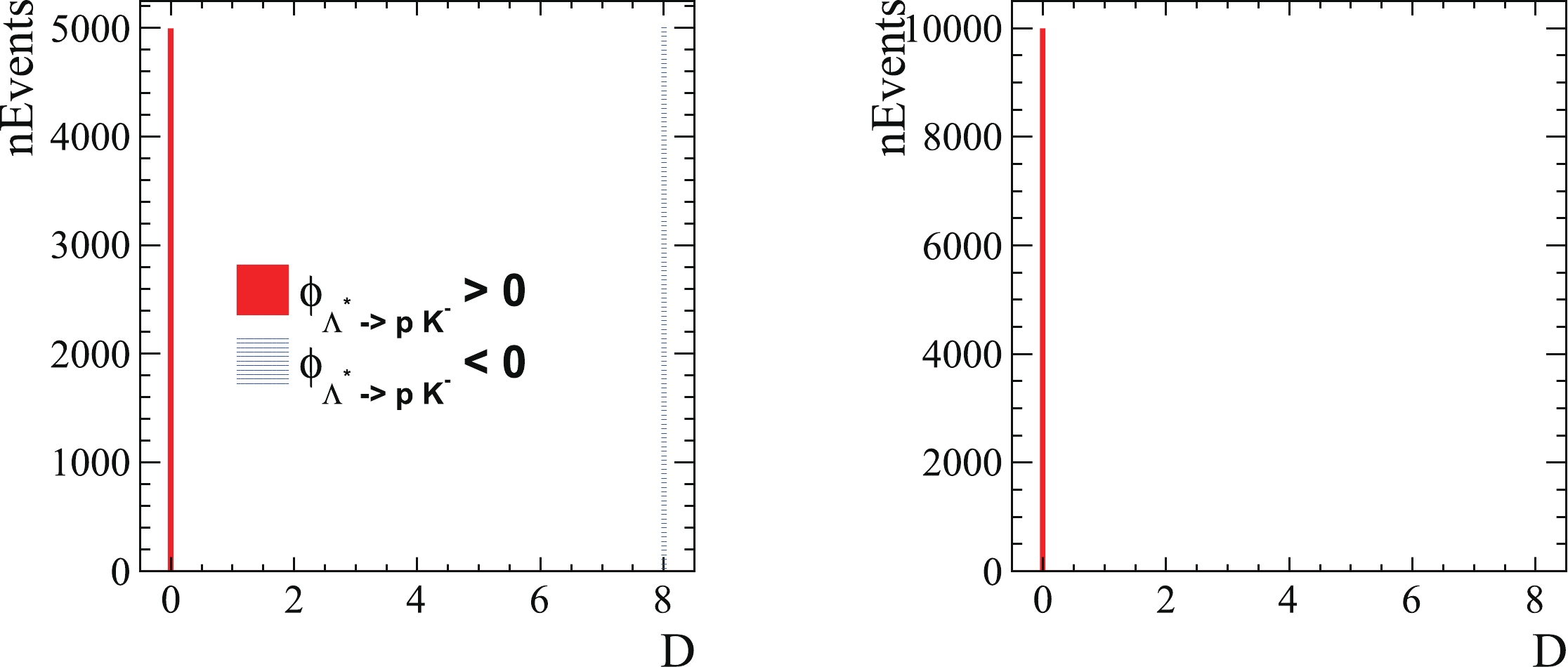Figure4. (color online) Distribution of D determined with helicity and alignment angles obtained using method proposed in Ref. [2]. The figure on the left is obtained based on ordering 1, where half of the candidates have perfect alignment between the two chains, whereas $ D = 8 $ for the other half, corresponding to a minus sign difference between the rotation matrices of the two chains. The figure on the right is obtained based on ordering 2, where all of the rotation matrices of the two chains are perfectly aligned for all of the generated events.

In the above discussions, the alignment angle $ \theta_p $ was fixed to the angle between the $ K^- $ and $ \psi $ momenta in the proton rest frame, and the validation was performed according to the particle orderings. Another use case exists in which the reference particles are determined and the correct alignment rotation formula can be obtained by solving Eq. (6). For example, if ordering 1 is used for the $ \Lambda_b^0 \to \psi p K^- $ amplitude analysis, the correct alignment rotation is exactly that in Eq. (14) for events with $ \phi_{\Lambda^*\to p K^-} > 0 $, as illustrated in Fig. 4. For the remaining events with $ D = 8 $, Eq. (14) is almost the correct solution, except for an additional minus sign. This can be solved by changing $ \theta_p $ to $ \theta_p + 2\pi $ for events with $ \phi_{\Lambda^*\to p K^-} < 0 $. This non-global $ 2\pi $ factor can recover the non-global minus sign that is introduced by the improper particle ordering mentioned in Sec. IIA.
For decays with more than three final-state particles, the alignment rotation obtained from Eq. (6) may be more complicated, and it needs to be expressed using both the polar and azimuthal angles. The rotation matrix should be transformed into the Euler style under a corresponding Cartesian coordinate system, which makes it easier to obtain the correct alignment term in the decay amplitude. Taking Fig. 1 as an example, consider the alignment of particle 1. The Euler angles should be calculated in the $ (x_1, y_1, z_1) $ system and the Euler rotation for the spin-axis alignment can be expressed as

$ R_{z_1}(\alpha) R_{y_1}(\beta) R_{z_1}(\gamma), $

(22)

The direction of $ \vec{x}_1, \vec{y}_1 $, and $ \vec{z}_1 $ can be derived using the four momentum information [2], based on which the Euler rotation connecting the $ (x_1, y_1, z_1) $ and $ (x, y, z) $ frames can be obtained, which is labeled as $ R_{{\rm{Euler}}, {\rm{trans}}} $. Subsequently, we have

$ R_{z_1}(\alpha) R_{y_1}(\beta) R_{z_1}(\gamma) = R_{{\rm{Euler}}, {\rm{trans}}} R_{z}(\alpha) R_{y}(\beta) R_{z}(\gamma) R^{-1}_{{\rm{Euler}}, {\rm{trans}}} $

(23)

and

$ {R_z}(\alpha ){R_y}(\beta ){R_z}(\gamma ) = \left( {\begin{array}{*{20}{c}}\!\!\!\!{{{\rm e}^{-{\rm i}(\alpha + \gamma )/2}}\cos (\beta /2)}&{ - {{\rm e}^{-{\rm i}(\alpha - \gamma )/2}}\sin (\beta /2)}\!\!\!\!\\\!\!\!\!{{{\rm e}^{{\rm i}(\alpha - \gamma )/2}}\sin (\beta /2)}&{{{\rm e}^{{\rm i}(\alpha + \gamma )/2}}\cos (\beta /2)}\!\!\!\!\end{array}} \right).$

(24)

If the alignment rotation obtained from Eq. (6) is

$ {R_{{\rm{Euler}}}} = \left( {\begin{array}{*{20}{c}}a&b\\c&d\end{array}} \right), $

(25)

we can translate it into

$ R_{{\rm{Euler}},{\rm{trans}}}^{ - 1}{R_{{\rm{Euler}}}}{R_{{\rm{Euler}},{\rm{trans}}}} = \left( {\begin{array}{*{20}{c}}{a'}&{b'}\\{c'}&{d'}\end{array}} \right),$

(26)

and the Euler angles for the alignment term can be determined using the following relations:

$ \begin{aligned}[b] \cos(\beta/2) =& |a'| , \sin(\beta/2) = |b'|, \\ \alpha+\gamma =& -2{\rm{Arg}}(a'), \\ \alpha-\gamma =& 2{\rm{Arg}}(c'). \end{aligned}$

(27)

Given the preceeding discussions, we suggest several modifications to the $ \Lambda_b^0 \to \psi p K^- $ decay amplitude with respect to that used in Ref. [2], based on either ordering 1 or ordering 2.
If ordering 2 is used, the modifications are as follows:
● For the $ \Lambda^*\to p K^- $ decay, use the proton as the reference particle.
● Add the particle-two factors in the decay amplitude, including the term of $ (-1)^{J_p - \lambda_p} $ to the $ P_c $ chain amplitude and the term of $ (-1)^{J_{\psi} - \lambda_{\psi}} $ to the $ \Lambda^* $ chain amplitude. As noted in Sec. IIB, the suggested rotation axis for considering the particle-two factor in this study differs from that used in Ref. [2]; thus, the decay angles of the $ \psi\to\mu^+\mu^- $ process in the $ \Lambda^* $ chain should be modified accordingly, where the $ \phi $ angle should be changed to $ \phi+\pi $ when $ \phi<0 $ and $ \phi-\pi $ when $ \phi>0 $. The modification of the $ \phi $ angle definition is simply for consistency and will not influence the major results of the amplitude analysis, as the additional $ \pm \pi $ phase only contributes to a global minus sign in the $ \Lambda^* $ chain amplitude [2].
If ordering 1 is used, the modifications are as follows:
● For events with $ \phi_{\Lambda^*\to p K^-} < 0 $, change the alignment angle $ \theta_p $ to $ \theta_p + 2\pi $
● The operator $ R(\pi, \vec{p}_K^{\Lambda^*}) $ in Eq. (14) should also be considered as part of the alignment rotation. The alignment term between the $ P_c $ and $ \Lambda^* $ chains should be changed from $ d_{\lambda_p, \lambda'_p}^{\frac{1}{2}}(\theta_p) $ to $ D_{\lambda_p, \lambda'_p}^{\frac{1}{2}}(\pi,\theta_p,0) $.

Partial-wave amplitude analysis plays an important role in investigating the properties of the resonant structures in multi-body decays. Helicity formalism, which is a widely-used technique for constructing the decay amplitude, has been adopted to discover or precisely measure the properties of both exotic and conventional resonant states. However, the principle of selecting the reference decay product when calculating the helicity angles of two-body decays, namely the particle ordering issue, has not often been discussed in the traditional use of helicity formalism.
In this study, we first demonstrated the necessity of carefully considering the particle ordering issue, particularly for decays involving spin-half-integral particles, where the selection of the reference particles has a non-negligible influence on the interference term. Thereafter, we proposed a new technique to validate whether the decay amplitude is expressed correctly under a dedicated particle ordering. This technique verifies whether the rotation operators involved in different decay chains properly align the spin axes of the final-state particles. A dedicated representation for the operators has been proposed, which can aid experimentalists in conducting event-by-event checking of the final-state alignment in a numerical manner. Using this new technique, a proper final-state alignment can be achieved with any given particle orderings, and the inconsistency between different orderings can be cancelled by assigning different alignment rotation operators. Numerical calculations using the simulated $ \Lambda_b^0 \to \psi p K^- $ decays [2] have also been presented as an example. The technique proposed in this article contributes to the ongoing and future particle-wave amplitude analysis of decays with baryons, for example, $ \Lambda_c^+ \to p K^- \pi^+ $, $ \Lambda_b^0 \to D^0 p \pi^- $, $ B^0\to D^0 p \bar{p} $, and $ \psi(2S) \to $$ \eta p \bar{p} $, to construct the decay amplitude correctly.

We thank Mikhail Mikhasenko and Tomasz Skwarnicki for their valuable discussions on the Dalitz-plot decomposition formalism, which inspired the observation of the particle ordering issue and motivated us to investigate helicity formalism further, and also for highlighting the Jacob-Wick particle-2 phase convention in the amplitude analysis. We thank Andy Beiter, Chen Chen, Mikhail Mikhasenko, Alessandro Pilloni, César Fernández Ramírez, Adam Szczepaniak, Tomasz Skwarnicki, Zhihong Shen, and Zehua Xu for their discussions on helicity formalism.