


HTML
--> --> -->In particular, multi-doublet Higgs models are a straightforward extension of the SM, in which the total vacuum expectation value (VEV) is given by
Furthermore, supersymmetry (SUSY) has been studied extensively as a possibility to solve, or at least to ameliorate, the hierarchy problem [13]. The minimal SUSY model (MSSM) includes two Higgs doublets and its structure is such that each doublet couples to only one fermion type, and thus, FCNCs are not allowed in the model. The next multi-doublet SUSY Higgs model must include four Higgs doublets, where each doublet is denoted as
In this study, we consider a four-Higgs doublet SUSY model with a more restricted parameter space, which is achieved by considering a version of the model of the "private type." This model is defined by requiring that one doublet gives masses to each fermion type, namely,
The goal of this study is to construct this private SUSY Higgs model, and to derive the interactions of the Higgs boson with gauge bosons and fermions. Moreover, we aim to identify regions of the parameter space that are consistent with high-energy data on the Higgs couplings, as derived from the LHC. As FCNCs only occur in the up-type quark sector in our model, the constraints from low-energy flavor physics would need to be considered; however, these are rather mild. In fact, the LHC data on Higgs couplings to gauge bosons and fermions (including FCNC top decay
The remainder of this paper is organized as follows. In Section II, we review the model construction, including the Higgs potential (for this, we closely follow Ref. [19]), and then, we perform the minimization of the Higgs potential (V) and derive the scalar mass matrices; we also present an approximate diagonalization of the
2
A.Model superpotential
The starting point when studying the Higgs and Yukawa sectors in a supersymmetric model is to describe the corresponding superpotential. This model includes four Higgs chiral superfields, each of which includes both the scalar and fermion components, namely the Higgses and Higgsinos. Owing to the anomaly cancellation, two of these, $ W = W_{\rm Yuk} + \sum\limits_i [ \mu_ {i1} \hat{H}_{ui} \cdot \hat{H}_{d} + \mu_ {i2} \hat{H}_{ui} \cdot \hat{H}_{l}]. $  | (1) |
In turn, the form of the Yukawa superpotential (
$ \begin{aligned}[b] W_{\rm Yuk} =& [ \hat{Q} Y_{u1} \hat{H}_{u1} \hat{U} + \hat{Q} Y_{u2} \hat{H}_{u2} \hat{U}] \\& + \hat{Q} Y_ {d} \hat{H}_d \hat{D} + \hat{L} Y_l \hat{H}_{l} \hat{E}. \end{aligned}$  | (2) |
  |   |   | Q | L | |
  |   | + | + | + | + |
  | + |   | + | + | + |
  |   | + |   | + | + |
Table1.Discrete symmetries for our SUSY 4HDM.
The power of these discrete symmetries is such that it permits the classification of different types of multi-Higgs models. For example, when considering a two-Higgs doublet model (2HDM), one can discuss types I, II, or III; in this model, both doublets
The discrete symmetries may cause some of the μ-terms to vanish. Furthermore, these discrete symmetries may be imposed on the soft-breaking terms. Thus, the question arises as to whether the resulting Higgs spectrum is viable, namely one can have a light SM-like Higgs boson with
2
B.Higgs potential of SS-4HDM
In this section, we discuss the general Higgs potential for the supersymmetric model with four Higgs doublets, following the notation of Ref. [19]. After discussing the minimization conditions, the general form of the Higgs mass matrices is derived.The Higgs doublets are the scalar components of the Higgs chiral multiplets, and are written as follows:
$ \begin{aligned}[b]& {H_{ui}} = \left( {\begin{array}{*{20}{c}}{H_{ui}^ + }\\{H_{ui}^0}\end{array}} \right)(i = 1,2),\\&{H_d} = \left( {\begin{array}{*{20}{c}}{H_d^0}\\{H_d^ - }\end{array}} \right),\\&{H_l} = \left( {\begin{array}{*{20}{c}}{H_l^0}\\{H_l^ - }\end{array}} \right), \end{aligned}$  | (3) |
$ H^0_k = \frac{1}{\sqrt{2}}(v_k+\eta_k+i\chi_k)\;\;\;\;{\rm{and}}\;\;\;\;(k = u_1,d,l,u_2). $  | (4) |
As demonstrated in [19, 20], the scalar potential of the Higgs fields takes the following form:
$ \begin{aligned}[b]V =& \sum\limits_{i = 1}^2\bigg((|\mu_{i1}|^2+|\mu_{i2}|^2+\tilde{m}_{ui}^2)(|H_{ui}^0|^2+|H_{ui}^+|^2)+(|\mu_{1i}|^2+|\mu_{2i}|^2+\tilde{m}_{di}^2)(|H_{di}^0|^2+|H_{di}^+|^2)\bigg)\\&+ \bigg((\mu_{11}^*\mu_{21}+\mu_{12}^*\mu_{22})(H_{u1}^{0*}H_{u2}^{0}+H_{u1}^{+*}H_{u2}^{+})+(\mu_{11}^{*}\mu_{12}+\mu_{21}^{*}\mu_{22})(H_{d1}^{0*}H_{d2}^{0}+H_{d1}^{-*}H_{d2}^{-})+c.c\bigg)\\ &+\Bigg(\sum\limits_{i = 1}^{2}\sum\limits_{j = 1}^{2}b^2_{ij}(H_{ui}^{+}H_{dj}^{-}-H_{ui}^{0}H_{dj}^{0})+c.c.\Bigg)+\frac{g^2+g'^2}{8}\Bigg(\sum\limits_{i = 1}^{2}(|H_{ui}^{0}|^2+|H_{ui}^{+}|^2-|H_{di}^{0}|^2+|H_{di}^{-}|^2)\Bigg)^2\\ &+\frac{g^2}{2}\bigg(\sum\limits_{i = 1}^{2}|(H_{ui}^{+*}H_{ui}^{0}+H_{di}^{0*}H_{di}^{-})|^2-\sum\limits_{i = 1}^{2}\sum\limits_{j = 1}^{2}(|H_{ui}^{0}|^2-|H_{di}^{0}|^2)(|H_{uj}^{+}|^2-|H_{dj}^{-}|^2)\bigg), \end{aligned} $  | (5) |
$ v_{1} = \frac{\sqrt{2}M_Z}{\sqrt{(g^2+g'^2)(1+\tan^2\omega)}}\cos\beta, $  | (6) |
$ v_{4} = \frac{\sqrt{2}M_Z}{\sqrt{(g^2+g'^2)(1+\tan^2\omega)}}\tan\omega\sin\alpha, $  | (7) |
$ v_d = \frac{\sqrt{2}M_Z}{\sqrt{(g^2+g'^2)(1+\tan^2\omega)}}\sin\beta, $  | (8) |
$ v_l = \frac{\sqrt{2}M_Z}{\sqrt{(g^2+g'^2)(1+\tan^2\omega)}}\tan\omega\cos\alpha. $  | (9) |
$ \Delta_{u_1}+\left(\mu _{11} \mu _{21}+\mu _{12} \mu _{22}\right)c^{-1}_\beta s_\alpha t_\omega - b^2_{12}c^{-1}_\beta c_\alpha t_\omega- b^2_{11} t _\beta+\frac{1}{4}{{Mz}}^2\left(c_{2 \beta}c^2_\omega -c_ {2 \alpha}s ^2_\omega\right) = 0, $  | (10) |
$ \Delta_d+\left(\mu _{11} \mu _{12}+\mu _{21} \mu _{22}\right)s^{-1}_\beta c_\alpha t_\omega-b^2_{21}s^{-1}_\beta s_\alpha t_\omega- b^2_{11}t^{-1}_\beta+\frac{1}{4}{{Mz}}^2 \left( c_{2 \alpha} s ^2_\omega -c_{2\beta}c ^2_\omega\right) = 0, $  | (11) |
$ \Delta_l - b^2_{21}s_\beta t^{-1}_\omega s^{-1}_\alpha+ \left(\mu _{11} \mu _{21}+\mu _{12} \mu _{22}\right)c_\beta t^{-1}_\omega s^{-1}_\alpha-b^2_{22}t^{-1}_ \omega s^{-1}_\alpha c_\alpha+\frac{1}{4}{{Mz}}^2 s_\omega\left[c_{2\beta} c_\omega-c_{2\alpha} s_\omega\right] = 0, $  | (12) |
$ \Delta_{u_2} - b^2_{12}c_\beta c^{-1}_\alpha t^{-1}_\omega-(\mu_{11}\mu_{12}+\mu_{21}\mu_{22})s_\beta c^{-1}_\alpha t^{-1}_\omega-t_\alpha t^{-1}_\omega b^2_{22}+\frac{1}{4}{{Mz}}^2\left[c_{2\alpha}s^2_\omega-c_{2\beta}c^2_\omega\right] = 0, $  | (13) |
2
C.Higgs mass matrices
We consider the CP-invariant case and focus on the neutral CP-even Higgs fields, which are obtained from the real parts of the neutral components. In the basis ( $ {{\cal{M}}^2} = \left( {\begin{array}{*{20}{c}}{m_{{u_1}{u_1}}^2}&{m_{{u_1}d}^2}&{m_{{u_1}l}^2}&{m_{{u_1}{u_2}}^2}\\{m_{d{u_1}}^2}&{m_{dd}^2}&{m_{dl}^2}&{m_{{u_2}d}^2}\\{m_{l{u_1}}^2}&{m_{ld}^2}&{m_{ll}^2}&{m_{{u_2}l}^2}\\{m_{{u_2}{u_1}}^2}&{m_{{u_2}d}^2}&{m_{{u_2}l}^2}&{m_{{u_2}{u_2}}^2}\end{array}} \right), $  | (14) |
$ m^2_{u_1u_1} = \frac{1}{2}\Delta_{u1}+\frac{1}{8}m_Z^2\left((2 \cos2\beta+1)\cos ^2\omega-\cos2\alpha\sin ^2\omega \right), $  | (15) |
$ m^2_{u_1 d} = -\frac{1}{2} b^2_{11}-\frac{1}{2}m_Z^2\sin 2\beta \cos ^2\omega, $  | (16) |
$ m^2_{u_1l} = \frac{1}{2}\left(\mu_{11} \mu _{21}+\mu _{12}\mu _{22}\right)+\frac{1}{2}m_Z^2\cos\beta\sin\alpha \sin 2\omega, $  | (17) |
$ m^2_{dd} = \frac{1}{2}\Delta_d+\frac{1}{8}m_Z^2 \left((1-2 \cos2 \beta) \cos ^2\omega+\cos 2 \alpha \sin ^2\omega\right), $  | (18) |
$ m^2_{dl} = -\frac{1}{2}b^2_{21}-\frac{1}{2} m_Z^2\sin\alpha\sin\beta\sin 2\omega, $  | (19) |
$ m^2_{ll} = \frac{1}{2}\Delta_l+ \frac{1}{8}m_Z^2\left((1-2 \cos 2\alpha) \sin ^2\omega+\cos 2\beta\cos ^2\omega\right), $  | (20) |
$ m_{u_2u_2}^2 = \frac{1}{2}\Delta_{u_2}+\frac{1}{8}m_Z^2\left((2\cos{2\alpha}+1)\sin^2\omega-\cos{2\beta} \cos^2\omega\right), $  | (21) |
$ m_{u_2u_1}^2 = -\frac{1}{2}b^2_{12}-\frac{1}{2}m_Z^2\cos\alpha\cos\beta\sin 2\omega, $  | (22) |
$ m_{u_2 d}^2 = \frac{1}{2}(\mu_{11}\mu_{12}+\mu_{21}\mu_{22})+\frac{1}{2}m_Z^2\cos\alpha\sin\beta\sin 2\omega, $  | (23) |
$ m_{u_2 l}^2 = -\frac{1}{2}b^2_{22}-\frac{1}{2}m_Z^2\sin 2\alpha \sin^2\omega. $  | (24) |
2
D.Approximate diagonalization
We assume that the $ {\cal{M}}^2\approx \left( {\begin{array}{*{20}{c}}{m_{{u_1}{u_1}}^2}&{m_{{u_1}d}^2}&{m_{{u_1}l}^2}&{{\epsilon_1}}\\{m_{d{u_1}}^2}&{m_{dd}^2}&{m_{dl}^2}&{{\epsilon_2}}\\{m_{l{u_1}}^2}&{m_{ld}^2}&{m_{ll}^2}&{{\epsilon_3}}\\{{\epsilon_1}}&{{\epsilon_2}}&{{\epsilon_3}}&{m_{{u_2}{u_2}}^2}\end{array}} \right).$  | (25) |
$ \left( {\begin{array}{*{20}{c}}{{h_1}}\\{{h_2}}\\{{h_3}}\\{{h_4}}\end{array}} \right) = O({\delta _i})\left( {\begin{array}{*{20}{c}}{{\eta _1}}\\{{\eta _d}}\\{{\eta _l}}\\{{\eta _2}}\end{array}} \right),$  | (26) |
$ {\cal{M}}^2 = {O^T}({\delta _i})\left( {\begin{array}{*{20}{c}}{m_{{h_1}}^2}&0&0&0\\0&{m_{{h_2}}^2}&0&0\\0&0&{m_{{h_3}}^2}&0\\0&0&0&{m_{{h_4}}^2}\end{array}} \right)O({\delta _i}). $  | (27) |
$ {O^T}({\delta _i}) \!=\! \left(\!\! {\begin{array}{*{20}{c}}\!\!{{c_{{\delta _1}}}{c_{{\delta _2}}}}\!\!&\!\!{ - {c_{{\delta _3}}}{s_{{\delta _1}}} - {c_{{\delta _1}}}{s_{{\delta _2}}}{s_{{\delta _3}}}}\!\!&\!\!{{s_{{\delta _1}}}{s_{{\delta _3}}} - {c_{{\delta _1}}}{c_{{\delta _3}}}{s_{{\delta _2}}}}\!\!&\!\!0\!\!\\\!\!{{c_{{\delta _2}}}{s_{{\delta _1}}}}\!\!&\!\!{{c_{{\delta _1}}}{c_{{\delta _3}}} - {s_{{\delta _1}}}{s_{{\delta _2}}}{s_{{\delta _3}}}}\!\!&\!\!{ - {c_{{\delta _3}}}{s_{{\delta _1}}}{s_{{\delta _2}}} - {c_{{\delta _1}}}{s_{{\delta _3}}}}\!\!&\!\!0\!\!\\\!\!{{s_{{\delta _2}}}}\!\!&\!\!{{c_{{\delta _2}}}{s_{{\delta _3}}}}\!\!&\!\!{{c_{{\delta _2}}}{c_{{\delta _3}}}}\!\!&\!\!0\!\!\\0\!\!&\!\!0\!\!&\!\!0\!\!&\!\!1\end{array}} \!\!\right). $  | (28) |
$ \eta_1 = c_{\delta _1}c_{\delta _2}h_1 -(c_{\delta _3 }s_{\delta _1}+c_{\delta _1}s_{\delta _2}s_{\delta _3} )h_2+ (s_{\delta _1}s_{\delta _3}-c_{\delta _1}c_{\delta _3} s_{\delta _2} )h_3, $  | (29) |
$ \eta_d = c_{\delta _2}s_{\delta _1}h_1 +(c_{\delta _1}c_{\delta _3}-s_{\delta _1}s_{\delta _2}s_{\delta _3})h_2 -(c_{\delta _3}s_{\delta _1}s_{\delta _2}+c_{\delta _1}s_{\delta _3})h_3, $  | (30) |
$ \eta_l = s_{\delta _2}h_1 +c_{\delta _2}s_{\delta _3}h_2 +c_{\delta _2}c_{\delta _3}h_3, $  | (31) |
$ \eta_4 = h_4. $  | (32) |
2
E.Higgs boson spectrum
At this point, we should verify that the resulting Higgs spectrum is viable, namely that we have a light SM-like Higgs boson with $\begin{aligned}[b]m^2_{h}=& \frac{m_Z^2}{8} F(\alpha, \beta, \delta_i, \omega) - s_{\delta_1} c_ {\delta_1} c^2_{\delta_2} b^2_{11} - s_{\delta_1} s_{\delta_2} c_{\delta_2} b^2_{21} \\ &+\frac{1}{2} \tilde{m}_{u_1}^2 c^2_{\delta_1} c^2_{\delta_2}+\frac{1}{2} \tilde{m}_d^2 s^2_{\delta_1} c^2_{\delta_2}+\frac{1}{2} \tilde{m}_l^2 s^2_{\delta_2}\\& +\frac{3G_F}{\sqrt{2}\pi^2}\frac{m_t^4}{r_{1u}}\log\frac{m^2_{\rm stop}}{m^2_t}, \end{aligned}$  | (33) |
$ \begin{aligned}[b] F (\alpha, \beta, \delta_i, \omega) = & \left[ \right. c^2_{\delta_1} c ^2_{\delta_2} \left( (2 c_{ 2 \beta} +1) c^2_{\omega} - c_{ 2 \alpha} s^2_\omega \right) \\&+ s ^2_{\delta_1} c ^2_{\delta_2} \left( c_{ 2 \alpha} s ^2_\omega +(1-2 c_{ 2 \beta} ) c ^2_\omega\right) \\& +s ^2_{\delta_2} \left( (1-2 c_{ 2 \alpha} ) s ^2_\omega +c_{ 2 \beta} c^2_\omega \right) \\ &+c_ \beta c_{\delta_1} \left( s_{\alpha} s_{ 2 \delta_2} s_{ 2 \omega} - 4 s_ {\beta} s_{\delta_1} c ^2_{\delta_2}c ^2_\omega \right) \\& -4 s_\alpha s_\beta s_{\delta_1} s_{\delta_2} c_{\delta_2} s_\omega c_\omega \left.\right]. \end{aligned}$  | (34) |
Then, in Fig. 1(a) we show
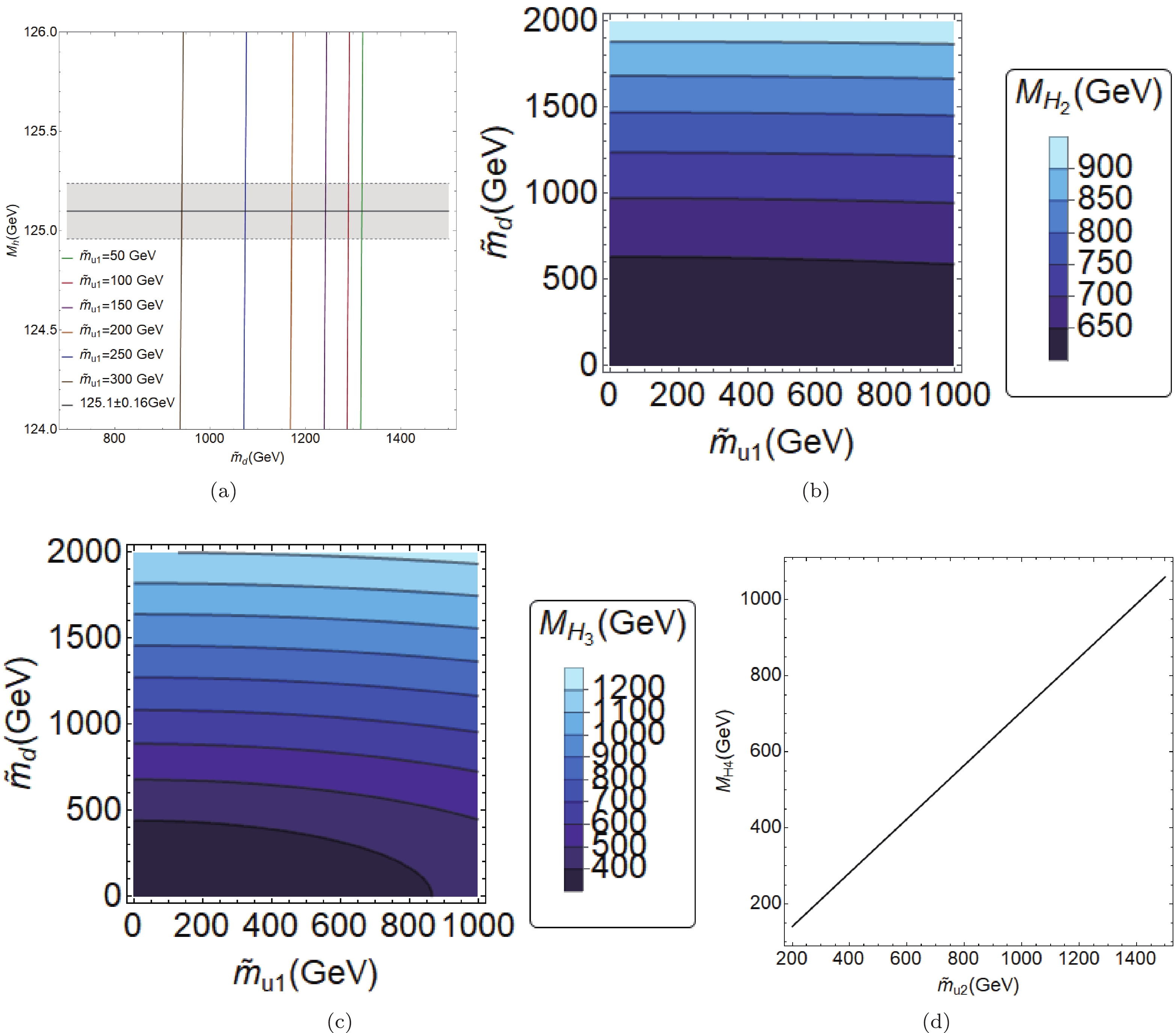 Figure1. (color online) (a) Values of
 Thereafter, in Figs. 1(b)-(c), we present the contour regions for the mass of the heavier scalars
2
A.Yukawa Lagrangian
The Yukawa Lagrangian for this model can be derived from the corresponding superpotential after eliminating the auxiliary fields (F-terms), and it can eventually be written as follows $ \begin{aligned}[b]{\cal{L}} =& \bar{u}_{i{\rm L}}u_{j{\rm R}}(Y^u_1)_{ij}H^0_{u1}+\bar{u}_{i{\rm L}}u_{j{\rm R}}(Y^u_4)_{ij}H^0_{u2}\\&+\bar{d}_{i{\rm L}}d_{j{\rm R}}(Y^d)_{ij}H^0_d+\bar{l}_{i{\rm L}}l_{j{\rm R}}(Y^l)_{ij}H^0_l+{\rm h.c.} \end{aligned} $  | (35) |
$ M_f = Y ^f \frac{v_f}{\sqrt{2}}, $  | (36) |
After rotating to the mass eigenstate basis, both the charged leptons and down type quark Yukawa matrices become diagonal:
$ \bar{Y}^f = \frac{\sqrt{2}}{v_f}\bar{M}_f. $  | (37) |
$ M_u = \frac{1}{\sqrt{2}}\left(v_1 Y^u_1+v_4 Y^u_4\right). $  | (38) |
$ \bar{M}_u = {\cal{V}}_{\rm L} M_u{\cal{V}}^\dagger_{\rm R} = {\cal{V}}_{\rm L} \frac{1}{\sqrt{2}}\left(v_1 Y^u_1+v_4 Y^u_4\right) {\cal{V}}^\dagger_{\rm R}, $  | (39) |
2
B.FCNC Higgs interactions and up-type quark mass matrix with four-texture type
In the use of textures within the context of the 2HDM, a specific form with six zeroes was first considered [24], and it was found that the textures implied a pattern for the Higgs-fermion couplings of the formFor completeness, we include the form of the four-zero texture matrix, namely
$ {M_u} = \left( {\begin{array}{*{20}{c}}0&D&0\\{D*}&C&B\\0&{B*}&A\end{array}} \right). $  | (40) |
The Lagrangian for the up-quarks sector is
$ {\cal{L}}_u = \bar{u}_{i{\rm L}}u_{j{\rm R}}(Y^u_1)_{ij}H^0_{u1}+\bar{u}_{i{\rm L}}u_{j{\rm R}}(Y^u_4)_{ij}H^0_{u2}+{\rm h.c.} $  | (41) |
$ \begin{aligned}[b] {\cal{L}}_u =& \bar{u}_{i{\rm L}}u_{j{\rm R}}(Y^u_1)_{ij}\frac{1}{\sqrt{2}}(v_1+\eta_1+{\rm i}\chi_1)\\&+\bar{u}_{i{\rm L}}u_{j{\rm R}}(Y^u_4)_{ij}\frac{1}{\sqrt{2}}(v_4+\eta_4+{\rm i}\chi_4)+{\rm h.c.}, \end{aligned}$  | (42) |
$ \begin{aligned}[b]{\cal{L}}_u =& \bar{u}_{\rm L}\left[\frac{1}{\sqrt{2}}(v_1Y^u_1+v_4Y^u_4)\right]u_{\rm R}\\&+\bar{u}_{\rm L}\left[\frac{1}{\sqrt{2}}(\eta_1Y^u_1+\eta_4Y^u_4)\right]u_{\rm R}+{\rm h.c.},\\ =& \bar{u}_{\rm L}M_u u_{\rm R}+\bar{u}_{\rm L}\left[\frac{1}{\sqrt{2}}(\eta_1Y^u_1+\eta_4Y^u_4)\right]u_{\rm R}+{\rm h.c.}\end{aligned}$  | (43) |
$ \begin{aligned}[b] \bar{M_u} =& V_{\rm L} M_u V_{\rm R}^\dagger = \frac{v_1}{\sqrt{2}}V_{\rm L}Y^u_1V^\dagger_{\rm R}\\&+\frac{v_2}{\sqrt{2}}V_{\rm L}Y^u_4V^\dagger_{\rm R} \\=& \frac{v_1}{\sqrt{2}}\tilde{Y}^u_1+\frac{v_2}{\sqrt{2}}\tilde{Y}^u_4, \end{aligned}$  | (44) |
$ {\cal{L}}_u = \bar{u}_{\rm L}\bar{M}_u u_{\rm R}+\bar{u}_{\rm L}\left[\frac{1}{\sqrt{2}}(\eta_1\tilde{Y}^u_1+\eta_4\tilde{Y}^u_4)\right]u_{\rm R}+{\rm h.c.} $  | (45) |
$ \tilde{Y}^u_1 = \frac{\sqrt{2}}{v_1}\bar{M}_u-\frac{v_4}{v_1}\tilde{Y}^u_4, $  | (46) |
When rewriting the Lagrangian in terms of
$ \begin{aligned}[b] {\cal{L}}_u =& \bar{u}_{\rm L}\bar{M}_u u_{\rm R}+\frac{1}{\sqrt{2}}\bar{u}_{\rm L}\left[\left(\frac{\sqrt{2}}{v_1}\bar{M}_u-\frac{v_4}{v_1}\tilde{Y}^u_4\right)\eta_1\right.\\&+\tilde{Y}^u_4\eta_4\Bigg]u_{\rm R}+{\rm h.c.} \end{aligned}$  | (47) |
Thus, by using Eq. (26), we obtain the Higgs couplings in the up-type quark sector (with
$ g_{h_1u_iu_j} = \frac{c_\omega c_{\delta _1}c_{\delta _2}}{vc_\beta}\left[\sqrt{2}(\bar{M}_u)_{ij}-vt_\omega s_\alpha c^{-1}_\omega (\tilde{Y}^u_4)_{ij}\right], $  | (48) |
$ \begin{aligned}[b] g_{h_2u_iu_j} =& -\frac{c_\omega(c_{\delta _3 }s_{\delta _1}+c_{\delta _1}s_{\delta _2}s_{\delta _3} )}{vc_\beta}\\&\times\left[\sqrt{2}(\bar{M}_u)_{ij}-vt_\omega s_\alpha c^{-1}_\omega (\tilde{Y}^u_4)_{ij}\right], \end{aligned}$  | (49) |
$\begin{aligned}[b] g_{h_3u_iu_j} =& \frac{c_\omega(s_{\delta _1}s_{\delta _3}-c_{\delta _1}c_{\delta _3} s_{\delta _2} )}{vc_\beta}\\&\times\left[\sqrt{2}(\bar{M}_u)_{ij}-vt_\omega s_\alpha c^{-1}_\omega (\tilde{Y}^u_4)_{ij}\right], \end{aligned} $  | (50) |
$ g_{h_4u_iu_j} = (\tilde{Y}^u_4)_{ij}, $  | (51) |
$ g_{h_1dd} = \frac{\bar{M}_d}{vs_\beta}c_\omega c_{\delta _2}s_{\delta _1}, $  | (52) |
$ g_{h_2dd} = \frac{\bar{M}_d}{vs_\beta}c_\omega(c_{\delta _1}c_{\delta _3}-s_{\delta _1}s_{\delta _2}s_{\delta _3}), $  | (53) |
$ g_{h_3dd} = -\frac{\bar{M}_d}{vs_\beta}c_\omega(c_{\delta _3}s_{\delta _1}s_{\delta _2}+c_{\delta _1}s_{\delta _3}), $  | (54) |
$ g_{h_1ll} = \frac{\bar{M}_l}{vt_\omega c_\alpha}c_\omega s_{\delta _2}, $  | (55) |
$ g_{h_2ll} = \frac{\bar{M}_l}{vt_\omega c_\alpha} c_\omega c_{\delta _2}s_{\delta _3}, $  | (56) |
$ g_{h_3ll} = \frac{\bar{M}_l}{vt_\omega c_\alpha} c_\omega c_{\delta _2}c_{\delta _3}. $  | (57) |
$ g_{h_1WW} = 2\frac{m^2_W}{v}c_\omega[c_\beta c_{\delta _1}c_{\delta _2}+ s_\beta c_{\delta _2}s_{\delta _1}+ t_\omega s_\alpha s_{\delta _2}], $  | (58) |
$\begin{aligned}[b] g_{h_2WW} =& 2\frac{m^2_W}{v}c_\omega[-c_\beta(c_{\delta _3}s_{\delta _1}+c_{\delta _1}s_{\delta _2}s_{\delta _3})\\&+ s_\beta (c_{\delta _1}c_{\delta _3}-s_{\delta _1}s_{\delta _2}s_{\delta _3})+ t_\omega s_\alpha c_{\delta _2}s_{\delta _3}], \end{aligned}$  | (59) |
$ \begin{aligned}[b] g_{h_3WW} =& 2\frac{m^2_W}{v}c_\omega[c_\beta(s_{\delta _1}s_{\delta _3}-c_{\delta _1}c_{\delta _3}s_ {\delta _2}) \\& -s_\beta(c_{\delta _3} s_{\delta _1}s_{\delta _2}+c_{\delta _1}s_{\delta _3}) + t_\omega s_\alpha c_{\delta _2}c_{\delta _3}], \end{aligned}$  | (60) |
$ g_{h_4WW} = 2\frac{m^2_W}{v}c_\omega t_\omega c_\alpha. $  | (61) |
Having determined all of the relevant Higgs couplings, we are ready to work on the Higgs phenomenology. However, prior to this, we find it interesting to comment on the MSSM limit of our model. In fact, this was discussed in Ref. [34], which works in the so-called Higgs-basis, where only two doublets develop VEVs. The authors of this reference discussed in detail the issue of the decoupling limit, and although they confirmed that the model was reduced to the SM, in the limit in which all mass-parameters are very large; that is, with no non-decoupling effects from the extra degrees of freedom, they also identified several "quasi-decoupling" effects, which prevented the model from being reduced to the MSSM in that limit. This is owing to the mixing with the extra Higgs doublets, unless the extra b-terms are set to zero, such that no mixing is allowed. However, when using our parameterization for the VEVs, we can observe that in the limits
● The mixing angles
● Angles that parameterize the VEVs:
● Heavy scalar masses: mainly
● Yukawa matrix elements
Moreover, we need to specify the soft SUSY-breaking terms, but these are essentially fixed by requiring the light Higgs boson mass of 125 GeV and the remaining neutral CP-even Higgs masses to be larger than approximately 0.5 TeV.
To provide a realistic scenario, we use the most up-to-date experimental measurements reported by the ATLAS and CMS collaborations [35, 36]; namely, the signal strengths
$ {\cal{R}}_{X} = \frac{\sigma(pp\to h)\cdot BR(h\to X)}{\sigma(pp\to h^{{\rm{SM}}})\cdot BR(h^{{\rm{SM}}}\to X)}, $  | (62) |
Figure 2 presents the plane
 Figure2. (color online) Allowed region in plane
 | Parameter | Value |
  |   |
  |   |
  |   |
  |   |
Table2.Values for additional parameters used to evaluate
Furthermore, we are required to determine the values of the matrix elements
For the high-energy constraints, we use the direct upper limit on
Figure 3 depicts the allowed regions in the plane
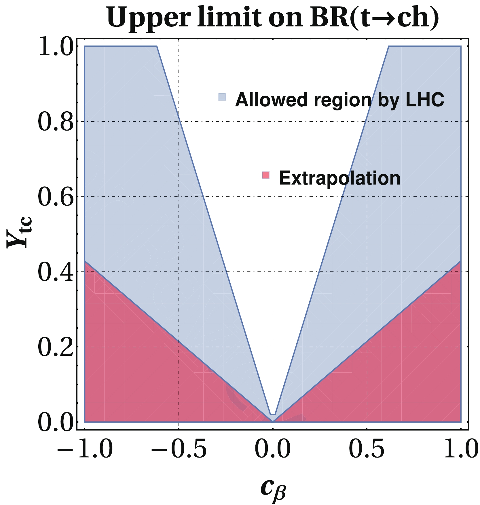 Figure3. (color online) Plane
 Regarding the low-energy constraints, Ref. [40] presented a detailed analysis of the FCNC arising from the 2HDM by incorporating the Cheng-Sher anzast, where the couplings of the Higgs bosons (
Regarding the tree-level neutral Higgs contribution to
Thus, our model parameters satisfy all low-energy constraints, and in fact, the strongest constraints will result from the LHC studies. Table 2 summarizes the benchmark point for the parameters of our model to be used in the subsequent calculations. Furthermore, we set
In the following subsection, we present a detailed study of the detection of the decay
2
A.Search for decay $ {t\to c h} $![]()
![]()
at LHC
The branching ratio for the decay $ {BR}(t\rightarrow c h) = \frac{\Gamma(t\rightarrow ch)}{\Gamma_{\rm tot}}, $  | (63) |
$\begin{aligned}[b] \Gamma(t\rightarrow ch) =& \frac{m_t}{16\pi}g_{htc}^2\left[(1+r_{tc})^2-r_{ht}^2\right] \\&\times\sqrt{1-(r_{ht}+r_{tc})^2}\sqrt{1-(r_{ht}-r_{tc})^2}, \end{aligned} $  | (64) |
In Fig. 4, we display
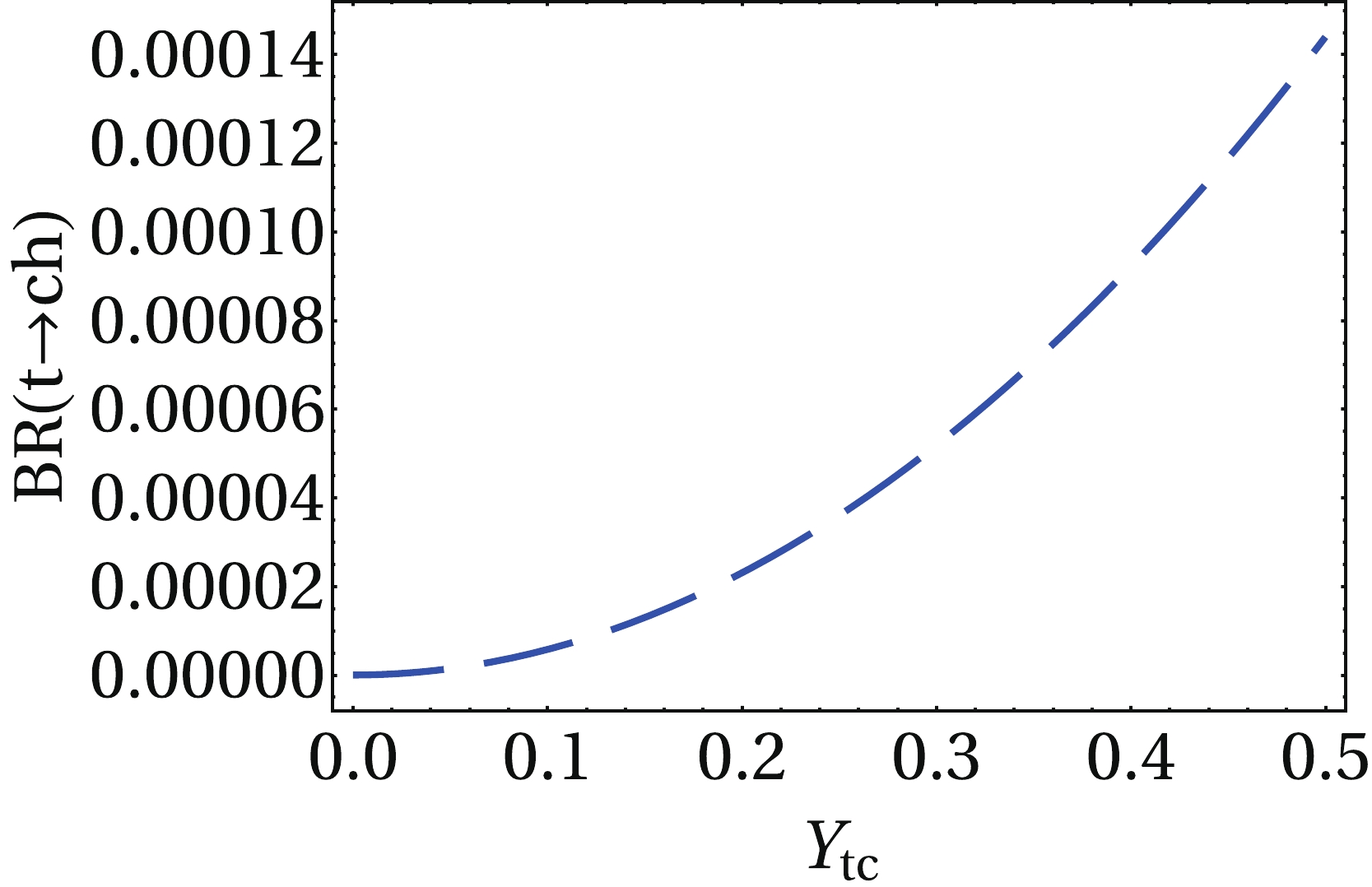 Figure4. (color online) Branching ratio of decay
 The analysis is carried out for the LHC and its next stage; that is, the HL-LHC [50]. We first discuss both the signal and main SM backgrounds for the decay channels of the Higgs boson to be considered. We adopt the strategy carried out by the ATLAS and CMS collaborations [51, 52].
● Signal
We consider top pair production, and subsequently, one top is decayed via the FCNC mode, whereas the other one is decayed through the SM mode. Thus, the signature is
● Background
1. In the case of the diphoton-channel, we study the backgrounds resulting from:
–
–
–
–
2. For the mode
–
–
–
–
However, regarding our computation scheme, we first implement the Feynman rules of the model via
We now turn to evaluate the number of signal events produced as a function of
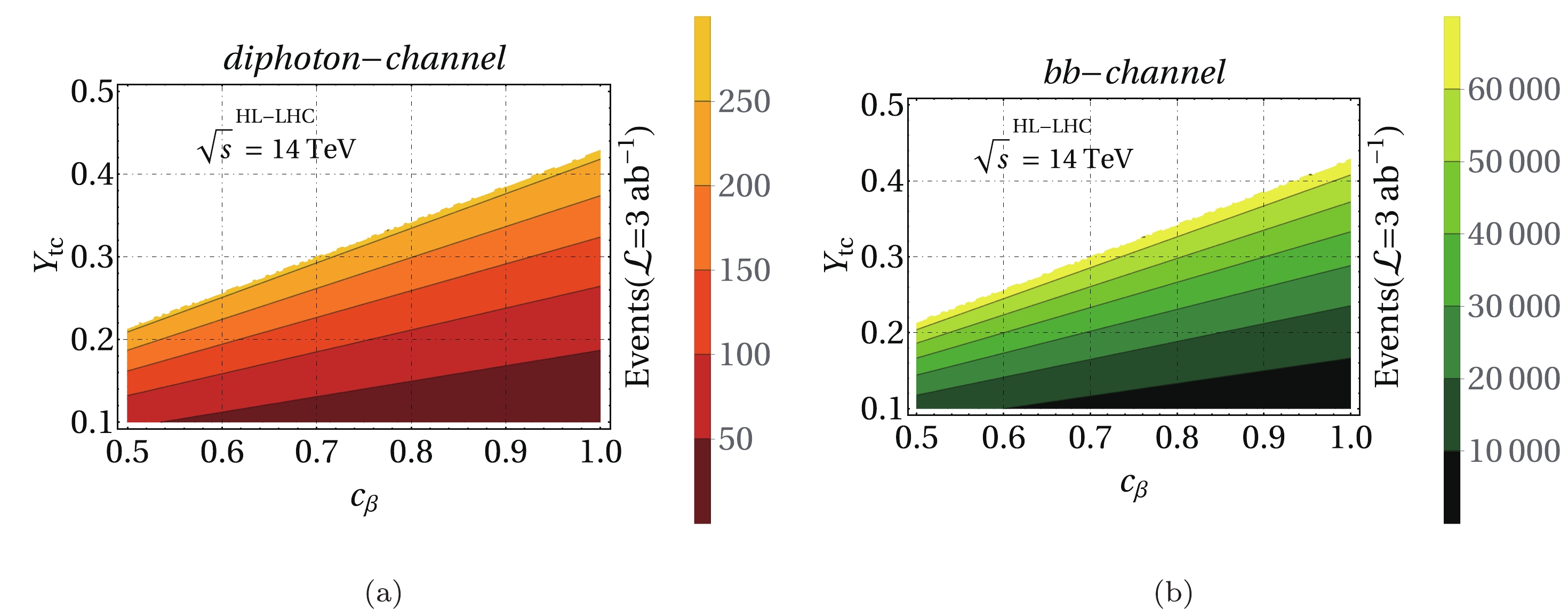 Figure5. (color online) Number of signal events as function of
 The ATLAS and CMS collaborations [51, 52] searched for the decay
● diphoton-channel
1. We require exactly one
2. We identify the charged leptons and photons emerging from the signal imposing
3. The main variable for searching the Higgs boson decay into the diphoton system is the invariant mass
4. Owing to the Higgs boson decays into the diphoton system, it is required that the invariant mass associated with the top quark falls between
5. The separations between the photons resulting from Higgs boson decay must be
6. The separation between the diphoton system and jet is
7. Owing to the non-detected neutrino in the final state, we demand a missing transverse energy
8. The tagging and mistagging efficiencies selected are as follows:
–
–
–
● bb-channel
1. We require exactly four jets: three of them are tagged as
2. Exactly one isolated lepton with
3. To obtain a neutrino that emerges in the final state, the missing transverse energy
4. To reconstruct the top quark mass associated with the FCNC, it is required that
5. Regarding the reconstruction of the Higgs boson mass, it is imposed that
6. It is required that
7. The tagging and mistagging efficiencies selected are as follows:
–
–
–
Subsequently, we evaluate the signal significance
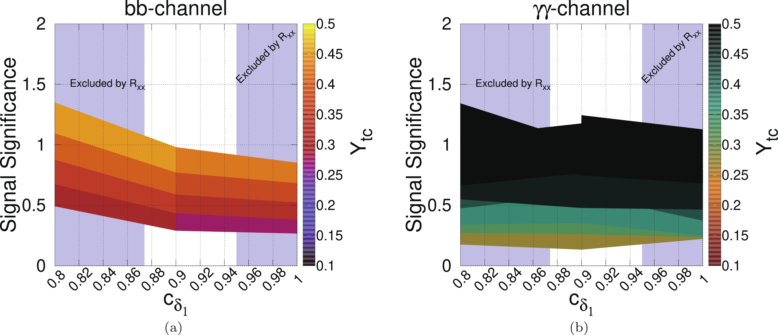 Figure6. (color online) Signal significance as function of
 We can appreciate that for both channels, the values of the significance are of the order 1 for
2
B.Search for decay $ H_2\to tc $![]()
![]()
at LHC
First, we evaluate the relevant decay modes of 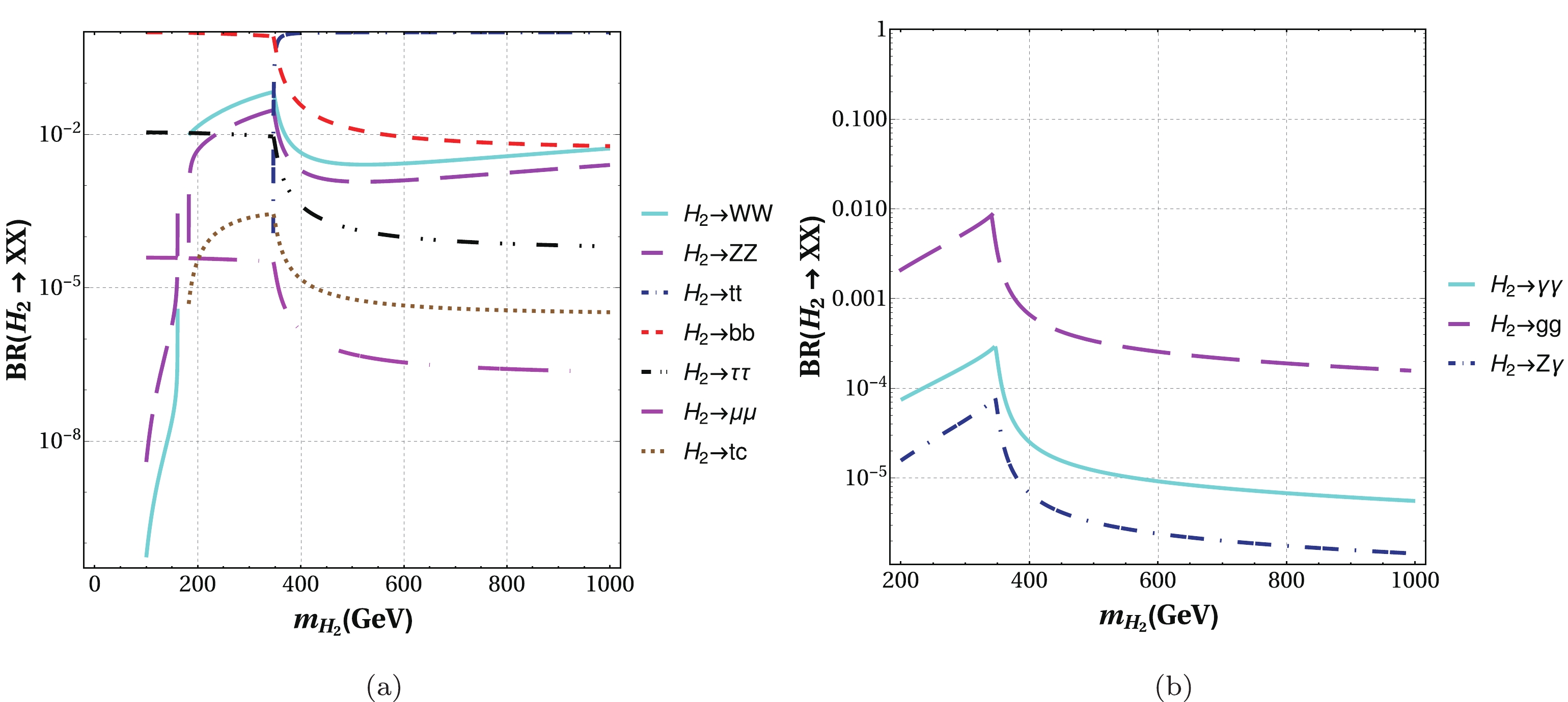 Figure7. (color online) Branching ratio of decays
 We observe that the FCNC mode
For the production of the heavy Higgs boson, we focus on the gluon fusion mechanism, which is the dominant production mechanism for the SM case. The corresponding cross-section is displayed in Fig. 8(a), whereas the number of signal events, considering the optimal integrated luminosity (
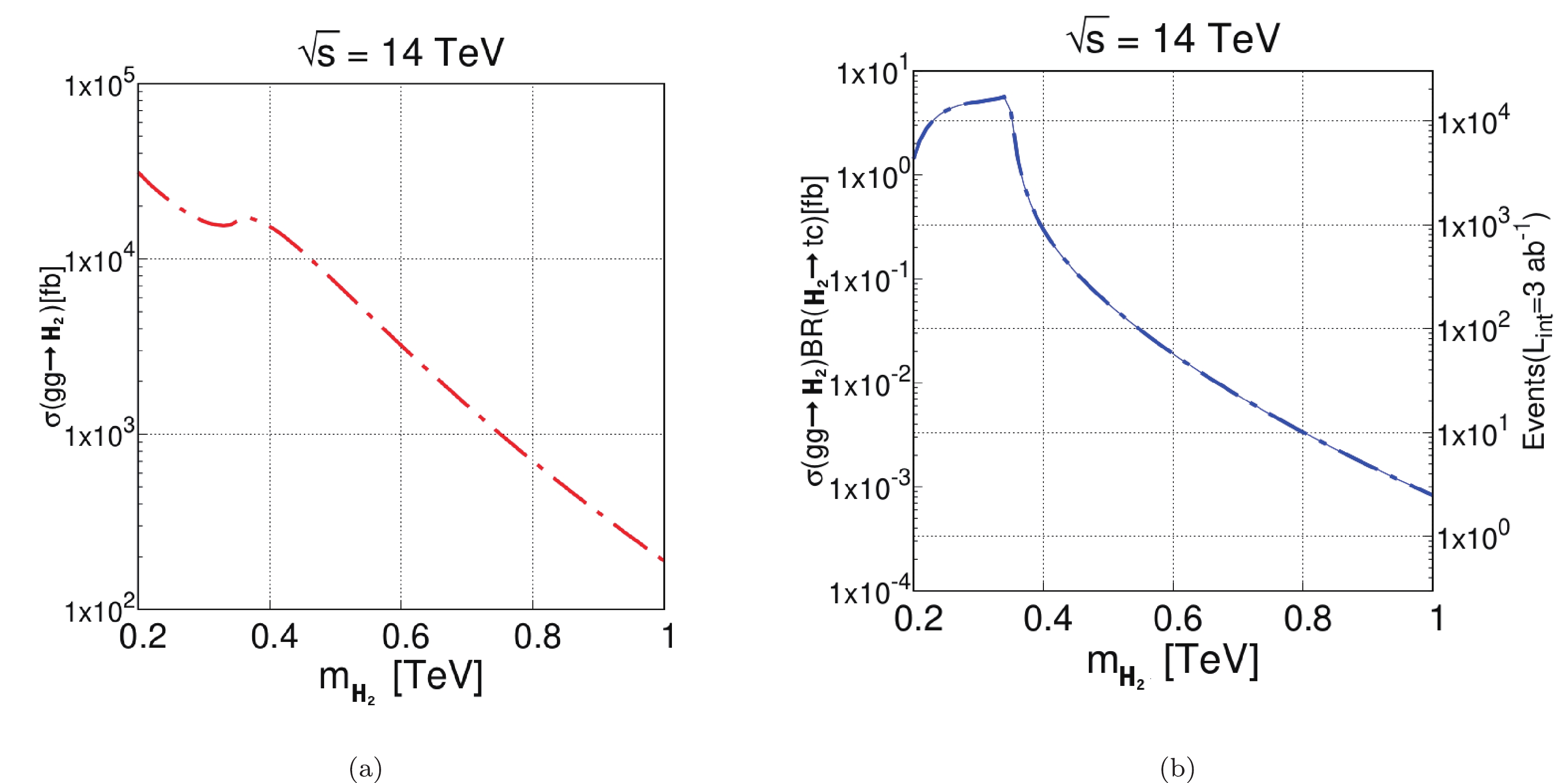 Figure8. (color online) (a)
 As in the previous section, we first define both the signal and the main SM background processes, as follows:
● Signal:
The signature searched is
● Background:
The dominant SM background processes to the final state
1.
2. s and t channel single top
3. Another important background is the
The kinematic cuts imposed are as follows:
● The main kinematic cut to isolate the signal is the transverse mass
$ M_{\rm T}^{\ell} = \sqrt{2|\vec{P}_{\rm T}^{\ell}||\vec{E}_{\rm T}^{\rm{miss}}|(1-\cos\Delta\phi_{\vec{P}_{\rm T}^{\ell}-\vec{E}_{\rm T}^{\rm{miss}}})}. $  | (65) |
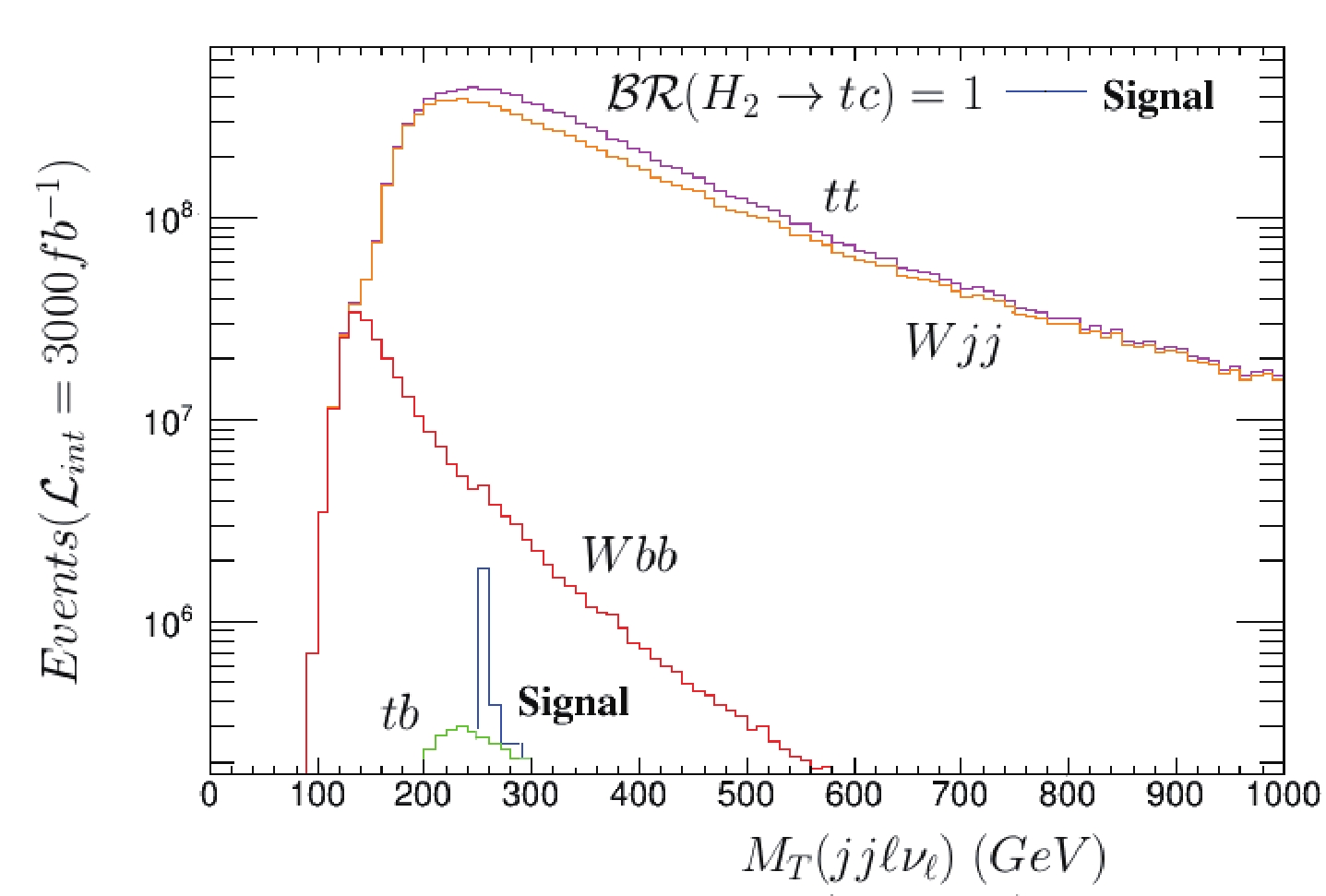 Figure9. (color online) Transverse mass distribution without cuts.
● We require two jets with
● We require one isolated lepton (
● We also consider a cut for the missing transverse energy
After applying the above kinematic cuts (and also considering tagging and mistagging efficiencies as in the previous section) to the signal and main background processes, we can compute the signal significance, which is defined as
Meanwhile, in Fig. 10, we present the contours of the signal significance as a function of the Higgs boson mass
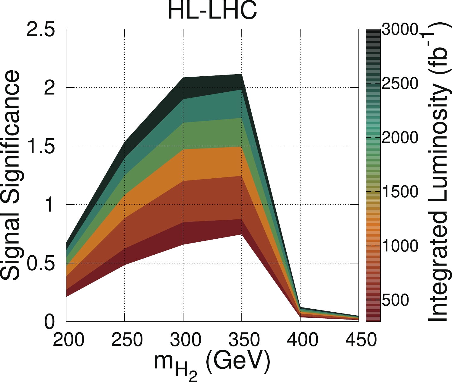 Figure10. (color online) Signal significance as function of integrated luminosity and
 From Fig. 10 that the largest significance can be achieved with the largest luminosity for a certain range of Higgs masses. For example, it will be possible to achieve a significance of 2.1
For the allowed region of the parameter space, we calculated the branching ratio for the decay
We also studied the FCNC decay of the next-to-lightest neutral CP-even Higgs boson,
