Su-Ya Bie ^1,
, Guo-Li Liu ^1,,
, Wenyu Wang ^2,,
,

Corresponding author: Guo-Li Liu, guoliliu@zzu.edu.cn

Corresponding author: Wenyu Wang, wywang@bjut.edu.cn

1.School of Physics and Microelectronics, Zhengzhou University, Zhengzhou 450001, China
2.School of Physics, Beijing University of Technology, Beijing 100124, China
Received Date:2020-06-23
Available Online:2021-01-15
Abstract:The decay $t \to c V $ ($V=\gamma,~Z,~g$) processes in mirror twin Higgs models with colorless top partners are studied in this paper. We report that the branching ratios of these decays can strongly affect the standard model expectations in some parameter spaces and may be detectable according to the current precision electroweak measurements. Thus, constraints on the model parameters may be obtained from the branching fraction of the decay processes, which may serve as a robust detection tool for this new physics model.

HTML

--> --> -->

In contemporary high energy physics, one of the most important questions is whether the Higgs mass tuning indeed exists in nature, or whether the electroweak scale is set by a mechanism that does not need a large cancellation. This is the issue of the Higgs naturalness, or the hierarchy problem.
An attractive dynamical model for solving the hierarchy problem introduces a new symmetry, which protects the Higgs particle against large radiative corrections. That is, these models invoke such a symmetry that implies the existence of particles beyond the standard model (SM), which consists of the "symmetry partners" of known SM fields.
The hierarchy problem depends on the top quark one loop diagram; therefore, ANY model that resolves the hierarchy problem must introduce top quark symmetry partners, i.e., the so-called "top partners." In contrast, to avoid significant residual tuning, these top partners are expected to have masses at or below the TeV scale. For example, in supersymmetric models (for a review, see [1]) and in little Higgs models [2-5] (for a review, see [6]), there exist scalar stops and vector-like fermionic top-primes as top partners, respectively. In these models, the new symmetry protects the Higgs from commuting with the SM gauge symmetries; thus, the quantum numbers of the top partners are identical to those of the top quark.
The search for these colored top partners, both scalar and fermionic, however, had so far suffered stringent limits associated with the large hadron collider (LHC) searches (e.g., [7-10]); thus, theories that include colorless top partners, i.e., not charged under strong interactions, are increasingly compelling. Since the production cross sections of uncolored top partners are many orders of magnitude smaller than those of the colored case, a simple understanding can be developed for explaining why these particles have so far escaped discovery.
Colorless top partners occur in scenarios where the symmetry is localized rather than global (as in little Higgs theories) [11-13]. By far, the most striking possibility of uncolored top partners is the mirror twin Higgs (MTH) model, where the Higgs is protected by the discrete $ Z_2 $ subgroup [11] (see also [13-17]).
In contrast, the huge mass of the top quark significantly shortens its lifetime, and it decays without non-perturbative hadronization effects. Thus, there is still some room for non-standard top quark interactions, such as productions and decays. Moreover, the top quark strongly interacts with the yet-mysterious Higgs boson. Thus, detailed studies of top-quark interactions would be useful for exploring the mechanism of the electroweak symmetry breaking, as well as some properties of the Higgs boson.
In the SM, flavor changing neutral currents (FCNCs) are absent from the tree-level, while on the loop-level, they are strongly suppressed by the Glashow-Iliopoulos-Maiani (GIM) mechanism. Within the SM, the decays of the top quark induced by the FCNC interactions are known to be extremely rare. Thus, the FCNC interactions are of utmost importance in constraining the beyond SM (BSM) physics. However, these loop-driven processes can get contributions from new physics particles and new couplings and can significantly alter the SM predictions for these processes. In the present paper, we consider the rare decays of $ t\to cV $ ($ V = \gamma,\; Z,\; g $) in the context of MTH models.
The remainder of this paper is organized as follows. In Sec. II, we briefly describe the realization of the considered MTH models with colorless top partners and introduce related couplings with the top rare decay. Section III is dedicated to discussions about the calculation of the three decay processes in these models. The results are elaborated in Sec. IV. Section V summarizes the compatibility of parameter spaces with phenomenological constraints coming from the electroweak precision data (LHC observations). Finally, a summary and conclusions are given in Sec. VI.

2

-->

A.The model and cancellation mechanism

The MTH models assume a $ Z_2 $ distinct symmetry that exchanges the complete SM with a mirror copy of the SM; this copy is called the twin sector. In addition, the global symmetry of the Higgs sector of the theory is approximate, which may be taken as either SU(4)$ \times $U(1) or O(8) and the SM Yukawa couplings, and the SM electroweak gauge interactions explicitly violate global symmetry. The gauge subgroup contains the SU(2)$ \times $U(1) electroweak interactions of the SM and of the twin sector. After the global symmetry is spontaneously broken, the SM Higgs doublet emerges as a light pseudo-Nambu-Goldstone boson. Although the global symmetry is violated, the discrete $ Z_2 $ symmetry, however, is exact, ensuring the absence of quadratically divergent contributions to the Higgs mass on the one-loop level.
In the following, the SU(4)$ \times $U(1) group is taken as an example global symmetry, to describe the cancellation of the quadratic divergences in this model, and the gauge subgroup of the SM and twin sectors can be taken as SU(2)$ \times $SU(2)$ \times $U(1) and $ U(1) $, respectively. Labels A and B will be used to denote the SM and twin sectors, and under the action of the discrete $ Z_2 $ symmetry, the labels A and B become exchangeable, i.e., $ A \leftrightarrow B $. Then, the field H, which transforms as the fundamental representation under the global SU(4) symmetry, can be written as

$ H = \left(\begin{array}{c} H_A\\ H_B \end{array} \right) \; , $

(1)

where $ H_A $ and $ H_B $ represent the SM Higgs doublet and the twin doublet, respectively.
The SU(4) potential for H is

$ m^2 H^{\dagger}H + \lambda (H^{\dagger} H)^2 .$

(2)

When the parameter $ m^2 $ is negative, the global symmetry is spontaneously broken, SU(4)$ \times $U(1)$ \to $ SU(3)$ \times $U(1), and thus, the gauge and Yukawa interactions engender radiative corrections that violate the global symmetry and generate a mass for $ H_A $.
To cancel the quadratically divergent corrections, the top Yukawa coupling can be taken as

$ \lambda_{Ai} H_A q_{Ai} t_A + \lambda_{Bi} H_B q_{Bi} t_B \,. $

(3)

Owing to the $ Z_2 $ symmetry, $ \lambda_{At} = \lambda_{Bt} = \lambda $, so that, on the one loop level, quadratically divergent corrections to the Higgs potential can be generated and canceled out by these interactions. The corrections are as follows ($ \Lambda $ is the ultraviolet (UV) cutoff):

$ \Delta V = \frac{3}{8 \pi^2} \Lambda^2 \left(\lambda_{At}^2 H_A^{\dagger} H_A + \lambda_{Bt}^2 H_B^{\dagger} H_B \right) = \frac{3 \lambda^2}{8 \pi^2} \Lambda^2 H^{\dagger} H \;\; . $

(4)

Thus, with the $ Z_2 $ symmetry, the above contribution conforms to the global symmetry; thus, it cannot contribute to the mass of the Nambu-Goldstone bosons.
More generally, the cancellation mechanism of the Higgs mass can also be understood in the framework of the low effective theory. H can then be written as

$ H = \left(\begin{array}{c} H_A\\ H_B \end{array} \right) = \exp\left(\frac{i}{f}\Pi \right)\left(\begin{array}{c} 0\\ 0\\ 0\\ f \end{array} \right) \; . $

(5)

Where f is the symmetry breaking vacuum expectation value (VEV), and $ \Pi $ is

$ \Pi = \left(\begin{array}{ccc|c} 0&0&0&h_1\\ 0&0&0&h_2\\ 0&0&0&0\\ \hline h_1^{\ast}&h_2^{\ast}&0&0 \end{array} \right). $

(6)

Expanding the exponential, we have

$ H = \left(\begin{array}{c} {{h}}d\dfrac{if}{\sqrt{{{h}}^{\dagger}{{h}}}}\sin\left(\dfrac{\sqrt{{{h}}^{\dagger}{{h}}}}{f} \right)\\ 0\\ f\cos\left(\dfrac{\sqrt{{{h}}^{\dagger}{{h}}}}{f} \right) \end{array} \right), $

(7)

where $ {{h}} = (h_1, h_2)^{\rm{T}} $ is the Higgs doublet of the SM

$ H_A = {{h}}\frac{if}{\sqrt{{{h}}^{\dagger}{{h}}}}\sin\left(\frac{\sqrt{{{h}}^{\dagger}{{h}}}}{f} \right) = i {{h}}+\ldots\,, $

(8)

$ H_B = \left(\begin{array}{c} 0\\ f\cos\left(\dfrac{\sqrt{{{h}}^{\dagger}{{h}}}}{f} \right) \end{array} \right) = \left(\begin{array}{c} 0\\ f-\dfrac{1}{2f}{{h}}^{\dagger}{{h}}+\ldots \end{array} \right). $

(9)

Now, considering Eq. (3) in the quadratic order of $ {{h}} $,

$ i\lambda_i{{h}} q_{Ai}t_A+\lambda_i\left(f-\frac{1}{2f}{{h}}^{\dagger}{{h}} \right) q_{Bi}t_B \; . $

(10)

Thus, the quadratic divergence arising from the first diagram is exactly canceled by that of the second via evaluating these contributions.
2 -->

B.The quark flavor changing couplings

Now, we focus on the flavor changing of the top quark. Firstly, we determine the low energy couplings of the Higgs. Choosing the unitary gauge in the visible sector, with $ h_1 = 0 $ and $ h_2 = (v+\rho)/\sqrt{2} $, we obtain

$ \begin{array}{cc} H_A = \left(\begin{array}{c} 0\\ if\sin\left(\dfrac{v+\rho}{\sqrt{2}f} \right) \end{array}\right), &H_B = \left(\begin{array}{c} 0\\ f\cos\left(\dfrac{v+\rho}{\sqrt{2}f} \right) \end{array}\right). \end{array} $

(11)

The kinetic terms are

$ \left|D_{\mu}^AH_A \right|^2+\left|D_{\mu}^BH_B \right|^2 , $

(12)

where $ D^{A,B} $ denotes the covariant derivative of the $ A,B $ gauge bosons. From the above equation, one can obtain the masses of the $ W^\pm $ and Z gauge bosons in the visible sector A and twin sectors B and their couplings to the Higgs, $ \rho $, which determine the relation of the Higgs SM VEV $ v_{\rm{EW}} = $246 GeV and the MTH parameters v and f,

$ v_{\rm{EW}} = \sqrt{2}f\sin\left(\frac{v}{\sqrt{2}f} \right)\equiv\sqrt{2}f\sin\vartheta \; , $

(13)

where the angle $ \vartheta = \dfrac{v}{\sqrt{2}f} $, and when $ v = v_{\rm{EW}} $, $ v \ll f $, or equivalently, $ \vartheta\ll 1 $.
Expanding the top quark sector (3) in the unitary gauge,

$ \begin{aligned}[b] &\lambda_i\left[ifq_{Ai}t_A\sin\left(\frac{v+\rho}{\sqrt{2}f} \right) +fq_{Bi}t_B\cos\left(\frac{v+\rho}{\sqrt{2}f}\right) \right]\\ = &i\frac{\lambda_i v_{\rm{EW}}} {\sqrt{2}}q_{Ai}t_A\left[1+\frac{\rho}{v_{\rm{EW}}}\cos\vartheta \right]\\&+ \lambda_i fq_{Bi}t_B\cos\vartheta \left[ 1-\frac{\rho}{v_{\rm{EW}}} \tan\vartheta\sin\vartheta \right]. \end{aligned} $

(14)

Here, $ q_i $ can be quarks $ u,\; c $, or t.
From this, we can also see that the mass of the top quark's mirror twin partner is

$ m_T = \lambda_t f\cos\vartheta = m_t\cot\vartheta\, . $

(15)

From Eq. (14), we can also see clearly that the scalar $ \rho $ acts as the SM-like Higgs, and it consists of both visible and invisible parts in some ratio, according to certain parameters.

From Eq. (14), we can see the flavor changing couplings mediated by the neutral scalar, so the FCNC decays $ t\to c V $ can be realized by it, and the Feynman diagrams are listed in Fig. 1. We can see from Eq. (14) that the structure of the fermions' couplings to the scalar $ \rho $ is very simple. To be more general, we write the couplings of the scalar to the fermions as
Figure1. (color online) Feynman diagrams for the process $ t\to cV $ in the 't Hooft–Feynman gauge in the MTH model.

$ \rho q_{Ai}\bar t_A: i\frac{\lambda_i} {\sqrt{2}} (c+d\gamma^5), $

(16)

where $ q_{Ai} = t,\; c $ (we only consider the visible section A), $ \lambda_c = V_{tc}\lambda_t $, and $ V_{tc} $ is the ratio of the two couplings, somewhat like the CKM matrix element $ U_{tc} $. The parameters c and d expand the Lorentz structure, and from Eq. (14), we see that $c = {1}/{2},\; d = 0$. In the following discussion, however, we also release the constraints and check the influence on the branching ratios in Fig. 3.
2

-->

A.The amplitude and the width of $ t\to cg $, $ t\to c \gamma $, and $ t\to cZ $

With the general coupling of the Yukawa form, we can write out the amplitude of the decay $ t\to cg $(taking Fig. 1 (c) as an example),

$ \begin{aligned}[b] {\cal M}_c=& \bar u_c \left(i\frac{\lambda_c } {\sqrt{2}} \right)(c+d\gamma^5)\frac{i}{{\not\!\! k}-m_t}(-ig_s\gamma^\mu T^a) \frac{i}{{\not\!\! k}+{{\not\!\! p}_g}-m_t} \\&\times\left(-i\frac{\lambda_t } {\sqrt{2}} \right) (c-d\gamma^5) \frac{i}{(k+p_g-p_t)^2-m^2_\rho} u_t \epsilon_\mu \\ = &-\frac{\lambda_c\lambda_t }{2}g_sT^a\frac{1}{k^2-m_t^2}\frac{1}{(k+p_g)^2-m_t^2}\frac{1}{(k+p_g-p_t)^2-m^2_\rho} \\&\times \bar u_c (c+d\gamma^5)({\not \!\!k}+m_t)\gamma^\mu({\not\!\! k}+{{\not\!\! p}_g}+m_t)(c-d\gamma^5)u_t \epsilon_\mu \,.\end{aligned} $

Note that in the above formula, we have omitted the common integrated factor $\tau^{2\epsilon }\displaystyle\int^{+\infty}_{-\infty} \dfrac{{\rm d}^nk}{(2\pi)^n}$, where $ \epsilon = 1-\frac{n}{2} $, and$ \tau $ is the scale factor introduced for keeping the dimensionality of the coupling constants unchanged. The decay width in general is given by

$ \Gamma_{t\to cg} = C_F \frac{1}{32\pi}|M|^2 , $

(17)

where $ C_{F} = 4/3 $ is a color factor.
As for the width of $ t\to c\gamma $, we can simply obtain it by replacing the coupling $ g_s $ with e in the amplitude and $ C_{F} $ with $ 1 $. Since the coupling of $ Z\bar t t $ is slightly more complicated than that of $ \gamma \bar t t $, in the calculation of $ t\to c Z $, we need to replace the $ t\to c\gamma $ parameters e with $ e/(2s_Wc_W) $ and the structure $ \gamma^\mu $ with $ \gamma^\mu(P_L-2s_W^2) $.
In this scalar-mediated decay process, one-loop divergent terms add up to zero. In other words, one-loop divergences mutually cancel out in the Feynman gauge, so we can safely use the calculating tool of LoopTools [19].
Of course, the effective vertex $ \bar{t}cV $ is a 4-component Lorentz vector and a $ 4 \times 4 $ matrix in the Dirac space and needs to be managed. Note that the tensor loop functions can be retained rather than expanding them in terms of the scalar loop functions as usual [20].
In the Fortran realization, a three-dimensional array $ V(i,j,k) $ with i (= 1,2,3,4) labeling the Lorentz indices and $ j,k $ (= 1,2,3,4) labeling the spinor indices is used. More details are provided in Ref. [21].
2 -->

B.Top total width and upper bounds on rare decays

The decay width of the dominant decay mode of the top quark $ t\to bW $ is given by [22, 23]

$ \begin{align} \Gamma_{t\to bW} = \frac{G_{F}}{8\sqrt{2}\pi}|V_{tb}|^{2} m_{t}^{3} \left[ 1 - 3\left(\frac{m_{W}}{m_{t}}\right)^{4} + 2\left(\frac{m_{W}}{m_{t}}\right)^{6} \right]. \end{align} $

(18)

The above equation gives $ \Gamma_{t\to bW} \sim 1.5 $ GeV. Thus, the branching ratio of any other mode $ t\to X $ is

$ {\rm{BR}}(t\to X) = \frac{\Gamma_{t\to X}}{\Gamma_{t\to bW}}. $

(19)

The SM predictions for the $ t\to cg $, $ t \to c\gamma $ and $ t\to cZ $ branching ratios are [22-25]

$ {\rm{BR}}(t\to cg) = \left(4.6^{+1.1}_{-0.9} \pm 0.4^{+2.1}_{-0.7} \right)\times 10^{-12}, $

(20)

$ BR(t \to c\gamma) = \left(4.6^{+1.2}_{-1.0}\pm 0.4^{+1.6}_{-0.5} \right)\times 10^{-14}, $

(21)

$ {\rm{BR}}(t\to cZ) = (1.03\pm 0.06)\times 10^{-14}, $

(22)

The LHC has searched for these rare decays and yielded their upper bounds [26-31]:

$ {\rm BR}(t\to cg) < 2\times 10^{-4}. $

(23)

$ {\rm BR}(t\to cZ) < 2\times 10^{-4}. $

(24)

$ {\rm BR}(t \to c\gamma)< 1.82\times 10^{-3}. $

(25)

From Eq. (23) to Eq. (25), we see that the predictions of the SM, Eq. (20) to Eq. (22), cannot be probed at the LHC, so any signal of the flavor decays of this kind inevitably indicates new physics.
Some BSM scenarios may predict an enhanced branching ratio of these rare modes up to the level that can be detected in future colliders, such as 2HDM [24, 32, 33], left-right symmetric model [34], MSSM [21], R-parity violating SUSY [35], warped extra dimensional models [36, 37], UED models [38], mUED and nmUED models [22, 23], and composite Higgs model [39, 40]. In Refs. [41, 42], the effective Lagrangian approach is used for studying rare top decays. Other collider studies on the search of these rare decays can be found in Refs. [43-55]. In what follows, we check whether the predictions of the MTH models are detectable, and we provide some constraints on the model parameters.
2 -->

C.The results for $ t\to cV $

To determine constraints on the parameter f, the VEV v (determine the relation between it and the electroweak VEV 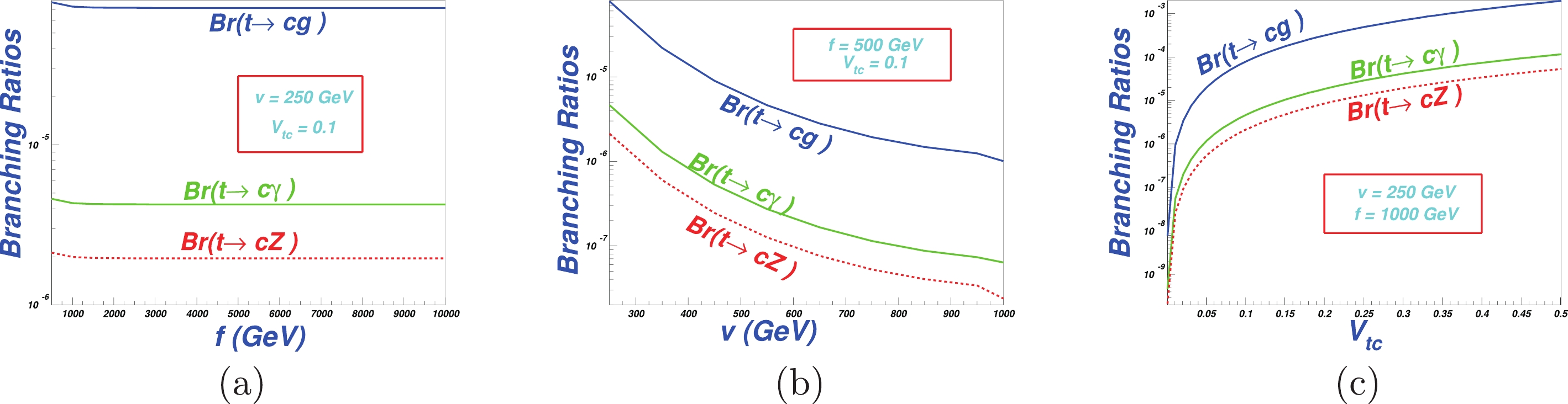$v_{\rm EW}$; one can refer to Eq. (13)), and the flavor changing coupling $ V_{tc} $, the one-loop level branching ratios of the three processes are shown in Fig. 2. We set $ m_t = 172.5 $ GeV and $ M_Z = 91.2 $ GeV, and other physical constants are obtained from Ref. [56].
Figure2. (color online) One-loop level branching ratios of the three processes in the MTH model.

The plots in Fig. 2 show that the branching ratios are in the following respective ranges: ${\rm BR}(t\to cg) \sim 10^{-3}-10^{-6}$, ${\rm BR}(t\to c\gamma) \sim 10^{-4}-10^{-8}$, and ${\rm BR}(t\to cZ) \sim 10^{-5}-10^{-8}$. The reason that $ t\to cg $ is larger than $ t\to c\gamma\; /Z $ is that the $ g\bar q q $ coupling in this process with QCD coupling $ \alpha_S $ involved is one order larger than the electroweak coupling $ \gamma \bar q q \sim \alpha_e $.
We see from Fig. 2 that the influences of the parameters on the branching ratios are not the same: varying f or v does not make much difference when the other parameters are fixed, as shown in Fig. 2(a)(b), while varying $ V_{tc} $ significantly changes the branching ratios. However, the alteration is an associative effect of the parameters f, v, and $ V_{tc} $, since in the couplings in Eq. (16), $ \lambda_c $ is connected with all three and therefore does not quadratically increase with increasing $ V_{tc} $.
From Fig. 2, we also see that the process $ t\to cg $ promises to be detectable, according to the experimental bounds in Eqs. (23), (24), (25), and may provide constraints on the parameters. Thus, in the following, we only consider the process $ t\to cg $.
To reveal the effect of the structural parameters c and d in Eq. (16) on the branching ratio of $ t\to cg $, in Fig. 3, we vary c between $(-{1}/{2},{1}/{2})$ with $d = 0,\; c,\; {1}/{2}$, respectively. We find that c and d cannot be equal to zero simultaneously, because if this happens, the coupling $ \rho \bar q_i t $ will vanish, and so will the $ t\to cg $ branching ratio. Normally, these values should be $\pm{1}/{2}$ and $ 0 $ (asynchronously).
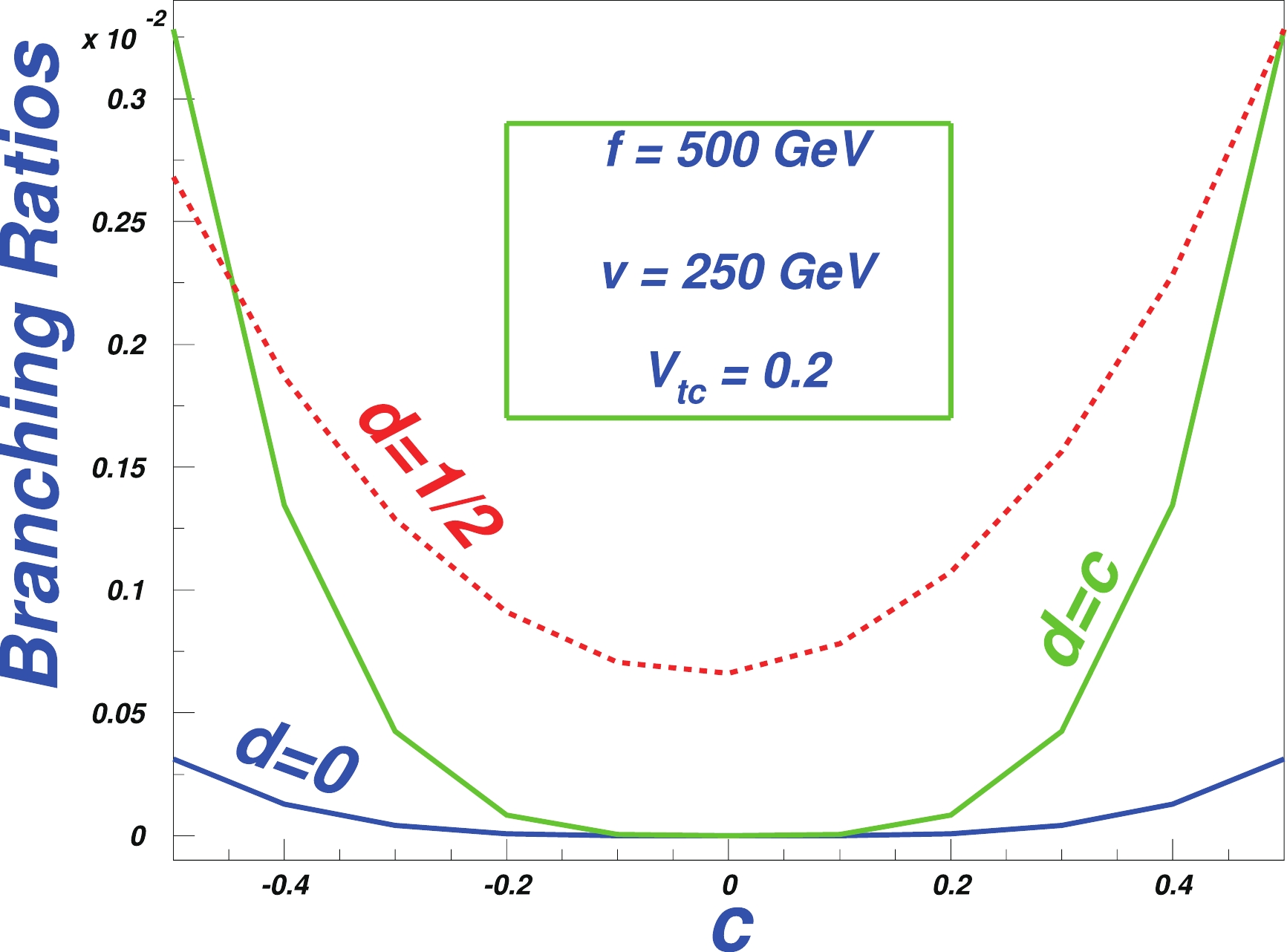Figure3. (color online) One-loop level branching ratios of the three processes in the MTH model versus the structure parameter c.

In Figs. 2 and 3, the parameter values are in the optimal range: we set $ v = 250 $ GeV, $ f = 500 $ GeV, and $ V_{tc} = 0.2 $, i.e., quite a strong coupling. However, actually, the values of these parameters may not be optimized for detection by colliders; thus, we scanned the entire parametric space, to determine the appropriate range. If signal detection is problematic, the model parameters will be severely constrained. That is, if we cannot find the process, it may serve as a robust measurement for constraining the model parameters, especially $ V_{tc} $.
Figure 4 considers the possibility of the $ t\to cg $ branching ratios in light of detectability, for the following three parameter ranges: $ 500 \leqslant f \leqslant 10000 $ GeV, $ 250 \leqslant v \leqslant 1000 $ GeV, and $ 0.001 \leqslant V_{tc}\leqslant 0.5 $. From Fig. 4(a), we see that the branching ratios prefer small v values, while they are insensitive to f, which is because, from Eq. (13), $\lambda_t = \sqrt{2}m_t/(f \sin\vartheta) = \dfrac{\sqrt{2}m_t}{f \sin [v/(\sqrt{2}f)]}$; thus, the smaller v is, the larger the branching ratio is. In the meantime, with two compelling fs in the denominator, we conclude that v contributes more than f, which is also seen clearly in the next two figures.
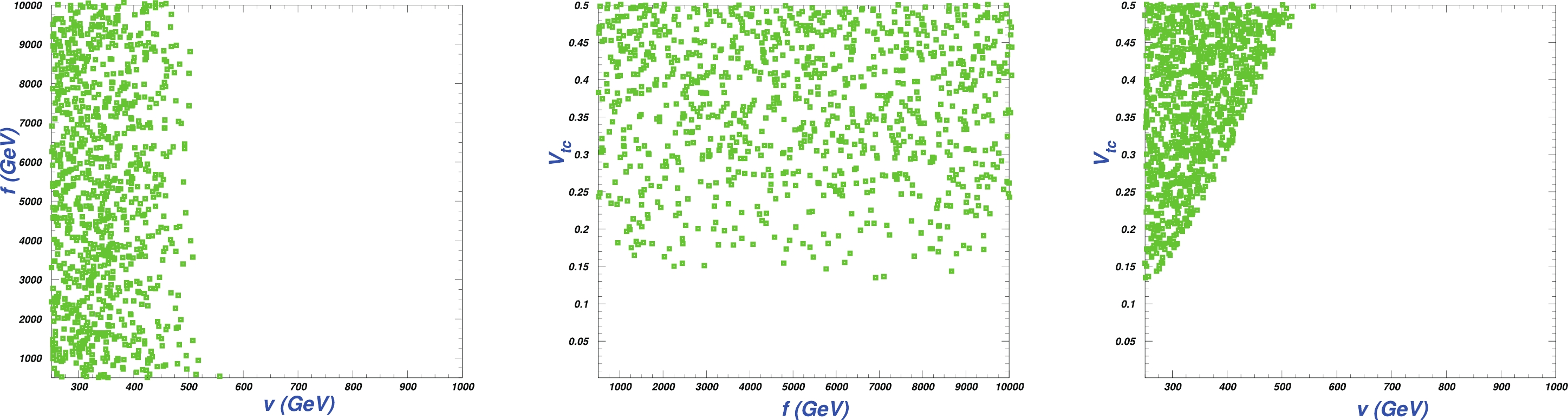Figure4. (color online) The $ t\to cg $ detective contours on $ v\sim f $, $ f\sim V_{tc} $, and $ v\sim V_{tc} $ in the MTH model.

However, $ V_{tc} $ is close to linear in the amplitude, so the branching ratios increase rapidly with increasing $ V_{tc} $. Hence, to arrive at the detectable level, larger $ V_{tc} $ values are preferable, which can be seen clearly in Fig. 4(b)(c).
From Fig. 4, we see that the parameters are constrained in a very narrow space, if the FCNC decay $ t\to cg $ cannot be detected. Since v and f make small contributions, $ V_{tc} $ is strongly restricted. When $ V_{tc}\leqslant 0.13 $, the $ t\to cg $ branching ratio is normally smaller than the detectable level.
Since it is impossible for the branching ratio of the $ t\to c\gamma $ to arrive at the limit of Eq. (24), the choosing areas of the parameters v, f, and $ V_{tc} $ are not affected by this decay. As for $ t\to cZ $, only a very few points can arrive at the limit of Eq. (25), and the parameter $ V_{tc} $ is constrained severely: $ V_{tc}\leqslant 0.45 $.
Based on the above, we conclude that the MTH model can enhance the branching ratios of $ t\to c V $ to a significant extent from the SM values in the allowed ranges of the LHC constraints.

We have performed a complete one-loop calculation of flavor-changing top quark decays $ (t\to cV) $ ($ V = g,\gamma,Z $) in the context of mirror twin Higgs models. Since the LHC experimental searches are concerned, some searches of FCNC top decays are possible and viable. Ref. [57] has provided the projected limits for higher energies on top FCNCs at the LHC and ILC. From these data, we see clearly that even in the higher energetic Run-II of the LHC, the sensitivity does not reach the limit of probing the small branching ratios as obtained in the theoretical calculations from the SM. However, there are many BSM scenarios in which these branching ratios are quite significantly enhanced, even to the level that may be probed in the Run-II of LHC in some parameter spaces. The objective of this work was to consider the issue of rare decays in one of the popular BSM scenarios, i.e., MTH models. We show that all of the decay widths of $ t\to cV $ do deviate significantly from the SM value for favorable parameters, as a consequence of introducing the colorless top partner into these models. These results are not unexpected, since the coupling between the scalar and the quarks $y_t = m_t/(f\sin\vartheta)$ can be quite large in some parameter spaces. Future colliders may allow probing of these decays.

Guo-Li Liu would like to thank Fei Wang for very helpful discussions.